Numerical Optimization of the Blade Profile of a Savonius Type Rotor Using the Response Surface Methodology

Abstract

The present study aims to numerically determine the geometric proportions that maximize the performance of a Savonius rotor with a split Bach blade profile. For this, the response surface methodology was used through a full factorial experimental design, comprised of four factors corresponding to the width (C) and length (L) of the overlap, and the eccentricity (E) and radius (R) of the blade, which define the geometry of the rotor. The models built from the different treatments of the experimental designs were analyzed using computational simulations in order to obtain the power coefficient ($C_P$), considered as the response variable. The same parameters and models of computational fluid dynamics were used to analyze each geometry through the ANSYS Fluent software. The analysis of the obtained results showed that there is a great interaction among the evaluated factors, which demonstrates the importance of analyzing them together. The results obtained with the full factorial experiment design were compared with those obtained from a face-centered central composite design, evidencing a difference of only 0.30% in the estimate of the regression model. A $C_P$ of 0.2661 was obtained from the optimized geometry, which represents a 36.50% increase in its performance with respect to the conventional semicircular profile. The optimal dimensions obtained are 4.69, 21.45, 5.52 and 25.15 in percentage values of the rotor diameter, for parameters C, L, E and R parameters, respectively. Experimental data available in the literature were used to contrast the numerical results and a good fit was revealed.

1. Introduction

Savonius type vertical-axis wind turbines are very suitable in applications involving low velocity and erratic winds [1]. Their omnidirectional operation enables them to take advantage of winds that frequently change their direction without requiring additional orientation systems [2,3]. The principle of operation of this turbine model is based to a greater extent on the aerodynamic drag force, which gives it a high initial torque and enables it to operate at low flow velocities without needing assistive devices to start its movement [4,5,6]. Although currently these types of turbines have limitations in their efficiency, their associated costs are lower compared to other technological alternatives, which makes their use viable to take advantage of winds whose energy content is not so high [7,8].

Since its invention in 1929 [9], many researchers have studied the performance of this type of rotor seeking to improve its performance and increase its power generation capacity. One of the most recurring aspects of research is the geometric parameters of the blade, since they establish the aerodynamic interaction of the device [4]. Various blade configurations are recognized, however the variations of the Bach-type profile are among those that present the best performance today [10,11,12,13].

The geometry of this profile is simple; It consists basically of a straight segment joined to a circular arc forming a shape similar to the letter “J”. These are arranged axisymmetrically with or without overlap, with the blades joined or separated, or considering or not the rotor axis [14,15,16].

Numerous experimental and theoretical investigations have been carried out to optimize the performance of the Bach-type profile. An example of this is the study carried out by Modi and Fernando [14], in which they experimentally evaluated the influence of various geometric parameters on the performance of a Savonius rotor with a Bach type blade profile, considering the presence of the shaft in the middle of the blades. A similar study was carried out by Kamoji et al. [17] in which the same rotor geometry is analyzed; nevertheless, without considering the presence of the shaft in this occasion.

In 2019, Djanali et al. [18] studied the effect of the arc angle and the overlap in the blade of a Savonius-type rotor with a Bach profile. Ismail et al. [15] theoretically and experimentally studied the radius and angle of curvature of the Bach-type profile, considering the rotor axis and different number of blades.

Every study determines the geometric ratios with which the maximum performance is obtained; however, they analyzed the factors individually (i.e., they found the optimal value of each factor one at a time). Therefore, the interaction existing between factors can not be observed and, subsequently, their effect on the variable response, which is of utmost importance during the design optimization procedures.

This research seeks to determine numerically the optimal proportion between the elements that constitute the blade geometry of a Savonius rotor without intermediate shaft and with a split Bach blade profile [11,12]. In this paper, a procedure for the design of this blade geometry is proposed, implementing a statistical approach for the treatment of the results of the computational simulations. Thus, the factors are evaluated in a combined way and a larger experimental domain is analyzed [19].

For this purpose, the response surface methodology was used through a full factorial experimental design (FFD), which considers all the combinations between the levels, established for each factor and allows evaluating the $C_P$ as a response variable at each point in the domain of the experiment. The results obtained with the FFD were compared with those obtained by using the face-centered central composite experimental design (FCCD). The numerical results were contrasted with experimental data available in the literature.

2. Materials and Methods

2.1. Specification of the Experimental Designs

Initially, the sufficient dimensions were identified for the construction of the profile. In this regard, four factors corresponding to the width (C) and length of the overlap (L), and the eccentricity (E) and radius of the blade (R) were established, as shown in the Figure 1. These factors are dimensioned according to the percentage represented respecting the diameter of the rotor (D). Four levels were defined for the two factors that dimension the overlap and three levels for those that determine the curvature of the blade. In Table 1, the factors and levels used in the experimental design are listed.

Figure 1. Geometric parameters used in experimental designs.

Table 1. Description of the experimental design ($4^2\times 3^2$).

Factor	Symbol	Level	Unit
Gap	C	3, 4, 5, 6	%
Overlap	L	15, 20, 25, 30	%
Eccentricity	E	4, 5, 6	%
Blade radius	R	24, 25, 26	%

By building the geometries according to the values provided by the FFD, it was possible to obtain a total of 144 models corresponding to each of the level combinations (treatments). All the geometries are bounded by a D of 200 mm and built considering a wall thickness of 1 mm.

2.2. Specification of the Numerical Analysis

Two-dimensional studies can capture the flow properties with a great precision when the aspect ratio of the turbine (height/diameter) is greater than or equal to unity [20]. In this study, geometries were analyzed under two-dimensional models and in a transitional regime. The $k-\omega SST$ turbulence model was proposed due to its good performance in predicting free flows and adverse pressure gradients such as those generated in the turbine walls [21]. All geometries were analyzed under the same algorithms, parameters and models of computational fluid dynamics (CFD) through the software finite volume solver ANSYS Fluent.

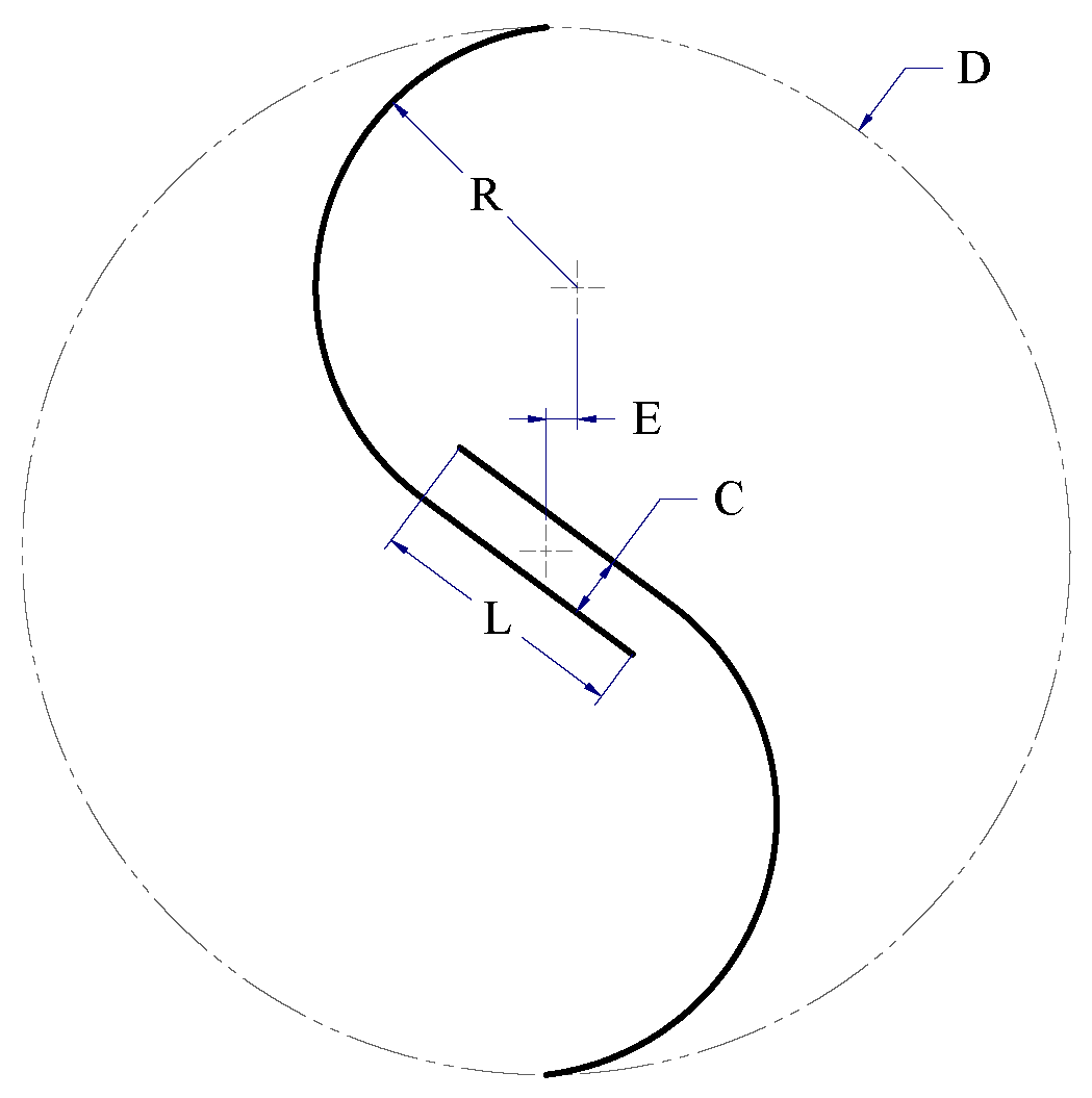
The domain analyzed consists of two parts divided by a sliding interface: a rotating circular region and a stationary rectangular region. The diameter of the circular region is 250 mm and it is located in the center of the domain. This region rotates together with the profile at a constant rate of eight revolutions per second (8 rps) corresponding to a tip speed ratio ($TSR$) of 1.2566, which is in the vicinity of the maximum performance of the profile studied. This was conducted under the assumption that the $TSR$ value corresponding to the optimal performance will not vary significantly by fixing the turbine model and the profile type. This speed was determined by simulating the rotor of dimensions corresponding to the central levels of the experimental design, rotating at different velocities so that the point of maximum performance was described.

Each simulation was carried out for ten complete revolutions of the rotor seeking to achieve a quasi-stable state. The convergence criterion for the solution residuals was set in the order of ${10}^{-3}$ for each time-step.

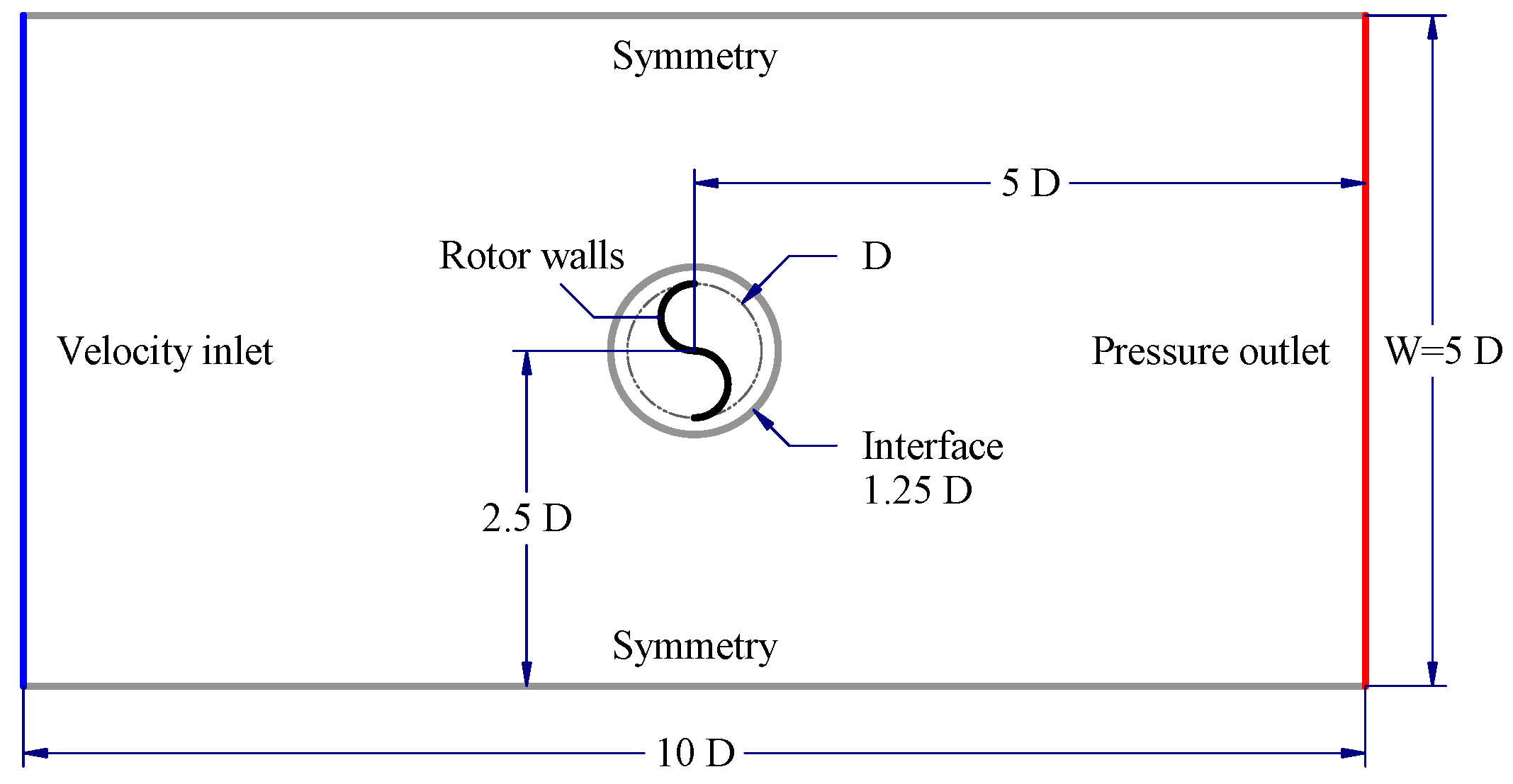
Boundary conditions were established as shown in Figure 2, using an air flow at an inlet velocity of 4 m/s (class 1 wind) [22], corresponding to a flow rate close to a number Reynolds of $6\times {10}^4$. Similarly, an output was set to atmospheric conditions and the lateral field is simulated under symmetry conditions, since there are low-scale gradients that generate negligible effects on the response variable [21]. However, the established boundary conditions can exhibit a behavior similar to a closed test section, which has less capacity to enable the flow to expand around the turbine in opposition to the restriction produced by it [23]. This makes the blockage effect caused by the rotor more significant, causing an acceleration of the flow around the obstacle and meaning an over-prediction of the rotor performance [24].

Figure 2. Analysis domain and boundary conditions.

The blockage ratio is defined as the ratio between the cross-sectional areas of the model and the test section. In a two-dimensional analysis this can be simplified as the ratio between the diameter of the rotor and the width of the flow domain ($D/W$), then the blockage effect can be also minimized by increasing the scale of the simulation domain with respect to the rotor size [24]; however, since this represents a greater requirement in computational resources, an optimal domain size is sought.

An independence analysis is performed for the computational domain, under the same conditions in which the rotor geometries were subsequently studied through the experimental design. The conventional semicircular profile is used as a test model, in order to use the result as reference when evaluating the performance of the optimized profile. The geometry is rotated at a velocity of 5 rps ($TSR=0.7854$), which is close to the maximum performance of the tested profile. This velocity is determined by simulating the rotor at different velocities, seeking to describe the optimum point.

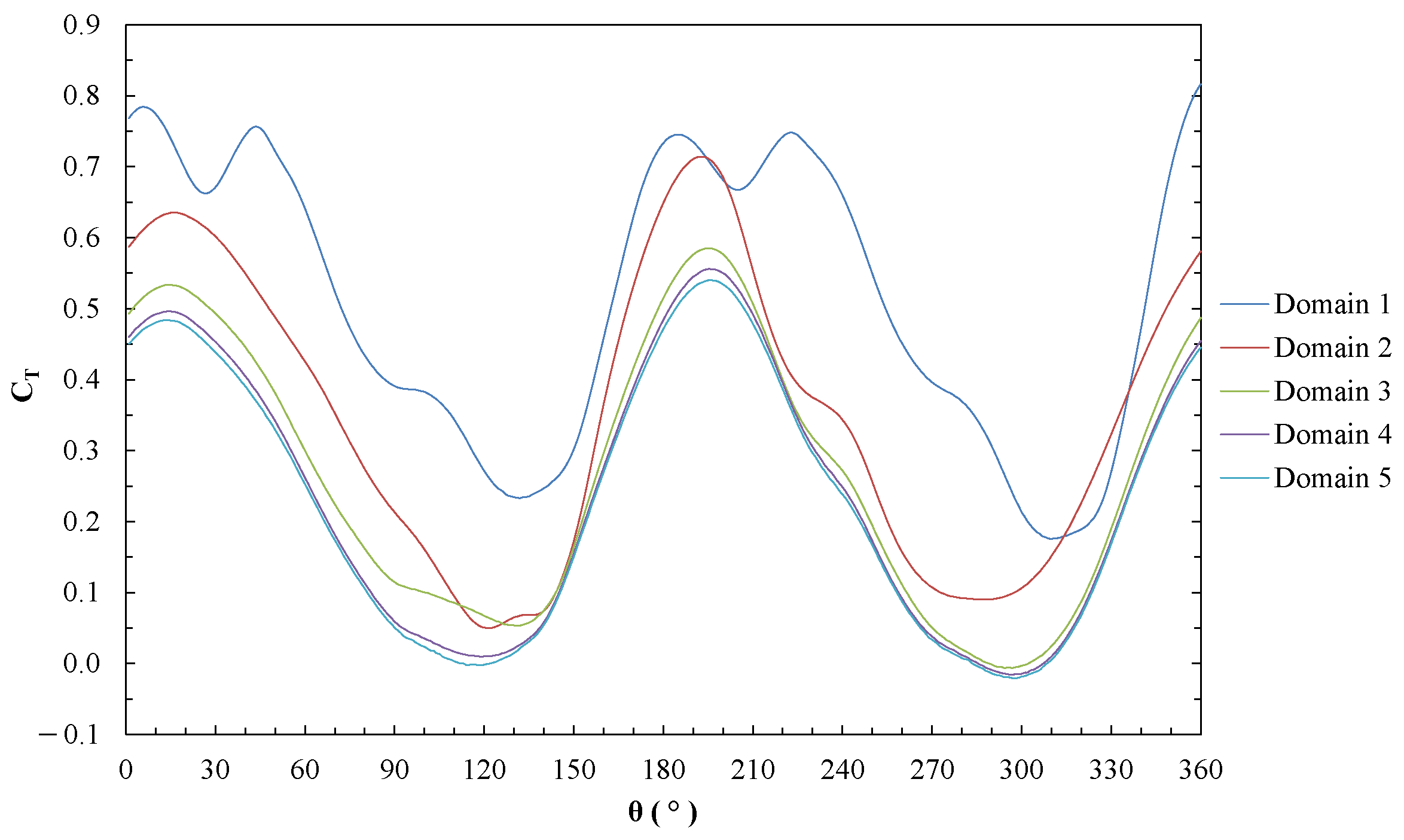
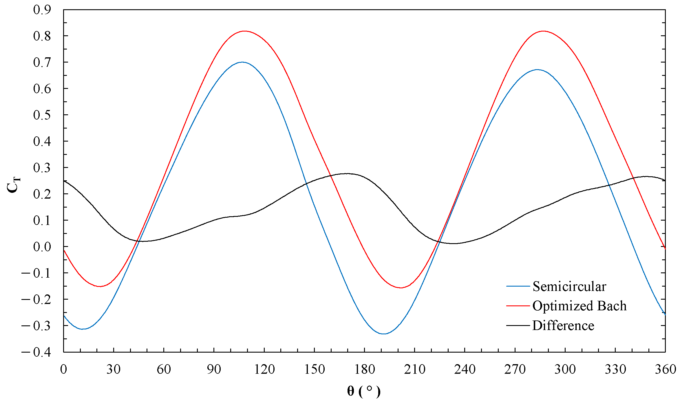
The results obtained in this analysis describe the behavior of the torque coefficient ($C_T$) according to the azimuth angle of the rotor ($\theta$) for each of the domains tested (Figure 3). $C_T$ is estimated as the ratio between the torque generated by the turbine on its axis and the torque that can be generated under the referred conditions [25,26]. This coefficient can be calculated by Equation (1), where $\rho$ is the air density, v is the wind velocity in free flow and $A=DH$ is the transverse area of the turbine, H being the height of it (unitary in two-dimensional analysis).

$$C_T=\frac{T_{turbine}}{T_{available}}=\frac{T}{\frac{1}{4}\rho A{v}^{2}D}$$

(1)

Figure 3. Torque coefficient ($C_T$) according to azimuth ($\theta$) for each domain.

When estimating the average $C_T$ for each computational domain, it is observed that its variation becomes smaller when compared to the value corresponding to the largest scale domain, indicating that there is convergence in the result. Table 2 shows the results obtained by testing the different computational domains.

Table 2. Domain independence test results.

Domain	1	2	3	4	5
Blockage ratio $(D/W)$	0.4	0.2	0.1	0.05	0.025
Number of elements	89,620	115,224	217,637	627,292	2,265,909
Averaged $C_T$	0.5091	0.3458	0.2634	0.2355	0.2274
Deviation	123.86%	52.08%	15.83%	3.58%
Simulation time [h]	4.84	6.22	11.74	33.84	122.25

It is evident that the domain size has a notable effect on the profile performance (i.e., on the averaged $C_T$). Despite this, since the same boundary conditions and domain size will be used for all the geometries studied, a significant variation within the experimental design results would not be observed. Therefore, even though different results are found, their relation with each other will be preserved [23]. The general dimensions of the domain were established according to the study carried out by [27], in which they use a domain of dimensions corresponding to the second one, with a blockage ratio of 20% (Figure 2).

Before any numerical study is conducted, an independence analysis for spatial and temporal discretizations is required, i.e., an efficient number of partitions must be obtained, in which both the analysis geometry and the period to be simulated must be divided, aiming at obtaining a convergence in the result.

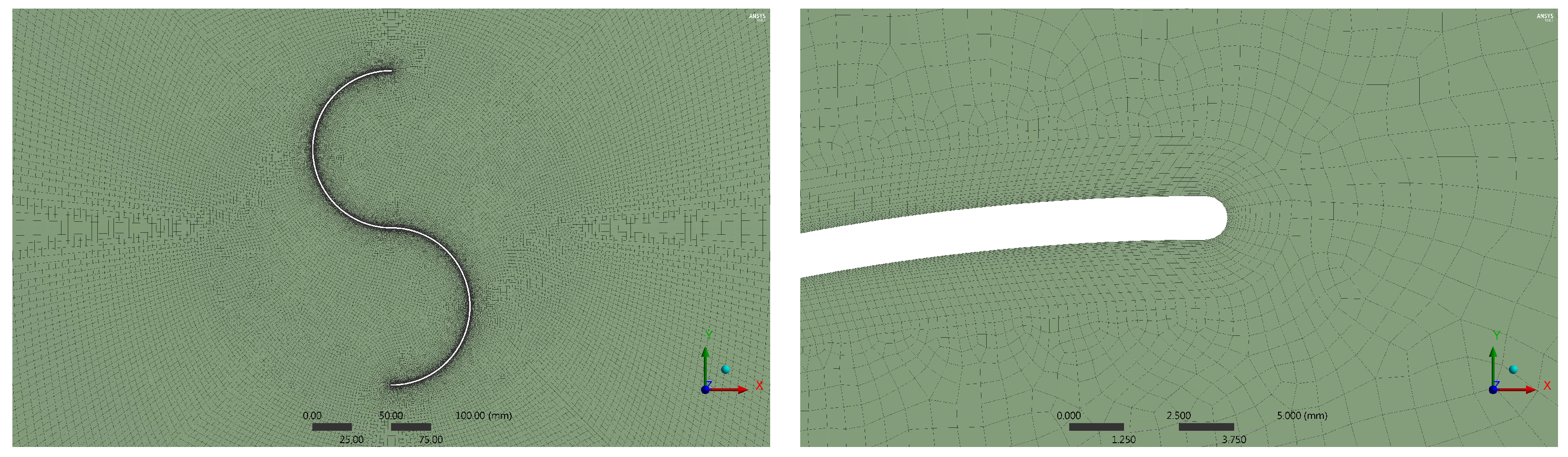
The spatial independence analysis is carried out under the same conditions and for the same geometry as the domain independence analysis. Five discretizations known as meshes are built, with the same structure but with a binomial growth in the number of partitions of each edge according to the refinement of each one. The static body that simulates the fluid in the far field has a structured mesh with only quadrilateral elements, while the mobile body that simulates the field near the rotor has an unstructured mesh with predominant quadrilateral elements and some triangular ones to achieve a greater adaptability to geometry (Figure 4 left). The meshing referring to the rotor walls is refined and has a structure by perpendicular layers (inflation) that allow a better prediction of the flow in the boundary layer conditions (Figure 4 right).

Figure 4. General structure of the mesh (left) and details of the mesh near the profile walls (right).

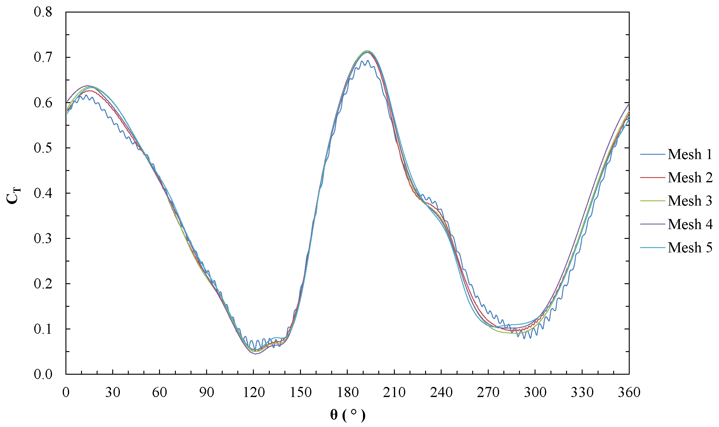
Similarly, the results obtained in this analysis describe the behavior of the $C_T$ according to $\theta$ for each mesh (Figure 5). When estimating the average $C_T$ for each mesh, its variation is observed to be is minimal when compared to the corresponding value of the finest mesh, indicating that there is convergence in the result.

Figure 5. Torque coefficient ($C_T$) according to azimuth ($\theta$) for each mesh.

A second relevant parameter for the selection of the mesh is the value of $y^{+}$, which is recommended less than unity when using the $k-\omega SST$ turbulence model, thus ensuring adequate predictions in the flow close to the walls [21]. According to the above, the fourth mesh was selected, which also requires a much shorter simulation time than the finest mesh (Table 3).

Table 3. Mesh independence test results.

Mesh	1	2	3	4	5
Number of elements	18,044	45,729	115,224	319,267	998,063
Averaged $C_T$	0.3420	0.3461	0.3458	0.3492	0.3488
Deviation	1.95%	0.77%	0.85%	0.11%
$y^{+}$	2.91	1.91	1.18	0.66	0.36
Simulation time [h]	3.67	4.43	6.22	13.87	40.10

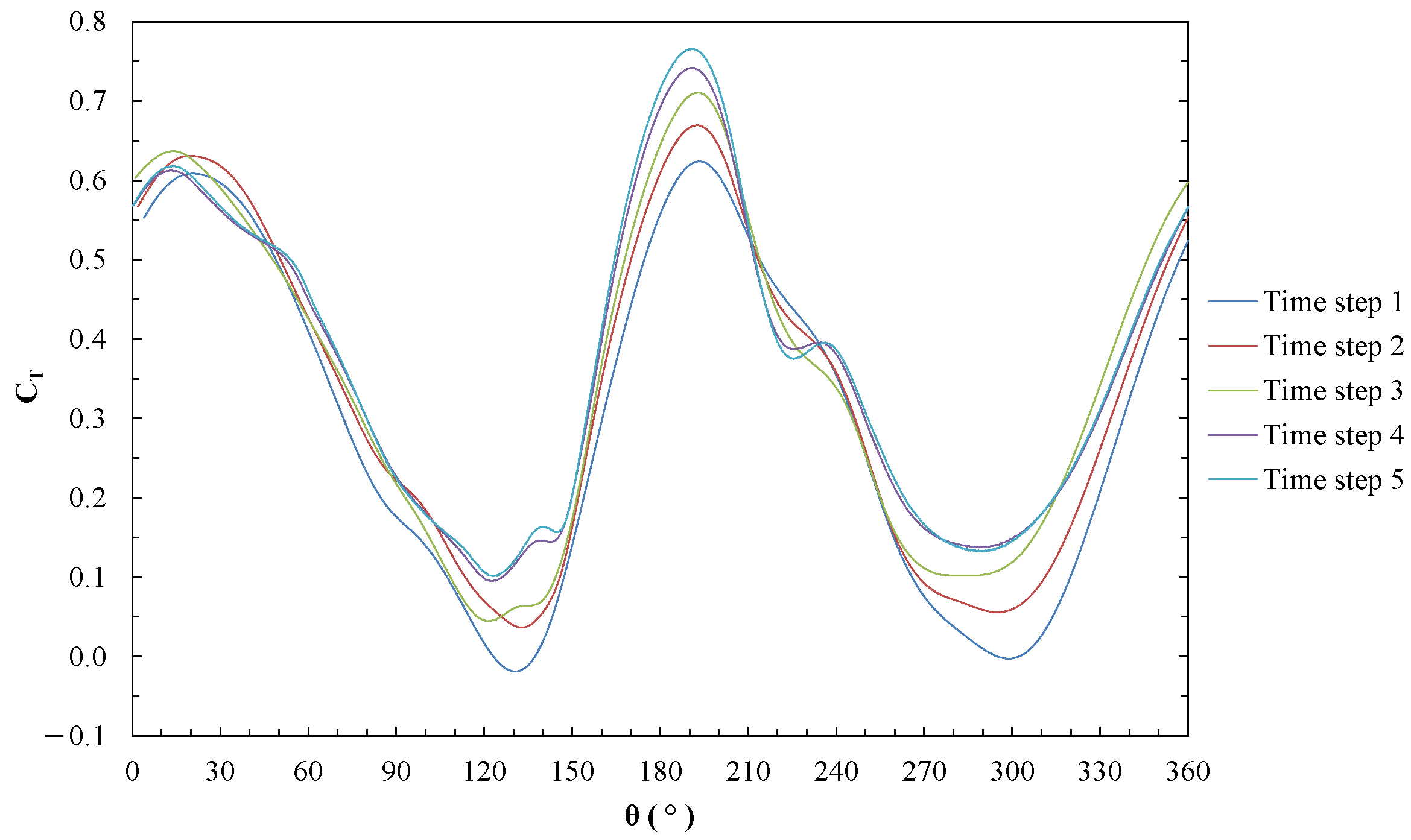
The independence analysis for temporal discretization was carried out in a similar way, under the same conditions and for the same geometry as the mesh independence analysis. Using the fourth mesh, five time discretizations were considered, generated by dividing the rotor revolution period into a number of elements or time steps. The results obtained in this analysis describe the behavior of the $C_T$ according to $\theta$ for each time steps used (Figure 6). When estimating the average value of $C_T$ for each temporal discretization, it is evident that its variation decreases as the partition becomes finer, getting closer and closer to a convergence value. A discretization of 720 time steps per revolution is determined, which represents a suitable ratio between the admissible error and the simulation time (Table 4).

Figure 6. Torque coefficient ($C_T$) according to azimuth ($\theta$) for each time step.

Table 4. Temporal independence test results.

Time Step	1	2	3	4	5
Number of elements [TS/rev]	90	180	360	720	1440
Time step size [s]	1/450	1/900	1/1800	1/3600	1/7200
Averaged $C_T$	0.2995	0.3323	0.3492	0.3649	0.3706
Deviation	19.17%	10.32%	5.77%	1.52%
Simulation time [h]	4.40	7.83	13.87	25.63	46.02

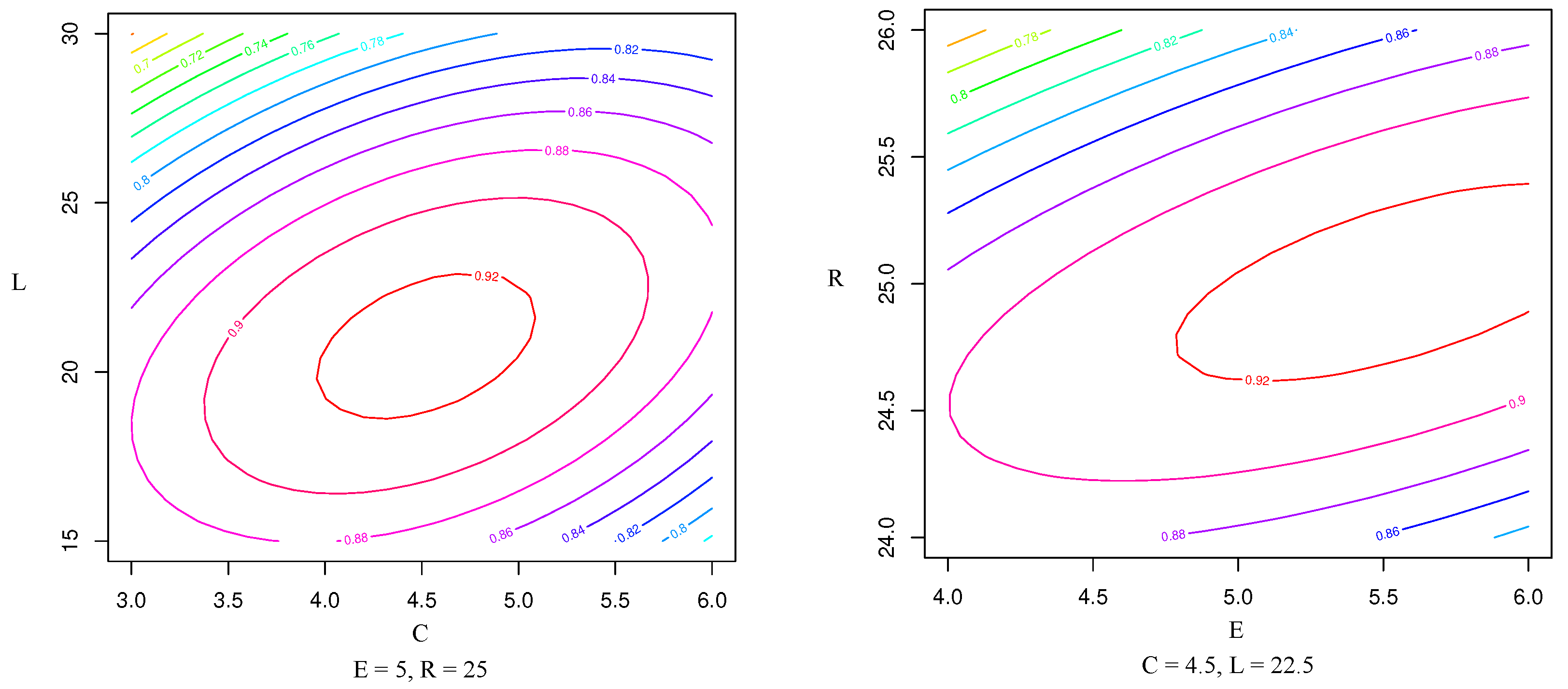
The performance of each profile is evaluated in terms of $C_T$ and the $C_P$ for the established $TSR$ value. $C_P$ consists of the ratio between the power generated by the turbine and the energy flow carried by the fluid. This can be estimated by means of Equation (2), where $\omega$ is the angular velocity of the turbine [25,26].

$$C_P=\frac{P_{turbine}}{P_{available}}=\frac{T\omega }{\frac{1}{2}\rho A{v}^3}=\frac{T}{\frac{1}{4}\rho A{v}^{2}D}\frac{\omega D}{2v}$$

(2)

Taking into consideration that the $TSR$ can be estimated according to Equation (3), Equation (2) can be rewritten as Equation (4).

$$TSR=\frac{\omega D}{2v}$$

(3)

$$C_P=C_T·TSR$$

(4)

In the numerical simulations, a reading is taken of the $C_T$ generated on the rotor axis for each angular position. These values are averaged for the last two complete revolutions, corresponding to the results of greater stability in their periodicity. This average $C_T$ allows estimating the average $C_P$ through the Equation (4). In this regard, the same process was conducted with all the geometries studied, obtaining the $C_P$ values corresponding to each combination of the experimental design.

3. Results

3.1. Hypothesis Testing

The statistical analysis required by the response surface methodology is carried out by means of R 3.6.1 programming software. The $C_P$ values obtained from the simulations are the input for the referred analysis; therefore, they must be fitted to a normal distribution to guarantee the validity of the regression model. Additionally, the residuals obtained from the regression must be non-autocorrelated, normally distributed and with a constant variance respecting each factor (i.e., Homoscedasticity must be assured). Normality distribution of the response variable and the residuals is verified with the Kolmogorov-Smirnov test and the Jarque-Bera test, respectively. Likewise, the assumptions of independence and Homoscedasticity in the residuals are verified under the Wald-Wolfowitz and Levene tests, respectively [28].

Since the calculated $C_P$ values do not fit a normal distribution, it is necessary to redistribute the data. For this, a power transformation is performed using data with a $\lambda$ exponent, so that the transformed data meet the aforementioned conditions. Several power transformations are performed with exponents between 1 and 10, and for each one a second order multiple regression model with interactions is fitted [29]. When performing the hypothesis tests for each of the regression models, their verisimilitude is evaluated, establishing a confidence interval of 95% for compliance, which corresponds to a minimum significance level of 0.05. As observed in Figure 7 left, for an exponent of 2.5, the p-values of the tests are simultaneously greater than the established level of significance; therefore, the hypothesis that leads to the requirements compliance cannot be rejected. Likewise, the expression described in Equation (5) is established to transform the data, where $C_{P}T$ is the transformed power coefficient.

$$C_{P}T=10·C_P^{2.5}$$

(5)

Figure 7. Significance level resulting from the normality and independence tests (left), and the Homoscedasticity test (right) for different power transformations (the black line represents the minimum significance level of 0.05).

Likewise, Figure 7 shows the results of the Homoscedasticity test performed on the same regression models obtained from the different power transformations. The p-values corresponding to the transformation with the exponent of 2.5, show that factors C and R probably do not present a constant variance. However, if this assumption is violated, the F test used to validate the level of significance of the factors, in balanced and deterministic models, is only slightly affected [28].

Table 5 summarizes the results of the tests performed on the fit of the regression model.

Table 5. Results of the tests in the adjustment of the regression model.

Hypothesis	Term	Test Name	p-Value	Decision
Normality	Response variable ($C_{P}T$)	Kolmogorov-Smirnov	0.05586	Cannot be rejected
Normality	Residuals	Jarque-Bera	0.9965	Cannot be rejected
Independence	Residuals	Wald-Wolfowitz (runs test)	0.0658	Cannot be rejected
Homoscedasticity	C: Gap	Levene	0.0001701	Can be rejected
Homoscedasticity	L: Overlap	Levene	0.4887	Cannot be rejected
Homoscedasticity	E: Eccentricity	Levene	0.06262	Cannot be rejected
Homoscedasticity	R: Blade radius	Levene	3.418 $\times {10}^{-8}$	Can be rejected

3.2. Response Surface

The results of the numerical simulations for each FFD treatment are shown in order according to their factors in Table 6.

Table 6. Power coefficient ($C_P$) determined for each treatment of the FFD.

C	L	E	R	${\mathit{C}}_{\mathit{P}}$	C	L	E	R	${\mathit{C}}_{\mathit{P}}$	C	L	E	R	${\mathit{C}}_{\mathit{P}}$	C	L	E	R	${\mathit{C}}_{\mathit{P}}$
3	15	4	24	0.3755	3	20	6	24	0.3754	3	25	5	25	0.3716	3	30	4	26	0.2810
4	15	4	24	0.3601	4	20	6	24	0.3608	4	25	5	25	0.3881	4	30	4	26	0.2939
5	15	4	24	0.3465	5	20	6	24	0.3517	5	25	5	25	0.3875	5	30	4	26	0.3044
6	15	4	24	0.3375	6	20	6	24	0.3294	6	25	5	25	0.3819	6	30	4	26	0.3152
3	20	4	24	0.3843	3	25	6	24	0.3845	3	30	5	25	0.3193	3	15	5	26	0.3373
4	20	4	24	0.3769	4	25	6	24	0.3762	4	30	5	25	0.3484	4	15	5	26	0.3855
5	20	4	24	0.3600	5	25	6	24	0.3635	5	30	5	25	0.3651	5	15	5	26	0.3828
6	20	4	24	0.3498	6	25	6	24	0.3417	6	30	5	25	0.3729	6	15	5	26	0.3722
3	25	4	24	0.3824	3	30	6	24	0.3736	3	15	6	25	0.3781	3	20	5	26	0.3341
4	25	4	24	0.3846	4	30	6	24	0.3864	4	15	6	25	0.3684	4	20	5	26	0.3742
5	25	4	24	0.3767	5	30	6	24	0.3525	5	15	6	25	0.3577	5	20	5	26	0.3910
6	25	4	24	0.3694	6	30	6	24	0.3379	6	15	6	25	0.3428	6	20	5	26	0.3840
3	30	4	24	0.3372	3	15	4	25	0.3845	3	20	6	25	0.3886	3	25	5	26	0.3220
4	30	4	24	0.3587	4	15	4	25	0.3783	4	20	6	25	0.3808	4	25	5	26	0.3536
5	30	4	24	0.3561	5	15	4	25	0.3648	5	20	6	25	0.3665	5	25	5	26	0.3722
6	30	4	24	0.3482	6	15	4	25	0.3568	6	20	6	25	0.3586	6	25	5	26	0.3827
3	15	5	24	0.3704	3	20	4	25	0.3877	3	25	6	25	0.3736	3	30	5	26	0.3008
4	15	5	24	0.3573	4	20	4	25	0.3876	4	25	6	25	0.3880	4	30	5	26	0.3187
5	15	5	24	0.3414	5	20	4	25	0.3793	5	25	6	25	0.3810	5	30	5	26	0.3323
6	15	5	24	0.3294	6	20	4	25	0.3717	6	25	6	25	0.3744	6	30	5	26	0.3423
3	20	5	24	0.3801	3	25	4	25	0.3372	3	30	6	25	0.3220	3	15	6	26	0.3436
4	20	5	24	0.3710	4	25	4	25	0.3852	4	30	6	25	0.3614	4	15	6	26	0.3838
5	20	5	24	0.3600	5	25	4	25	0.3901	5	30	6	25	0.3747	5	15	6	26	0.3756
6	20	5	24	0.3467	6	25	4	25	0.3865	6	30	6	25	0.3810	6	15	6	26	0.3619
3	25	5	24	0.3849	3	30	4	25	0.3108	3	15	4	26	0.3308	3	20	6	26	0.3395
4	25	5	24	0.3808	4	30	4	25	0.3475	4	15	4	26	0.3682	4	20	6	26	0.3917
5	25	5	24	0.3682	5	30	4	25	0.3571	5	15	4	26	0.3859	5	20	6	26	0.3854
6	25	5	24	0.3580	6	30	4	25	0.3503	6	15	4	26	0.3778	6	20	6	26	0.3772
3	30	5	24	0.3451	3	15	5	25	0.3815	3	20	4	26	0.3159	3	25	6	26	0.3260
4	30	5	24	0.3580	4	15	5	25	0.3733	4	20	4	26	0.3452	4	25	6	26	0.3666
5	30	5	24	0.3590	5	15	5	25	0.3605	5	20	4	26	0.3735	5	25	6	26	0.3879
6	30	5	24	0.3646	6	15	5	25	0.3471	6	20	4	26	0.3886	6	25	6	26	0.3861
3	15	6	24	0.3626	3	20	5	25	0.3910	3	25	4	26	0.2904	3	30	6	26	0.3039
4	15	6	24	0.3521	4	20	5	25	0.3843	4	25	4	26	0.3028	4	30	6	26	0.3306
5	15	6	24	0.3373	5	20	5	25	0.3732	5	25	4	26	0.3196	5	30	6	26	0.3496
6	15	6	24	0.3236	6	20	5	25	0.3664	6	25	4	26	0.3260	6	30	6	26	0.3744

The results of the global Fisher F test allow concluding with a full confidence that the analyzed data respond to a trend and, therefore, can be modeled (p-value < 2.2 $\times {10}^{-16}$). The second order multiple regression model with interactions is adjusted, which the effect of the factors studied is determined with. The null hypothesis of the test establishes that the analyzed factor has no effect on the response variable. Therefore, the p-value is sought to be less than the established significance level of 0.05, to conclude reciprocally with a minimum confidence level of 95%. Likewise, the lower the p-value of each coefficient, the greater the evidence against the null hypothesis, which suggests a significant difference generated by the respective factor [30]. Table 7 summarizes the results of the analysis of variance (ANOVA) for the fitted regression model.

Table 7. ANOVA for the regression model adjusted. (DOF), (SS), and (MS) refers to degrees of freedom, sum of squares, and mean squares, respectively.

Term	DOF	SS	MS	t-Value	p-Value
FO (C, L, E, R)	4	0.25905	0.064762	17.639	1.43 $\times {10}^{-11}$
TWI (C, L, E, R)	6	1.13904	0.189839	51.706	<2.20 $\times {10}^{-16}$
PQ (C, L, E, R)	4	0.49255	0.123137	33.538	<2.20 $\times {10}^{-16}$
Residuals	129	0.47363	0.003672
Lack of fit	129	0.47363	0.003672
Pure error	0	0

Table 8 shows the results of the statistic tests for each factor.

Table 8. Results of the test statistics for each factor.

Term	Coefficient	Std. Error	t-Value	p-Value
Intercept	−35.89	6.8223	−5.2606	5.80 $\times {10}^{-7}$
C: Gap	−1.429	0.14934	−9.5687	<2.20 $\times {10}^{-16}$
L: Overlap	0.2607	0.029869	8.7282	1.14 $\times {10}^{-14}$
E: Eccentricity	−0.96413	0.22047	−4.3731	2.50 $\times {10}^{-5}$
R: Blade radius	3.1832	0.5381	5.9156	2.80 $\times {10}^{-8}$
$C:L$	0.0050934	0.00080791	6.3044	4.23 $\times {10}^{-9}$
$C:E$	−0.010143	0.0055314	−1.8338	0.06899
$C:R$	0.063614	0.0055314	11.5006	<2.20 $\times {10}^{-16}$
$L:E$	0.0055328	0.0011063	5.0013	1.82 $\times {10}^{-6}$
$L:R$	−0.0097194	0.0011063	−8.7857	8.26 $\times {10}^{-15}$
$E:R$	0.043286	0.0075742	5.7149	7.23 $\times {10}^{-8}$
$C^2$	−0.023919	0.0050494	−4.737	5.63 $\times {10}^{-6}$
$L^2$	−0.001647	0.00020198	−8.1546	2.68 $\times {10}^{-13}$
$E^2$	−0.017731	0.010711	−1.6553	0.10029
$R^2$	−0.06981	0.010711	−6.5173	1.47 $\times {10}^{-9}$

Factors C and L have the lowest p-values among the main effects, indicating that there is more evidence of having the greatest effect on the response variable. In the same way it happens with the interactions C:L, C:R and L:R, whose p-value close to 0, demonstrates the great dependence that exists between each pair of factors, in addition to their significance within the model. This result confirms the importance of analyzing the factors together in order to consider the variation of each one, with respect to the variation of a second factor. The quadratic effects of the L and R factors are also highly significant, indicating that their trend presents a curvature that must be taken into account in the fitted model and, therefore, validates the implementation of the second order model.

The quadratic effect of the factor E and the interaction C:E exceeds the minimum significance level of 0.05. However, its value is close to 0.10, which allows a conclusion with 90% confidence. For this reason they are kept within the model.

The coefficients corresponding to each factor constitute the regression polynomial that determines the value of the response variable transformed in each of the coordinates [31]. The referred regression polynomial is expressed in Equation (6), whose goodness of fit is defined by a $R^2$ of 0.7997 and an adjusted $R^2$ of 0.7779.

$$\begin{array}{cc}\hfill C_{P}T& =-35.89-1.429·C+0.2607·L-0.96413·E+3.1832·R\hfill \\ \hfill & +0.0050934·CL-0.010143·CE+0.063614·CR+0.0055328·LE-0.0097194·LR\hfill \\ \hfill & +0.043286·ER-0.023919·C^2-0.001647·L^2-0.017731·E^2-0.06981·R^2\hfill \end{array}$$

(6)

Figure 8 shows the surface graphs obtained by evaluating the regression polynomial in the central values of two factors and as a function of the remaining two factors.

Figure 8. Response surfaces perspective graphs.

To determine the geometric proportions resulting in the maximum performance of the rotor, finding the point at which the value of the derivative of the regression polynomial becomes zero is needed. Figure 9 allows obtaining a better appreciation of the stationary points of the surfaces illustrated in Figure 8.

Figure 9. Response surfaces contour graphs.

The coordinates of the global stationary point, at which all the model factors have a zero slope simultaneously, are shown in Equation (7).

$$(C,L,E,R)=(4.69,21.45,5.52,25.15)$$

(7)

By constructing the profile with the optimal proportions and simulating it under the same conditions as the previous geometries, a $C_P$ of 0.3922 is obtained, which resulted to be higher than all the performance values obtained in the experimental design. On the other hand, replacing these coordinates in the regression polynomial results in a $C_{P}T$ of 0.9293, corresponding to a $C_P$ of 0.3866. This means an error of 1.4278%, between the performance obtained numerically and that estimated using the regression model, as shown in Equation (8).

$$E_r=\frac{0.3922-0.3866}{0.3922}\times 100\%=1.4278\%$$

(8)

3.3. Performance Analysis of the Optimized Profile

The discretization independence analysis was carried out using the conventional semicircular profile with the purpose of serving as a reference. This one presented a $C_T$ of 0.3649 at a $TSR$ of 0.7854, thus, according to Equation (4), a $C_P$ of 0.2866 was obtained. In contrast, the optimized Bach profile allowed reaching a $C_P$ of 0.3922, which is 36.8% higher. To understand the aspects that led to this result, the behavior of the aerodynamic coefficients of each rotor is analyzed as a function of its azimuthal position.

The position in which the greatest performance difference is presented, between both blade profiles, corresponds to the alignment that supposes greater opposition to flow, that is, at angles close to 0° and 180° (Figure 10). Additionally, as observed in Table 9, the average value of the drag coefficient ($C_x$) increased, while the lift coefficient ($C_y$) decreased, indicating that the advantage of the optimized profile over the reference profile is mainly due to the optimization of the drag force.

Figure 10. Difference between the torque coefficient ($C_T$) of the conventional semicircular profile and the optimized Bach, at a $TSR$ of 1.0996.

Table 9. Average, drag, lift and resulting coefficients on the rotor.

	Semicircular	Optimized Bach	Difference
$C_x$	1.2786	1.4927	16.74%
$C_y$	1.5878	1.5558	−2.02%
$C_{total}$	2.0386	2.1560	5.76%

In the contour graphs, the pressure and flow velocity states are shown through the studied geometries. These are aligned in the position where the greatest difference in the performance between the two rotors is appreciated. It is evident that the pressure on the concave side of the advancing blade is higher for the optimized profile (Figure 11 left) than for the reference profile (Figure 11 right). This is due to the fact that the existing flow through the opening generated by the division of the profile (Figure 12 left) avoids the early depressurization of the referred region, and consequently increases the moment produced in the rotor axis, in addition to enabling to get a higher turning velocity [32]. Similarly, it can be found that in the semicircular profile there is a region of higher velocity in the concavity of the returning blade (Figure 12 right), which is caused by the vorticity that is generated in this area. This higher velocity induces a lower pressure and also generates a greater resistance to blade movement.

Figure 11. Pressure contour graphs for the optimized Bach profile (left) and the conventional semicircular profile (right) at a $TSR$ of 1.0996.

Figure 12. Velocity contour graphs for the optimized Bach profile (left) and the conventional semicircular profile (right) at a $TSR$ of 1.0996.

4. Discussion

The FFD involves a higher number of treatments compared to other experimental designs, meaning that a greater number of resources is required. Seeking to carry out a comparative analysis that allows assessing the referred experimental design; a FCCD is performed under a procedure similar to that previously detailed for the FFD. For this, the data matrix is complemented, calculating the values corresponding to the central treatments. The results of the numerical simulations for each treatment of the FCCD are ordered shown according to their factors in Table 10.

Table 10. Power coefficient ($C_P$) determined for each treatment of the FCCD.

C	L	E	R	${\mathit{C}}_{\mathit{P}}$	C	L	E	R	${\mathit{C}}_{\mathit{P}}$	C	L	E	R	${\mathit{C}}_{\mathit{P}}$
3	15	4	24	0.3755	4.5	15	4	25	0.3716	3	15	4	26	0.3308
6	15	4	24	0.3375	3	22.5	4	25	0.3660	6	15	4	26	0.3778
4.5	22.5	4	24	0.3759	4.5	22.5	4	25	0.3900	4.5	22.5	4	26	0.3340
3	30	4	24	0.3372	6	22.5	4	25	0.3822	3	30	4	26	0.2810
6	30	4	24	0.3482	4.5	30	4	25	0.3550	6	30	4	26	0.3152
4.5	15	5	24	0.3492	3	15	5	25	0.3815	4.5	15	5	26	0.3868
3	22.5	5	24	0.3847	6	15	5	25	0.3471	3	22.5	5	26	0.3291
4.5	22.5	5	24	0.3718	4.5	22.5	5	25	0.3853	4.5	22.5	5	26	0.3771
6	22.5	5	24	0.3531	3	30	5	25	0.3193	6	22.5	5	26	0.3865
4.5	30	5	24	0.3582	6	30	5	25	0.3729	4.5	30	5	26	0.3260
3	15	6	24	0.3626	4.5	15	6	25	0.3634	3	15	6	26	0.3436
6	15	6	24	0.3236	3	22.5	6	25	0.3850	6	15	6	26	0.3619
4.5	22.5	6	24	0.3644	4.5	22.5	6	25	0.3807	4.5	22.5	6	26	0.3883
3	30	6	24	0.3736	6	22.5	6	25	0.3668	3	30	6	26	0.3039
6	30	6	24	0.3379	4.5	30	6	25	0.3701	6	30	6	26	0.3744

These results conform to a normal distribution and meet with the aforementioned statistical requirements without requiring a power transformation. Fitting the second order multiple regression model with interactions, the results shown in Table 11 are obtained.

Table 11. Comparative between the FFD and FCCD designs.

	Number of	${\mathit{R}}^2$	Adjusted	Modeled	Numerical	Stationary Point
	Treatments		${\mathit{R}}^2$	${\mathit{C}}_{\mathit{P}}$	${\mathit{C}}_{\mathit{P}}$	C	L	E	E
FFD	144	0.7997	0.7779	0.3866	0.3922	4.6906	21.4484	5.5213	25.1545
FCCD	45	0.8603	0.7951	0.3878	0.3788	5.1711	22.7178	6.3175	25.4853
Difference	−68.75%	7.58%	2.21%	0.30%	−3.42%	10.24%	5.92%	14.42%	1.32%

Table 11 shows a significant decrease in the number of treatments required by the FCCD with respect to the FFD, leading to a reduction in the involved resources of almost 70%. Additionally, the $C_P$ estimated through these models largely preserves their order of magnitude.

However, the optimal points estimated using the regression models for each of the designs show significant differences, mainly in C and E factors. Likewise, by simulating the geometries built from these optimal parameters, the FFD presents a more favorable performance result, which leads to a greater acceptance of this model for the purposes of this research. On the other hand, although the goodness of fit seems significantly higher for the FCCD with a difference of 7.58% in the value of $R^2$, the adjusted $R^2$ is only 2.21% higher, which reveals a greater effect of the factors on the response variable in the FFD rather than in the FCCD. This can be verified in Figure 13, where a supremacy in the scale of the effects of each of the factors and their interactions is identified, indicating that it is possible to capture more information from the data in the first design than in the second one. This may be the root cause of optimal point prediction in the FFD being more accurate.

Figure 13. Significance level for the different factors and interactions in the FFD and FCCD designs (the black line represents the maximum significance level of 0.05).

To verify the numerical results, the experimental results reported in the study developed by Gallo et al. [33] are considered (Figure 14). The experiments were carried out in a wind tunnel with a closed test section of 50 cm × 50 cm and a rotor model of 200 mm in diameter and 200 mm height, corresponding to a blockage ratio of 16%. Three profile configurations are tested including the conventional semicircular and the split Bach, at a velocity of 4 m/s, corresponding to a Reynolds number of $6\times {10}^4$ used in this study. The dimensions of the Bach profile used in the study correspond to the values of the parameters C, L, E and R of 4.69, 21.45, 5.52 and 25.15, respectively.

Figure 14. Performance graph for the semicircular and Bach profiles for the blockage uncorrected condition.

Figure 14 shows that the $TSR$ value assumed in the development of the study as the condition of maximum performance for the two types of profile is largely adjusted for the established conditions.

With the purpose of obtaining a better estimate of the real turbine performance, the optimized rotor simulation is carried out using a larger scale simulation domain. A square domain whose side is 50 times the diameter of the rotor is used, seeking to minimize the blockage effect produced by the rotor in the flow field. Conventional semicircular geometry is also analyzed under the same conditions, with blockage ratio of 2%.

Additionally, to verify the numerical results with blockage corrected, the experimental results reported in the study developed by Roy and Saha [12] are considered. The experiments were carried out in a wind tunnel at a velocity range of 0–10 m/s, comprising the flow corresponding to a Reynolds number of $6\times {10}^4$. Different profile configurations are tested including the split semicircular and the split Bach, with a rotor diameter of 209 mm and a height of 230 mm. The dimensions of the Bach profile used in the study correspond to the values of the parameters C, L, E and R of 5.40, 23.08, 6.22 and 25.01, respectively. The results described above are related in Figure 15.

Figure 15. Performance graph for the semicircular and Bach profiles for the blockage corrected condition.

Figure 14 and Figure 15 show that the results obtained from the numerical study, are adjusted to the order of magnitude of the experimental data for the two types of profile [12,33]. The main difference occurs in the rate of rotation in which the Bach type profile reaches its maximum performance, which may be due to the fact that the inertia of the system is not considered in the numerical analysis, in addition to the other causes of error specific to each of the approaches.

On the other hand, the superior performance of the optimized Bach profile respecting the semicircular profile can be evidenced, and how this predominance is preserved regardless of the blockage condition or the approach (numerical or experimental). In Table 12 it can be observed that the increase in the performance between the two profiles maintains its order of magnitude for both blockage conditions. Similarly, the deviation between the simulation results without correction and with blockage correction is significantly the same for both profiles, indicating that the domain size is not a relevant variation factor within the experimental design.

Table 12. Performance of the semicircular profile and optimized Bach profile according to their blockage condition.

	Averaged ${\mathit{C}}_{\mathit{P}}$		Deviation
	Blockage Uncorrected	Blockage Corrected
Semicircular	0.2866	0.1950	47.00%
Optimized Bach	0.3922	0.2661	47.35%
Increase	36.83%	36.50%

5. Conclusions

In the present investigation, the optimal proportions of a Savonius rotor with a split Bach blade profile without intermediate shaft have been determined numerically. The results showed that all the factors analyzed had statistically significant effects on the $C_P$ in the studied experimental domain. The dimensions of the overlap corresponding to factors C and L proved to be the most relevant. The dimensions of the blade curvature defined by the factors E and R presented lower effects individually, however they showed very significant interactions with the other factors. In summary, it was observed that there is a great interaction between the evaluated factors, which validates the importance of the new methodology used. The optimal dimensions obtained for referred profile are 4.69, 21.45, 5.52 and 25.15 in percentage values of the rotor diameter, for parameters C, L, E and R parameters, respectively.

Although the FFD was more accepted for the purposes of this research, the FCCD also enables the rotor performance to be modeled with a great precision, requiring only 31.25% of treatments.

The conventional semicircular profile established as reference, presented a $C_P$ of 0.195 in a flow close to a Reynolds number of $6\times {10}^4$ and a blockage ratio of 2%. In turn, the geometry with the blade profile optimized by the response surface methodology presented a $C_P$ of 0.2661, under the same conditions, representing a 36.5% increase in the performance respect to the reference profile.

References

- Savonius, S.J. The S-rotor and its applications. Mech. Eng. 1931, 53, 333–338. [Google Scholar]
- Mohammed, A.A.; Ouakad, H.M.; Sahin, A.Z.; Bahaidarah, H. Vertical axis wind turbine aerodynamics: Summary and review of momentum models. J. Energy Resour. Technol. 2019, 141, 5. [Google Scholar] [CrossRef]
- Eriksson, S.; Bernhoff, H.; Leijon, M. Evaluation of different turbine concepts for wind power. Renew. Sustain. Energy Rev. 2008, 12, 1419–1434. [Google Scholar] [CrossRef]
- Chen, L.; Chen, J.; Zhang, Z. Review of the Savonius rotor’s blade profile and its performance. J. Renew. Sustain. Energy 2018, 10, 013306. [Google Scholar] [CrossRef]
- Golecha, K.; Kamoji, M.; Kedare, S.; Prabhu, S. Review on Savonius rotor for harnessing wind energy. Wind. Eng. 2012, 36, 605–645. [Google Scholar] [CrossRef]
- Kumar, A.; Saini, R. Performance parameters of Savonius type hydrokinetic turbine-A Review. Renew. Sustain. Energy Rev. 2016, 64, 289–310. [Google Scholar] [CrossRef]
- Bhutta, M.M.A.; Hayat, N.; Farooq, A.U.; Ali, Z.; Jamil, S.R.; Hussain, Z. Vertical axis wind turbine—A review of various configurations and design techniques. Renew. Sustain. Energy Rev. 2012, 16, 1926–1939. [Google Scholar] [CrossRef]
- Roy, S.; Saha, U.K. Review of experimental investigations into the design, performance and optimization of the Savonius rotor. Proc. Inst. Mech. Eng. Part A J. Power Energy 2013, 227, 528–542. [Google Scholar] [CrossRef]
- Savonius, S.J. Vertical Axis Wind Turbine. U.S. Patent 1,697,574, 1 January 1929. [Google Scholar]
- Bach, G.V. Untersuchungen über Savonius-rotoren und verwandte strömungsmaschinen. Forschung auf dem Gebiet des Ingenieurwesens A 1931, 2, 218–231. [Google Scholar] [CrossRef]
- Alom, N.; Saha, U.K. Influence of blade profiles on Savonius rotor performance: Numerical simulation and experimental validation. Energy Convers. Manag. 2019, 186, 267–277. [Google Scholar] [CrossRef]
- Roy, S.; Saha, U.K. Wind tunnel experiments of a newly developed two-bladed Savonius-style wind turbine. Appl. Energy 2015, 137, 117–125. [Google Scholar] [CrossRef]
- Kacprzak, K.; Liskiewicz, G.; Sobczak, K. Numerical investigation of conventional and modified Savonius wind turbines. Renew. Energy 2013, 60, 578–585. [Google Scholar] [CrossRef]
- Modi, V.; Fernando, M. On the performance of the Savonius wind turbine. J. Sol. Energy Eng. 1989, 111, 71–81. [Google Scholar] [CrossRef]
- Ismail, I.; Pane, E.; Haryanto, G.; Okviyanto, T.; Rahman, R. A better approach for modified bachtype savonius turbine optimization. Int. Rev. Aerosp. Eng. 2021, 14, 159–165. [Google Scholar]
- Ramar, S.K.; Seralathan, S.; Hariram, V. Numerical analysis of different blade shapes of a Savonius style vertical axis wind turbine. Int. J. Renew. Energy Res. (IJRER) 2018, 8, 1657–1666. [Google Scholar]
- Kamoji, M.; Kedare, S.B.; Prabhu, S. Experimental investigations on single stage modified Savonius rotor. Appl. Energy 2009, 86, 1064–1073. [Google Scholar] [CrossRef]
- Djanali, V.S.; Fathurrahman, Z.; Dwiyantoro, B.A.; Ikhwan, N. Numerical study of savonius wind turbines with standard and Bach-profile blade variations. AIP Conf. Proc. 2019, 2187, 020041. [Google Scholar]
- Gallo Jaramillo, L.A.; Chica Arrieta, E.L.; Flórez Serrano, E.G. Estudio de desempeño de distintos perfiles de álabe de una turbina eólica para aprovechar vientos de baja velocidad. Ingeniería 2022, 27, 1. [Google Scholar] [CrossRef]
- Abraham, J.; Mowry, G.; Plourde, B.; Sparrow, E.; Minkowycz, W. Numerical simulation of fluid flow around a vertical-axis turbine. J. Renew. Sustain. Energy 2011, 3, 033109. [Google Scholar] [CrossRef]
- Andersson, B.; Andersson, R.; Haakansson, L.; Mortensen, M.; Sudiyo, R.; Van Wachem, B. Computational Fluid Dynamics for Engineers; Cambridge University Press: Cambridge, UK, 2011. [Google Scholar]
- Jain, P. Wind Energy Engineering; McGraw Hill: New York, NY, USA, 2011. [Google Scholar]
- Ross, I.; Altman, A. Wind tunnel blockage corrections: Review and application to Savonius vertical-axis wind turbines. J. Wind. Eng. Ind. Aerodyn. 2011, 99, 523–538. [Google Scholar] [CrossRef]
- Roy, S.; Saha, U.K. An adapted blockage factor correlation approach in wind tunnel experiments of a Savonius-style wind turbine. Energy Convers. Manag. 2014, 86, 418–427. [Google Scholar] [CrossRef]
- Mathew, S. Wind Energy: Fundamentals, Resource Analysis and Economics; Springer: Berlin/Heidelberg, Germany, 2006. [Google Scholar] [CrossRef]
- Al-Ghriybah, M.; Zulkafli, M.F.; Didane, D.H.; Mohd, S. The effect of inner blade position on the performance of the Savonius rotor. Sustain. Energy Technol. Assess. 2019, 36, 100534. [Google Scholar] [CrossRef]
- Alom, N.; Saha, U.K. Arriving at the optimum overlap ratio for an elliptical-bladed Savonius rotor. In Turbo Expo: Power for Land, Sea, and Air; American Society of Mechanical Engineers: New York, NY, USA, 2017; Volume 50961, p. V009T49A012. [Google Scholar] [CrossRef]
- Montgomery, D.C. Design and Analysis of Experiments; John Wiley & Sons: Hoboken, NJ, USA, 2017. [Google Scholar]
- Montgomery, D.C.; Peck, E.A.; Vining, G.G. Introduction to Linear Regression Analysis; John Wiley & Sons: Hoboken, NJ, USA, 2021. [Google Scholar]
- Mason, R.L.; Gunst, R.F.; Hess, J.L. Statistical Design and Analysis of Experiments: With Applications to Engineering and Science; John Wiley & Sons: Hoboken, NJ, USA, 2003; Volume 474. [Google Scholar]
- Myers, R.H.; Montgomery, D.C.; Anderson-Cook, C.M. Response Surface Methodology: Process and Product Optimization Using Designed Experiments; John Wiley & Sons: Hoboken, NJ, USA, 2016. [Google Scholar]
- Salleh, M.B.; Kamaruddin, N.M.; Mohamed-Kassim, Z. Savonius hydrokinetic turbines for a sustainable river-based energy extraction: A review of the technology and potential applications in Malaysia. Sustain. Energy Technol. Assess. 2019, 36, 100554. [Google Scholar] [CrossRef]
- Gallo, L.A.; Chica, E.L.; Flórez, E.G.; Obando, F.A. Numerical and Experimental Study of the Blade Profile of a Savonius Type Rotor Implementing a Multi-Blade Geometry. Appl. Sci. 2021, 11, 10580. [Google Scholar] [CrossRef]
Publisher’s Note: MDPI stays neutral with regard to jurisdictional claims in published maps and institutional affiliations. |
© 2022 by the authors. Licensee MDPI, Basel, Switzerland. This article is an open access article distributed under the terms and conditions of the Creative Commons Attribution (CC BY) license (https://creativecommons.org/licenses/by/4.0/).