Abstract
Agro-management zones recently became the backbone of modern agriculture. Delineating management zones for Variable-Rate Fertilization (VRF) can provide important ecological benefits and better sustainability of the new Egyptian farming projects. This article aims to represent an approach for delineating management zones using Spatial Multicriteria Evaluation (SMCE) within irrigated peanut pivot situated at the eastern Nile Delta, Egypt. The results indicated that soil data, such as soil texture, soil type, the elevation of the landscape, and slope, allow for sampling the study area into similar classes and in smaller units, along with a crop productivity map. The effects of the variability in soil characteristics within the field on Peanut yields are predicted by the soil suitability model. In addition, final management zones map a varied amount of nutrients that could be added to different pivot zones. In conclusion, mapping soil units with a sufficient number of field observations within each class provided an acceptable accuracy, and a good spatial distribution of the suitability classification was achieved. Hence, agro-management zones are essentially needed for policymakers in a specific field in order to furnish an evaluation about the transformations at a territorial scale and for studying the strategies to realize environmental sustainability and to reduce the territorial impacts.
1. Introduction
Recently, a wide range of technologies have been utilized to make modern agriculture more efficient [1]. The rapid evolution of precision farming or site-specific management has been made possible by using the Global Positioning System (GPS) with Geographic Information Systems (GIS) techniques and remote sensing data. These data make farmers able to understand the site-specific needs of their fields [2]. Farm management practices affect the quality of soil and productivity of crops on various spatio-temporal scales [3]. Hence, the evaluation of the spatial differences in soil properties and characteristics is very important for field management on the basis of soil types and units in different regions [3,4,5,6] where farmers collect spatial information using the global coordinate system (GPS) to produce different maps of soil types and soil units. Therefore, the evaluation of the most appropriate sampling scheme to be adopted when estimating soil diversity is one of the important issues of the site-specific system [7]. Sampling schemes following a systematic grid usually recommended as startup where no information about soil variability was accessible before the sampling [8]. In addition, the quantity of samples is very important for the quality of soil variability mapping [9]. Decreasing the space among samples causes the average or maximal kriging variance to also be decreased [10].
Grid soil sampling is a perfect tool for identifying soil variability [11,12]. Data mining, GPS-based geo-referenced data collection, and high-resolution spatial data sets have become standard modes of operation [13], turning the once uniform site management into site-specific management [14] as one of the most significant subfields in precision agriculture. Color is a key feature used in the identification and the classification of soils [15]. Soil reflectance has a direct relationship with soil color, as well as to other parameters such as texture, soil moisture, and organic matter (OM) [16]. Soil samples are usually taken every few years to minimize the cost of soil sampling [17] in the first use of the data with three more years of use with potentially many more variable-rate technology applications of pesticides and fertilizers [18]. Spatial analyses such as kriging and natural neighbor interpolations were used to evaluate multi-crop yield stability over several years [19] and showed that kriging interpolation of scaled yields combined with surface features of elevation, aspect, and slope are able the most information about the field [20]. However, the field lower elevations spot found to be the most productive areas, while the higher elevations with southern aspect represented the least productive over a study period of five years [19]. Spatial information technologies were used to determine site-specific management classes for a center pivot maize field [21].
Leaf area index (LAI) is an important eco-physiological parameter for farmers and scientists for evaluating the health and growth of plants over time [22,23]. It is defined as the ratio of the leaf surface area to the unit ground cover; it describes leaf gas exchange [24] and is used as an indication of the potential for growth development and yield. Leaf Area Index (LAI) maps are utilized in studying the changes in crop development, thus delineating the different yield areas annually, which is mandatory for optimal management [25]. Furthermore, soil maps help in identifying the soil characteristics related to the classes of LAI derived from LAI maps [26].
Management zones can be investigated since they are financial savers to this farming operation [27], and a simple soil sample test may identify a severe shortage of a certain nutrient essential to the crop field [28]. This could be corrected with a simple variable rate technology application and could change the one-acre patch into an average or better producing yield zone again [29]. The accuracy of land suitability classifications obtained from predicted soil attributes are compared to those derived from traditional soil maps [30]. The results showed that the precision of the suitability characterization obtained from predicted soil attributes compares positively with the accuracy of classifications derived from traditional soil maps [31]. The utilization of interpolation between field observations gives a better chance of evaluating the precision of the suitability map [32]. The accuracy of the suitability map is higher for soil usages that endure more extensive scopes of soil characteristics [30]. Thus, the spatial distribution of the suitability classification obtained from the predicted soil properties gives a more realistic pattern [30]. This research emphasized that the utilization of soil properties obtained from the forecast model gives an option source of soil data in regions where soil maps are not accessible.
Peanut (Arachishypogaea L.) is one of the main cultivated summer crops in Egypt. The most common system for identifying peanut growth was defined by [33]. It has been selected for the current study, as Egypt is a major peanut-exporting country, of which 68% peanut products head to the European market [34,35]. The export value of Egypt was USD 101.86 million, and the export volume was 33.25 million metric tons in 2016 “https://www.tridge.com/intelligences/peanut/EG/export”; (accessed on 19 March 2022). The spatial analytical hierarchy method was widely used as a method of multi-criteria evaluation for determining the most suitable areas for agriculture [36]. It is a powerful support system determining diverse uses of land suitability issues in the region [32]. It can be applied to determine land suitability for crops cultivation based on topography, climate, soil nutrients, and soil physical factors as mandatory inputs to land suitability models [37]. Soil pH is important to the levels of nutrients that are available to the crops [38]. Nitrogen applications lower the soil pH over time, and lime raises the pH in the soils, so the first step in soil nutrient management is to manage the soil pH levels to maximize the nutrient availability potential for the type of crops being grown [38].
In many cases, grid sampling at the force required to effectively describe variability in soil and crop parameters demonstrated cost restrictions [17], while other authors concluded that site-specific agriculture is a management philosophy, including the utilization of advances in data technology in farming [39]. In last decade, site-specific crop management (SSCM) has been used for enhancing soil productivity, decreasing environmental impact, and risk minimization [39]. The aim of this research is to present the results of using GPS and soil samples for delineating management zones within an irrigated peanut pivot situated at the eastern Nile Delta, Ismailia governorate, Egypt.
2. Materials and Methods
2.1. Study Area
The Salhiya area is located between 30°29′00″ N and 30°30′00″ N latitude, and 31°56′00″ E and 31°57′00″ E longitude and situated at the eastern Nile Delta, Ismailia governorate, Egypt. The study area represented by 1 pivot within area about 67 hectares, as shown in Figure 1.
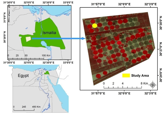
Figure 1.
Location map of the study area, Ismailia governorate, Egypt, overlaid with sentinel-2 image (false colour composition: NIR, Red, Green) acquired on 9 March 2022.
The field investigation of the site before reclamation showed that, generally, the studied soil has sandy loam texture with an average electric conductivity (ECe) 3.1 dS m−1, low value of organic matter (OM), and pH value around 7.8.
2.2. Field Data
2.2.1. Soil Samples
Thirty-three surface soil samples were collected based on the classification results of Landsat 8 of operational land images (OLI) acquired before plantation. The satellite data were used to produce an Enhanced Vegetation Index (EVI) map, which incorporated an “L” value to adjust for canopy background, “C” values as coefficients for atmospheric resistance, and values from the blue band. The map was classified into different categories based on the EVI values, and then the locations of the soil samples were allocated by symmetric random sampling. Twenty soil samples were also collected before plantation, and another thirteen soil samples were collected in the different soil zones, during the second growth stage after sixty days from plantation. Yield samples were collected as symmetric sampling grid contains 37 locations used to obtain a yield map of peanut. An area about 1 m2 was sited in each location, and then the peanut was weighed. The yield measured as kg peanut per m2 and then converted to tons per hectare.
Soil properties were described insitu [40]. Particle size distribution was carried out using Hydrometer Method [41]. The soil physical and chemical characteristics of collected soil samples (Table 1) were described insitu and were determined according to [42]. Electrical Conductivity (ECe) was determined in soil paste extract expressed in dS m−1. Soluble cations (Ca2+, Mg2+, Na+, K+) and anions (Cl−, CO32−, and HCO3−) were measured in the soil past extracts by titration [34,35]. Available Potassium was measured by Flame Photometer after extraction by Ammonium Acetate at pH 7 [43,44]. Micronutrients were determined by Atomic absorption spectrophotometer after extraction by Ammonium Bicarbonate-DTPA at pH 7.6 [44].

Table 1.
(a) Soil and Climate Evaluation Criteria of peanut crop [38,39,40,41,44,45]. (b) Field management practice of peanut crop.
Sodium Absorption Ratio (SAR) was calculated using:
Exchangeable Sodium Percentage (ESP) values were estimated based on SAR value as:
2.2.2. Deriving of Soil Productivity Maps
The measured soil characteristics such as soil salinity (ECe) dS m−1, soil texture expressed in sand (%), silt (%) and clay (%), soil pH, organic matter content (mg kg−1), calcium carbonate (%), and agro-metrological data of the selected area were used in evaluating soil productivity [45].
Soil and agro-metrological evaluation criteria were used as the inputs of SMCE in ILWIS software. ILWIS package is opensource software and can be downloaded free of charge from “http://52north.org/” (accessed on 30 May 2018). The SMCE was used to calculate soil suitability based on the crop requirements and using rank sum statistical analysis method as a combination rule [38,39,40,41].
Data processing into SMCE included several phases (Figure 2). First, all gathered soil samples were analyzed and then converted to soil maps using simple kriging spatial interpolation technique [42,43]. Second, the input layers were rasterized to cell size 30 min order to make an effective weighted overlay as the resolution of all the factor maps were not same. Third, the ranges of suitability for each soil class were determined while ordering soil layers into different criteria groups were selected to express the importance of each factor relative to other factor effects on crop yield [38,39,40,41,44,45,46]. The criteria groups were salinity, fertility (available K, P, Fe, Mn, and Zn), topography, soil physical characteristics, and climate (Table 1). Fourth, the criteria factors and the criteria constraints were selected [47,48], and the excluded areas were considered as constraints such as outside the boundary of the pivot and very saline soils.
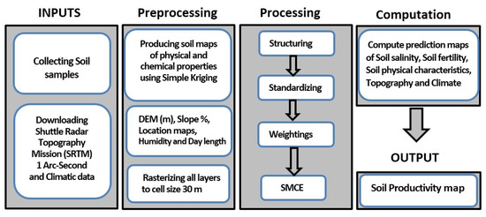
Figure 2.
Procedural flowchart for soil productivity through Spatial Multicriteria Evaluation.
Then, the factors in the five groups were defined [48]. The fifth step was data standardization for all the factors into units, enabling comparing and multiplying processes in the SMCE model [41,44,45]. Finally, Spatial Multi Criteria Evaluation approach was used to overlaying different attribute layers according to crop requirements using ranking sum equation as a combination rule; moreover, the output maps were reclassified into four productivity levels including high production, good production, moderate production, and low production [49,50,51,52].
2.2.3. Field Management Practices—Salhiya Site
The field investigation in Peanut pivot, Salhiya area, showed that the farm depends on irrigation system by adding fertilizer rates based on results of previous research. The fertigation program includes adding 107 Nitrogen units per hectare divided equally into three dates: first application after plantation, 15 days after plantation, and 30 days after plantation (Table 1). The Nitrogen units were applied as ammonium sulfate form (20.6% of Nitrogen). Additionally, the application rates of other fertilizers were, namely, 55 kg ha−1 super phosphates (15% of P2O5), 42 kg ha−1 of potassium sulfate (48% of K2O), and micro elements in 0.5 g L−1 concentration mixed form. Super phosphates and potassium sulfate were added as a soil application during land preparation and before plantation. The micronutrients were Fe, Zn, and Mn in combination (1, 1.5, 1, respectively); they were added twice with rates 715 L ha−1 and 950 L ha−1, respectively. Moreover, peanuts were planted after moisturizing the soil using a planter machine which delivered 5 seeds per 30 cm of row with 15 cm depth. The pivot takes 12 h to complete 1cycle where the pump station produces a pressure about 6 bars to maintain water flow of approximately 80 L per second through the center pivot nuzzles. The tillage practices were performed in the pivot area using pre-blow before plantation and the ridge after plantation to format the peanut lines in 40 cm width and 30 cm depth. Saline areas were identified using the ECe map and the satellite data acquired before plantation, then treated using additional subsurface plough and tillage in order to break any subsurface hard pans in 40 cm depth.
2.3. Statistical Analyses
The collected soil data and final yield were analyzed by the following statistical methods:
- A.
- A simple correlation procedure was applied by computing simple correlation coefficients matrix between peanut yield and soil characteristics [53]. Correlation analysis is utilized to quantify the degree to which yield data and soil variables are related.
- B.
- Multiple linear regression (MLR) accompanied with (R2), which refers to partial coefficient of determination, was calculated for yield to evaluate the relative contribution of each of soil properties and to simulate the prediction model for peanut yield (Y) with a measure of goodness of fit.
- C.
- Multiple Linear Regression analysis using a Stepwise selection procedure was used to determine each variable accounting for the yield variability majority as, multiple linear regression involves the fitting of a response to more than one predictor variable [53]. The stepwise selection method can be a forward, backward, or mixed selection method. In the current study, stepwise forward selection method computed a sequence of multiple linear regressions in the iterations of stepwise procedure by adding one variable predictor to the prediction equation at each stage of the procedure similar to a forward selection procedure. The tradeoff or eliminating variable to obtain another for the extra computational effort is the capacity to erase non-significant indicators as variables are added in addition to the ability to include new indicators taking after erasure. The additional variable was the one which incited the best diminishment in the error total of squares. It was additionally the variable which had the most partial correlation with the one of the soil properties as a dependent variable for fixed estimations of those variables included. In addition, it was the variable which had the highest F value.
- D.
- Ranking sum equation was used to manipulate weights for ranked soil criteria [22,24]. It calculates a ranked weight for a number (n) of different criteria (k) using Equation (3). Table 2 shows the weight vectors for various numbers of criteria according to Equation (1):where, n is number of criteria, wk is the weight, and k the criteria meaning that w1 ≥ w2 ≥ … ≥ wn ≥ 0.
Table 2. Criteria weights based on ranking sum equation.
2.4. Kriging
All gathered soil samples were analyzed and then converted to soil maps using simple kriging spatial interpolation method. Kriging is one of the best linear unbiased predictors that can be smoothed or correct relying upon the error estimation model [53]. Kriging is a generic name for a group of generalized least-squares regression models, utilized as a part of the pioneering work [53]. Many kirging methods are univariate geo-statistical algorithms such as simple kriging and ordinary kriging, where the kriging multivariate algorithms such as ordinary co-kriging and co-located co-kriging. All kriging predictors are variations of the general Equation (4) as follows:
where μ is a known stationary average, assumed to be steady over the entire domain and counted as the mean of the data [53]. The parameter λ is kriging weight; n is the point number of the selected samples used to make the interpolation; and μ(x0) is the samples average. The prediction of simple kriging is based on Equation (4) but with a slightly mathematical changes and modifications leading to Equation (5) as:
where the parameter μ(x0) in Equation (4) is modified by the stationary average μ in Equation (5). The samples number used to make the prediction in Equation (5) is calculated by the range of impact of the semivariogram [53].
Simple kriging was used for interpolating the soil characteristics to produce digital soil maps for the study area. Basically, SMCE model contain two main criteria constraints and factors. Outbound the study area, tracks and roads were considered as constraints; while the factors were represented by spatial maps. The spatial maps were divided into different classes using the optimum conditions for peanut crop [37,40]. Moreover, the spatial maps were standardized and converted to units that can be compared [54]. This step was necessary for applying the weighted linear combination algorithm in SMCE model [55]. In this study, the factor maps were ranked according to results of the stepwise regression model parameters. Moreover, the digital soil layers and other maps were rasterized with cell size as 30 m same as the digital elevation model and slope layers.
2.5. Accuracy Assessment of Mapping Peanut Productivity
Confusion matrix of 3 × 3 cells was selected to assess the accuracy of the GIS map of soil peanut productivity, producers and user’s accuracy of map unit, as well as the entire map. This accuracy assessment was based on KHat statistics and is a measure of agreement of accuracy. This measure of agreement is based on the difference between the actual and correct of confusion matrices classification. In this matrix, the column represents the omission errors, while the errors of commission are shown in the rows. Therefore, the confusion matrix enabled determining the omitted or under-estimated classified pixels and overestimated classified pixels of the different classes of soil. The interpretation of confusion matrix indicted that 37 testing points were used to perform the classification accuracy of the soil peanut productivity map, while the categorical accuracy of information classes was tested by different number of zone tests. However, according to the confusion matrix data, the overall accuracy (Po) had the value of 86.49%, which was calculated as follows:
where Po is the overall accuracy, r is the number of rows and columns in error matrix, Xii is the observation in row i and column i, while the overall Kappa Statistics are calculated by the following equation:
where r is the number of rows and columns in error matrix, N is the total number of observations (pixels), Xii is the observation in row i and column i, = is the marginal total of row i, and = is the marginal total of column i.
3. Results and Discussion
3.1. Soil Properties
3.1.1. Morphological, Physical, and Chemical Attributes
The studied soils represent the old deltaic plain of flat topography with an average elevation 15.3 m having a level to slightly level slope that ranges from 0.5 to 2.0%. The soil is well drained with a deep water table. The results of the morphological description of the studied soils indicated that the soil color varies from yellow to dark brown in soil samples at dry conditions, and it turned to yellow to very dark brown or yellowish brown with different degrees (light, moderate, dark) in moist conditions. Soil texture varies from sandy clay to sandy clay loam texture with slight variations in clay content. The soil structure in many samples was slightly hard to medium coarse in few samples with few types of gravel. The soil consistency was sticky and slightly plastic. Most of the soil samples had low and sometimes moderate effervescence with hydrochloric acid (HCl).
The data of physical and chemical properties of the soil samples collected before plantation are presented in Table 3. The analysis showed that clay content ranged from 28 to 41% in the surface soil samples, while sand content ranged from 48 to 64% with an average of about 53.7%. The texture class of the surface layers down to a depth of 40 cm is generally sandy clay and sandy clay loam in the western part of the pivot with an area about 13.9 hectare (Figure 3).
Table 3.
Physical characteristics of the study soil locations before plantation.
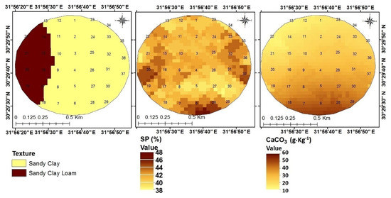
Figure 3.
Soil Texture, Saturation Percentage (SP), and CaCO3.
Values of saturation water percentage SP are relatively high and varied from 38% to 48%, which reflects a relatively high clay content and the sandy clay and sandy clay loam texture classes, these results agree with the results who indicated that El-Salhiya area characterized by clay loam, sandy loam, sand, and sandy clay loam texture [56]. Calcium carbonate is present in all of the studied samples with percentages varying from 0.59 to 6.1% and an average value about 2%. Digital maps of soil physical properties were categorized into suitable classes and used to identify soil units [39,40,43]. Soil texture maps were categorized into two classes, Sandy Clay Loam and Sandy Clay, in most of the pivot area. In addition, the results showed that the soil contains a low amount of CaCO3, which was categorized into two classes. i.e., above 3% and less than 3%,and represents most of the pivot area. The Saturation Percentage (SP) values obtained from soil analyses were categorized into three classes, i.e., below 43%, 43–45%, and above 45% as shown in Figure 4.
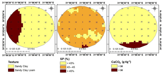
Figure 4.
Soil classes of Texture, Saturation Percentage (SP), and CaCO3.
Table 4 shows the chemical characteristics of the study soil locations before plantation. It indicates that the soils are mostly slightly to very slightly saline where the ECe values were relatively low, with no depth-wise distribution pattern. The results showed that ECe values varied from 1.94 to 6 dS m−1 with an average of 2.97 dS m−1. Generally, the soil has low to medium organic matter content ranging from 0.5 to 2.3%. Moreover, Exchangeable Sodium Percentage (ESP) values ranged from 1 to 12 with an average 6.33. On the other hand, Chloride (Cl−) is the dominant anion followed by Bicarbonate (HCO3−), and Carbonate (CO32−) was not found. Chloride anions ranged from 8.78–14.24 meq L−1, while the carbonates ranged from 1.26–3.12 meq L−1 with an average of 1.68 meq L−1.
Table 4.
Soil chemical characteristics of the study soil locations.
The cations and anions analyses indicated that the Potassium (K) represented the dominant cation, followed by Sodium (Na), then Calcium (Ca), and Magnesium (Mg) was the lowest one, as shown in Table 4. The dominance of Na+ ions may affect the Phosphorus (P) solubility if compared with Ca ions.
Moreover, the data in Table 4 and Figure 5 reveal that the studied soil samples have relatively medium pH values varying from 7.1 to 8.2 with an average value of 7.5. In the meantime, Potassium (K) ranged from 29.96–93.84 meq L−1. Sodium cation Na+ varied from 2.73–12.97 meq L−1. Calcium (Ca) and Magnesium (Mg) ranged from 0.42–4.43 meq L−1 and 0.09–2.29 meq L−1, respectively. On the other hand, Chloride Cl is the dominant anion, followed by Bicarbonate HCO3, and Carbonate CO3 was not found. The Chloride anion ranged from 8.78–14.24 meq L−1, while Bicarbonates varied from 1.26–3.12 meq L−1 with an average 1.68 meq L−1. A digital map of the electrical conductivity of soil paste extract (ECe) was categorized into three classes based on the effect of a range of electrical conductivity (ECe) levels on plant growth. The ECe classes were non-saline, weakly saline, and moderately saline, ranging from <2 dS m−1, 2–4 dS m−1, and >4 dS m−1, respectively [48]. The non-saline soil was located in the western part of the pivot, while most of the other area was weakly saline. The moderately saline area with values more than 4 dS m−1 located in the center of the pivot may be due to the soil slope in that area. In Figure 6, the pH levels were classified into three categories, namely, less than 7.2, 7.2–7.6, and 7.6–8.2, which may affect the availability of some nutrients. In addition, the pH level ranged from 7.6 to 8.2 in the eastern part of the pivot area. The ESP was generally below 15 indicated that, generally, the soils are not sodic soils, although they contain three different classes: below 7%, 7–10%, and above 10% [48]. The ESP class contains values below 7 located in the out boundaries of the pivot, while the ESP class ranged between a 7 and 10% spread in most of the pivot area.
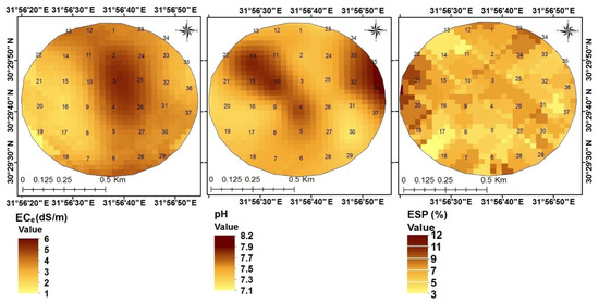
Figure 5.
Soil ECe, pH, and ESP of the study soil locations before plantation.
Figure 6.
Soil classes of ECe, pH, and ESP of the study soil locations before plantation.
3.1.2. Contents of Available Nutrients in the Site
The amounts of available Phosphorus, potassium, and micronutrients (Fe, Mn, and Zn) of the studied soil samples before plantation are shown in Table 5 and Figure 7 and Figure 8. The available potassium content varied from 228.5 to 384.8 mg kg−1soil. The highest values were found in the northern part of the pivot, whereas the lowest values were in the south part. In addition, a relative decrease was found around the external boundaries of the pivot. Available Phosphorus content is low and found in the range of 6.5 to 8.8 mg kg−1soil, slightly lower in center of the pivot. Soil pH values higher than 6.5 could limit the availability of Phosphorus in the soil. The micro-nutrients’ composition of the soil samples followed a pattern characterized by the dominance of Mn followed by Fe and Zn. In the meantime, Iron content ranged from 1.5 to 8.8 mg kg−1soil with a mean of 3.5 mg kg−1soil. The higher Fe value characterizes the eastern part of the pivot, while the lowest value is in the northwest of the pivot. The results showed very high variation in the amount of available Manganese, which ranged from 0.3 to 8.3 mg kg−1soil with an average of 4.3 mg kg−1soil, reflecting generally adequate values for plant growth. Generally, the results of the soil sample analysis showed that the amount of available Zinc ranges between 0.10 and 1.8 mg kg−1soil with an average of 0.6 mg kg−1soil, indicating low Zn availability. The soil pH values higher than 6.5 could limit the availability of Zinc, and the pivot areas with high ECe values may affect it, where the high salt saline soils diminish the Zinc availability.
Table 5.
Available P, K, and micronutrients (Fe, Mn, and Zn) of the soil samples.
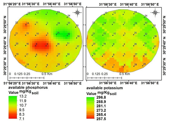
Figure 7.
Available Phosphorus and potassium of the study soil locations.
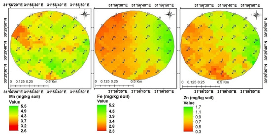
Figure 8.
Available Fe, Mn, and Zn of the study soils in the Salhiya Site.
3.1.3. Salhiya Digital Soil Maps of Available Nutrients and Soil Units
The data of the soil characteristics and the available P, K, Fe, Mn, and Zn of soil samples collected from different location of the studied pivot were classified [48]. Available P data were classified in three classes (Figure 9) as high (<12 mg kg−1soil), medium (between 10–12 mg kg−1soil), and low (10 mg kg−1soil) content [43]. However, available P use efficiency may have influenced by many factors related to P fertilizer, the crop grown, and mainly to the soil pH, the content of CaCO3, and clay.
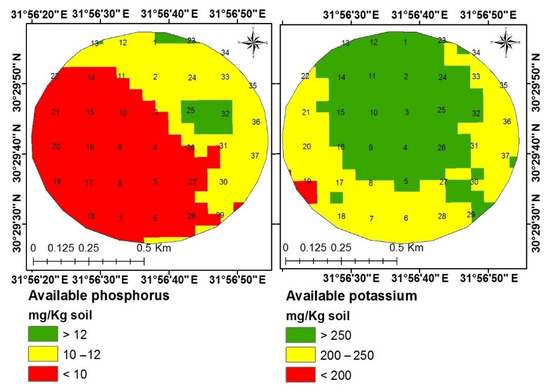
Figure 9.
Soil classes of available Phosphorus (P) and available potassium (K).
The data of available K were arranged in three classes (Figure 9) as high content (more than 250 mg kg−1soil), medium content (from 200–250 mg kg−1soil), and low content (less than 200 mg kg−1soil) [43]. The available Iron was arranged in three classes (Figure 10), namely, high content (more than 4 mg kg−1soil), medium content (between 2 to 4 mg kg−1soil), and low content (less than 2 mg kg−1soil) [57]. In general, Iron (Fe) and micronutrient use efficiency may have been influenced by some factors such as soil pH and the content of CaCO3, OM, and clay. Available manganese was categorized into two classes as high content, “more than 1.5 mg kg−1soil”, and medium content, “ranged from 1–1.5 mg kg−1soil” [57]. Furthermore, available zinc (Zn) was categorized into two classes (Figure 10), medium and low; the medium class contains available zinc (Zn) more than 1.8 mg kg−1soil,and the low class contains available zinc less than 1.8 mg kg−1soil.
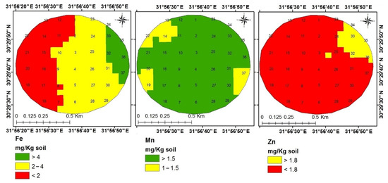
Figure 10.
Soil classes of available Iron (Fe), Manganese (Mn), and available Zinc (Zn).
A digital soil units map was obtained usinganoverlay technique by combining the classified maps of the studied soil properties (texture, ECe, pH, CaCO3, SP, and ESP). The output layer of the digital soil map unit showed four soil map units having some different characteristics. Table 6 and Figure 11 shown the soil map units characterized by the following [42]:
Table 6.
Area of different units based on soil properties.
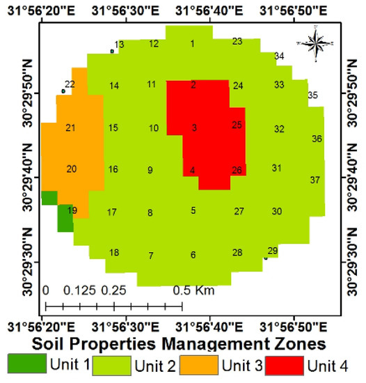
Figure 11.
Different soil units based on soil factors.
- Soil unit 1 is characterized by non-saline soil with ECe ranging from 0 to 2 dS m−1, low % CaCO3 less than 3%, and sandy clay loam texture.
- Soil unit 2 is characterized by non-saline ECe, sandy clay, and low CaCO3.
- Soil map unit 3 is characterized by very slightly saline ECe ranging from 2–4 dS m−1, low CaCO3, and sandy clay loam texture.
- Soil map unit 4 is characterized by slightly saline soil with ECe more than 4 dS m−1, low CaCO3 content, and sandy clay loam texture.
In the meantime, the overlay technique was used to combine the soil classified maps of available P, K, Fe, and Mn. The output of overlay layers contained six soil fertility management zones, differing from each other with the area of different soil management zones. The results of Figure 12 also show soil units based on fertility level in the following descending order:
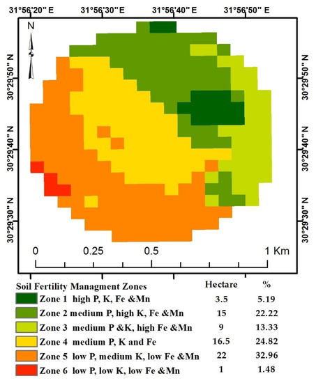
Figure 12.
Different soil units based on some soil characteristics.
- Zone 1: this area represents soils having a high content of available Phosphorus, Potassium, Iron, and Manganese.
- Zone 2: this area had fair amounts of soil fertility elements with high soil content of available K, Fe, Mn and medium soil content of available P.
- Zone 3: this area had a flat elevated area with medium soil content of available P and K in addition to high soil content of available Fe.
- Zone 4: characterized by a flat area with medium soil content of available Phosphorus, medium soil content of available K, and medium soil content of available Fe.
- Zone 5: relatively elevated soils and contains low content of most soil fertility elements such as available Phosphorus, low Fe, and moderate amount of available K.
- Zone 6: characterized by nutrient stress due to the low contents of most fertility elements such as available P, K, and Fe with high elevated soils.
Finally, both layers of soil properties and soil fertility management zones were combined to give one combined management zone. The results of the overlay layers show six management zones, as shown in Figure 13, with varied total areas, namely, rich nutrient area occupied about 24%of the pivot(16 ha from the total area of the pivot), very good area about 9% (6 ha), good area around 5% (3 ha), normal area occupied 28% (19 ha), moderate area occupied 33% (22 ha), and poor area around 3% (1 ha).
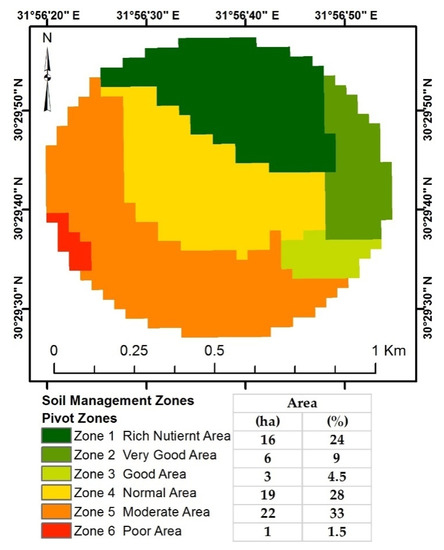
Figure 13.
Total areas of final management zones map based on soil properties and soil fertility management zones.
Yield is a powerful criterion to determine management zones within a field due to the wide yield variation levels in farms. The results showed that the rich nutrient area containing the highest yield was in zone one around 3.5 to 3.7 ton ha−1. For the yield in the second zone, the very good area varied between 3.2 and 3.4 ton ha−1. Additionally, the good area zone was located in the yield level between 2.9 and 2.1 ton ha−1. For the yield in zone four, the normal area contained 22 hectares located in yield level ranged between 2.7 and 2.8 ton ha−1.
3.1.4. Correlation between Peanut Yield and Soil Characteristics
A simple correlation matrix of some soil characteristics are presented in Table 7, namely, Texture, ECe, soil pH, organic matter, saturation percentage, CaCO3, Kavailable, Pavailable, Fe, Mn, and Zn. The regression analyses for peanut yield and soil characteristics are presented in Table 8. Basically, the result indicated that SP performed better than OM, CaCO3, ECe, and pH for predicting peanut yield with correlation coefficient 0.77, 0.73, 0.60, 0.54, and 0.40, respectively.
Table 7.
Simple correlation matrix of some soil characteristics.
Table 8.
Correlation between yield (ton ha−1) and soil characteristics.
Generally, soil plays a great role in yield production, where it is the main path for water and nutrient supply needed to complete photosynthesis process. The multiple linear regression analysis using stepwise selection procedure was used to asses to determine the main soil variables (ECe, pH, CaCO3, OM, and SP) accounting for the yield variability majority. The results of the statistical analysis using the stepwise multiple linear regression for the different soil variables to predict the final yield production using ECe, pH, CaCO3, OM, and saturation percentage are demonstrated in Figure 14 and Table 9.
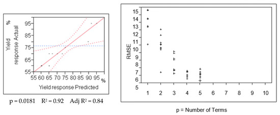
Figure 14.
Actual yield by predicted yield response and Root Mean Squared Error (RMSE). Coefficient of determination (R2), adjusted R2 and p value of the prediction model is reported below the plot. The diagonal red line represents the linear fit of the input data. The dotted red linesare the data range. The dotted blue horizontal line is the mean.
Table 9.
Results of the stepwise MLR analysis for soil characteristics and correlation between model parameters and measured yield.
The statistical analysis showed high correlation between ECe and the calculated yield. The result showed high R2 around 0.92 for the predicted values of the crop coefficient. The result from the prediction equations were used to predict and map the peanut yield. The result shows a correlation between the calculated yield and predicted yield for ECe, pH, CaCO3, and OM were significant, as presented in Table 9.
The result showed that the yield estimations have a good agreement with field measurements with significant correlation coefficient, where soil maps were successfully employed on yield prediction. Furthermore, the results showed high R2 for the predicted values of crop coefficient 0.92 and 0.85, respectively. It indicates that the estimation of crop yield using remote sensing data is essentially significant. However, R2 values of the correlation between the calculated and predicted yield in the model combining ECe, pH, OM, and SP were higher than separated or one-factor models.
3.2. Soil Productivity Assessment
3.2.1. Mapping Soil Productivity
Soil maps were processed to produce soil attribute values that were used as a pre-data for a soil productivity model built in ILWES using SMCE. The SMCE soil model classified the studied area into four production soil classes: high production soil with an average production around 3.50 ton ha−1, a good production soil with an average production of 3.20 ton ha−1, moderate production soil with an average production of 2.90 ton ha−1, and, finally, low production soil with an average production around 2.50 ton ha−1. Figure 15 shows the production levels and the representing areas for each class. The classes areas were 35%, 21%, 38%, and 6% of the study area, respectively. The results indicated that high production areas were found generally in soil of ECe from 0.3 to 3.9 dS m−1, soil pH level (7.1 to 7.8), available potassium (20 to 30 mg kg−1), Iron (1 to 2.3 mg kg−1), Manganese (1.7 to 2.4 mg kg−1), and CaCO3 that ranged from 1.1 to 4.3 g kg−1 (Table 10). Low production areas were characterized by low fertility and ECe between 1.3 and 5.2 dS m−1, soil pH levels between 7.7 and 8.2, and available potassium (1.5 to 1.6 mg kg−1), iron (0.9 to 0.5 mg kg−1), Manganese (1.1 to 0.2 mg kg−1), and CaCO3 (5.6 g kg−1). Comparing these results with the peanut crop requirements in terms of soil topography and climate conditions indicated that the area is generally good soil for cultivating peanut crop; however, the low production areas need to be enhanced by adding a sufficient amount of organic matter.
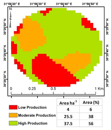
Figure 15.
Soil productivity of the studied pivot.
Table 10.
Soil characteristics of high and low crop production.
3.2.2. Accuracy Assessment of Mapping Peanut Productivity
The mapping accuracy of the mapping units of high, moderate, and low production were assessed by 14, 12, and 11 zone tests, respectively (Table 11). Clearing that, the second row showed that only three zone tests (3 × 3 × 3 pixels) were overestimated and classified in higher information class (class of moderate production) while they really belonged to the class of low production (Table 12). Moreover, a zone test of the class of high production was omitted (underestimated) to be a member in lower class information (class of moderate production), where the correctly classified pixels of all information classes are represented along the diagonal of the confusion matrix (Table 12).
Table 11.
Confusion matrix of soil productivity output classification.
Table 12.
Producer and user’s accuracies of soil productivity output data classification.
However, according to the confusion matrix data, overall accuracy (Po) had the value of 86.49%, which was calculated as follows:
Po= (32/37) × 100 = 86.49%, while the overall Kappa Statistics had the value of 79.8%:
where r is the number of rows and columns in error matrix, N is the total number of observations (pixels), Xii is the observation in row i and column i, is the marginal total of row i, and = is the marginal total of column i.
The number of the omitted and committed pixels was related to all pixels to calculate the percentage of these errors. The summation of this percentage represented the erroneously classified pixels. Considering the categorical accuracy expressing the potential map units, we can calculate the producer accuracy and user accuracy of soil productivity for the classified output data, as shown in Table 13.
Table 13.
Classification accuracy assessment of different classes of peanut soil productivity.
The table showed that the producer’s accuracies ranged from 80.00 to 92.31%; the lowest producer’s accuracy was recorded in the case of low production class, while the highest producer’s accuracies was assigned to high production class. Moreover, the user’s accuracies ranged between 72.72% (class of low production) and 85.71% (class of high production). Moreover, the accuracy assessment of the soil productivity map showed adequate classification results with 86.49% overall accuracy and 79.8 overall kappa (Table 13). The results of the Kappa factor show a significant effect between the different classes on the model of output maps.
3.3. Nitrogen Management Zones
The field investigation in Peanut pivot in the Salhiya area showed that the farm depends on fertigation system by adding fertilizer rates based on the results of the previous research. The investigation also declared that the farm manager used to add 107 Nitrogen units per hectare divided equally into 3 dates, first day after plantation, 15 days after plantation, and 30 days after plantation, which agreed with previous research suggesting the use of 107 units of actual Nitrogen per hectare in reclaimed areas to achieve economically effective yields. The authors indicated that direct Nitrogen applications are not generally needed for peanut. However, Nitrogen applications increase the final yield in sandy soils and new reclaimed areas without high peanut nodulating and the deficiency of Nitrogen is obvious; these areas often respond to applications of the Nitrogen [58]. The fertigation system spread the fertilizer applications equally in the pivot area. However, the results of NDVI maps—produced from Landsat imagery acquired after 60 days of plantation—show different units with high values, moderate values, and low values. Comparing the results of NDVI maps with nitrogen uptakes with the plants declare that the low NDVI values are located in areas where the deficiency in Nitrogen is obvious.
Data of the soil such as soil texture, soil type, elevation of the landscape, and slope allow for sampling the study area into similar classes and in smaller units along the crop productivity map. The explanation of Nitrogen heterogeneity within the pivot appeared after overlapping the topography map with the NDVI map, where, in the high slope areas, a Nitrogen deficiency exists (Figure 16).
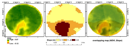
Figure 16.
Overlapping map of Average seasonal NDVI and slope in the study area.
The results indicate that the areas with high slope are usually classified as weak vegetation growth areas with an average NDVI of 0.3 to 0.35 and low predicted Nitrogen (Figure 16). Furthermore, the areas with moderate slope are often classified as moderate vegetation growth areas with an average NDVI of 0.35 to 0.55 and normal predicted Nitrogen. The results also declared that the areas with low slope are often classified as healthy vegetation growth areas with an average NDVI of 0.55 to 0.80 and high predicted Nitrogen.
In traditional agriculture practices, nutrient application is usually added to the whole pivot area in the same amounts, but with the help of the final GIS management zones map, a varied amount of nutrients can be added to different pivot zones. Six different application rates were recommended, correlated with management zones. The recommendation rates for phosphorous and potassium nutrients are descripted for soil zones in Table 14 and Table 15. Additionally, the result of Phosphorus application showed that using variable rate technology (VRT) and according to the current fertilizers price; in traditional agriculture, the fertilizer application of 55 (P) kg ha−1 was equal to 367 kg super phosphate, which costs EGP 1310 per hectare and around EGP 100,800.0 for the total pivot area (Table 14). The total costs with site-specific application were EGP 70,346.0.
Table 14.
Amounts and costs of Phosphorus application using VRT.
Table 15.
Amounts and costs of potassium application using VRT.
Table 15 show the result of potassium application using VRT and according to the current fertilizer price; in traditional agriculture, the fertilizer application of 42 (K) kg ha−1 equal to 130 kg potassium sulphate costs EGP 1400 Egyptian pound per hectare and around EGP 94,500.0 for the total pivot area, while total potassium fertilizer costs with site-specific applications were EGP 80,168.0.
In addition, both tables described the varied rates in nutrients recommendations for the whole pivot area. Comparing the traditional agriculture practices and the precision farming practices, we can reduce the use of super phosphate by 0.23, 0.20, 0.17, 0.14, and 0.05 tons in soil zones 1, 2, 3, 4, and 5, respectively, while zone 6 was fully supplied with super phosphate. Additionally, potassium application was reduced by 0.34, 0.34, 0.31, 0.30, 0.29, and 0.29 tons in soil zones 1, 2, 3, 4, and 5, respectively, concluding that the variable fertilizer application rate helped to save total amounts of 0.74 and 0.13 tons of super phosphate and potassium sulphate, respectively, in addition to protecting the soil and the environment for the whole experimental pivot area.
4. Conclusions
The conclusion drawn from this study indicates that GIS techniques with abundant information on soil properties in the study site contributed to determining the spatial pattern of crop growth changes. Variations in soil characteristics had a significant impact on peanut yield, and this was predicted in the soil suitability model. The spatial multi-criteria soil model was able to achieve good accuracy by using a good spatial distribution of soil samples. The multiple linear regression growth model was able to predict the productivity of the peanut crop when using adequate data of soil characteristics at different field zones, which indicates positive capabilities for use in predicting and analyzing crop yield variations in the specific locations of the field. Compared with the crop growth models, the soil suitability model provided better detection of small areas referring to soil properties, such as calcareous areas and saline soils. Moreover, the resulting yield estimations showed a good agreement with field measurements with significant correlation coefficient. The objective was to contribute to policymaking in a specific field in order to furnish an evaluation about the transformations at a territorial scale and for studying the strategies to realize environmental sustainability and to reduce the territorial impacts.
Author Contributions
Conceptualization, M.M.E., A.E.A.S.S., P.D., M.S.A. and A.S.; methodology, M.M.E., A.E.A.S.S., P.D. and M.S.A.; software, M.M.E., A.E.A.S.S., P.D., M.S.A. and A.S.; validation, M.M.E., A.E.A.S.S. and M.S.A.; formal analysis, M.M.E., A.E.A.S.S., P.D. and M.S.A.; investigation, M.M.E., A.E.A.S.S., M.S.A. and A.S.; resources, M.M.E., A.E.A.S.S., P.D., M.S.A. and A.S.; data curation, M.M.E., A.E.A.S.S., P.D., M.S.A. and A.S.; writing—original draft preparation, M.M.E., A.E.A.S.S., P.D., M.S.A. and A.S.; writing—review and editing, M.M.E., A.E.A.S.S., P.D., M.S.A. and A.S.; visualization, M.M.E., A.E.A.S.S., P.D., M.S.A. and A.S.; supervision, M.M.E., A.E.A.S.S., M.S.A. and A.S.; project administration, M.M.E., A.E.A.S.S., P.D., M.S.A. and A.S. All authors have read and agreed to the published version of the manuscript.
Funding
This research received no external funding.
Institutional Review Board Statement
Not applicable.
Informed Consent Statement
Not applicable.
Data Availability Statement
Not applicable.
Acknowledgments
The manuscript presented a scientific participation between the scientific institutions in two countries (Egypt and Italy). The authors are grateful to scientific Institution of two Countries for their support in carrying out the work.
Conflicts of Interest
The authors declare no conflict of interest.
References
- Ratnaparkhi, S.; Khan, S.; Arya, C.; Khapre, S.; Singh, P.; Diwakar, M.; Shankar, A. Smart agriculture sensors in IOT: A review. Mater. Today Proc. 2020. [Google Scholar] [CrossRef]
- Chandra Pandey, P.; Tripathi, A.K.; Sharma, J.K. An evaluation of GPS opportunity in market for precision agriculture. In GPS and GNSS Technology in Geosciences; Petropoulos, G.P., Srivastava, P.K., Eds.; Chapter 16; Elsevier: Oxford, UK, 2021; pp. 337–349. [Google Scholar] [CrossRef]
- Corwin, D.L.; Lesch, S.M.; Oster, J.D.; Kaffka, S.R. Monitoring management-induced spatio–temporal changes in soil quality through soil sampling directed by apparent electrical conductivity. Geoderma 2006, 131, 369–387. [Google Scholar] [CrossRef]
- Castrignano, A.; Giugliarini, L.; Risaliti, R.; Martinelli, N. Study of spatial relationships among some soil physico-chemical properties of a field in central Italy using multivariate geostatistics. Geoderma 2000, 97, 39–60. [Google Scholar] [CrossRef]
- Pecze, Z.; Neményi, M.; Mesterházi, P.Á.; Stépán, Z. The Function of the Geographic Information System (GIS) in Precision Farming. In Proceedings of the IFAC/CIGR Workshop on Artificial Intelligence in Agriculture 2001, Budapest, Hungary, 6–8 June 2001; Volume 34, pp. 15–18. [Google Scholar] [CrossRef]
- Buttafuoco, G.; Tallarico, A.; Falcone, G.; Guagliardi, I. A geostatistical approach for mapping and uncertainty assessment of geogenic radon gas in soil in an area of southern Italy. Environ. Earth Sci. 2010, 61, 491–505. [Google Scholar] [CrossRef]
- Vašát, R.; Heuvelink, G.B.M.; Borůvka, L. Sampling design optimization for multivariate soil mapping. Geoderma 2010, 155, 147–153. [Google Scholar] [CrossRef]
- Mylavarapu, R.S.; Lee, W.D. UF/IFAS Nutrient Management Series: Soil Sampling Strategies for Precision Agriculture 1. Florida, USA, 2002. Available online: https://edis.ifas.ufl.edu/publication/SS402 (accessed on 11 February 2022).
- Corwin, D.L.; Lesch, S.M. Characterizing soil spatial variability with apparent soil electrical conductivity. Part II. Case study. Comput. Electron. Agric. 2005, 46, 135–152. [Google Scholar] [CrossRef]
- Wang, J.; Sun, Z.; Cao, R. An efficient and robust Kriging-based method for system reliability analysis. Reliab. Eng. Syst. Saf. 2021, 216, 107953. [Google Scholar] [CrossRef]
- Jadidoleslam, N.; Mantilla, R.; Krajewski, W.F.; Cosh, M.H. Data-driven stochastic model for basin and sub-grid variability of SMAP satellite soil moisture. J. Hydrol. 2019, 576, 85–97. [Google Scholar] [CrossRef]
- Lark, R.M. Designing sampling grids from imprecise information on soil variability, an approach based on the fuzzy kriging variance. Geoderma 2000, 98, 35–59. [Google Scholar] [CrossRef]
- Issad, H.A.; Aoudjit, R.; Rodrigues, J.J.P.C. A comprehensive review of Data Mining techniques in smart agriculture. Eng. Agric. Environ. Food 2019, 12, 511–525. [Google Scholar] [CrossRef]
- Nelson, M.D.; Garner, J.D.; Tavernia, B.G.; Stehman, S.V.; Riemann, R.I.; Lister, A.J.; Perry, C.H. Assessing map accuracy from a suite of site-specific, non-site specific, and spatial distribution approaches. Remote Sens. Environ. 2021, 260, 112442. [Google Scholar] [CrossRef]
- Liu, F.; Rossiter, D.G.; Zhang, G.-L.; Li, D.-C. A soil colour map of China. Geoderma 2020, 379, 114556. [Google Scholar] [CrossRef]
- Owens, P.R.; Rutledge, E.M. Morphology. In Encyclopedia of Soils in the Environment; Hillel, D., Ed.; Elsevier: Oxford, UK, 2005; pp. 511–520. [Google Scholar]
- Huuskonen, J.; Oksanen, T. Soil sampling with drones and augmented reality in precision agriculture. Comput. Electron. Agric. 2018, 154, 25–35. [Google Scholar] [CrossRef]
- Vecchio, Y.; De Rosa, M.; Adinolfi, F.; Bartoli, L.; Masi, M. Adoption of precision farming tools: A context-related analysis. Land Use Policy 2020, 94, 104481. [Google Scholar] [CrossRef]
- McKinion, J.M.; Willers, J.L.; Jenkins, J.N. Spatial analyses to evaluate multi-crop yield stability for a field. Comput. Electron. Agric. 2010, 70, 187–198. [Google Scholar] [CrossRef]
- Lagacherie, P.; Buis, S.; Constantin, J.; Dharumarajan, S.; Ruiz, L.; Sekhar, M. Evaluating the impact of using digital soil mapping products as input for spatializing a crop model: The case of drainage and maize yield simulated by STICS in the Berambadi catchment (India). Geoderma 2022, 406, 115503. [Google Scholar] [CrossRef]
- López-Lozano, R.; Casterad, M.A.; Herrero, J. Site-specific management units in a commercial maize plot delineated using very high resolution remote sensing and soil properties mapping. Comput. Electron. Agric. 2010, 73, 219–229. [Google Scholar] [CrossRef] [Green Version]
- Li, M.; Shamshiri, R.R.; Schirrmann, M.; Weltzien, C.; Shafian, S.; Laursen, M.S. UAV Oblique Imagery with an Adaptive Micro-Terrain Model for Estimation of Leaf Area Index and Height of Maize Canopy from 3D Point Clouds. Remote Sens. 2022, 14, 585. [Google Scholar] [CrossRef]
- Lei, L.; Qiu, C.; Li, Z.; Han, D.; Han, L.; Zhu, Y.; Wu, J.; Xu, B.; Feng, H.; Yang, H.; et al. Effect of Leaf Occlusion on Leaf Area Index Inversion of Maize Using UAV–LiDAR Data. Remote Sens. 2019, 11, 1067. [Google Scholar] [CrossRef] [Green Version]
- Mourad, R.; Jaafar, H.; Anderson, M.; Gao, F. Assessment of Leaf Area Index Models Using Harmonized Landsat and Sentinel-2 Surface Reflectance Data over a Semi-Arid Irrigated Landscape. Remote Sens. 2020, 12, 3121. [Google Scholar] [CrossRef]
- Gaso, D.V.; de Wit, A.; Berger, A.G.; Kooistra, L. Predicting within-field soybean yield variability by coupling Sentinel-2 leaf area index with a crop growth model. Agric. For. Meteorol. 2021, 308–309, 108553. [Google Scholar] [CrossRef]
- Coops, N.C.; Waring, R.H.; Hilker, T. Prediction of soil properties using a process-based forest growth model to match satellite-derived estimates of leaf area index. Remote Sens. Environ. 2012, 126, 160–173. [Google Scholar] [CrossRef]
- Fastellini, G.; Schillaci, C. Precision farming and IoT case studies across the world. In Agricultural Internet of Things and Decision Support for Precision Smart Farming; Castrignanò, A., Buttafuoco, G., Khosla, R., Mouazen, A.M., Moshou, D., Naud, O., Eds.; Chapter 7; Academic Press: Cambridge, MA, USA, 2020; pp. 331–415. [Google Scholar]
- Leopizzi, S.; Gondret, K.; Boivin, P. Spatial variability and sampling requirements of the visual evaluation of soil structure in cropped fields. Geoderma 2018, 314, 58–62. [Google Scholar] [CrossRef]
- Lawes, R.A.; Robertson, M.J. Whole farm implications on the application of variable rate technology to every cropped field. Field Crop. Res. 2011, 124, 142–148. [Google Scholar] [CrossRef]
- Orhan, O. Land suitability determination for citrus cultivation using a GIS-based multi-criteria analysis in Mersin, Turkey. Comput. Electron. Agric. 2021, 190, 106433. [Google Scholar] [CrossRef]
- Ziadat, F.M. Land suitability classification using different sources of information: Soil maps and predicted soil attributes in Jordan. Geoderma 2007, 140, 73–80. [Google Scholar] [CrossRef]
- Jafari, S.; Zaredar, N. Land Suitability Analysis using Multi Attribute. Int. J. Environ. Sci. Dev. 2010, 1, 441–445. [Google Scholar] [CrossRef]
- Boote, K.J. Growth Stages of Peanut (Arachis hypogaea L.). Peanut Sci. 1982, 9, 35–40. [Google Scholar] [CrossRef]
- CBI Ministry of Foreign Affairs. The European Market Potential for Groundnuts. Available online: https://www.cbi.eu/market-information/processed-fruit-vegetables-edible-nuts/groundnuts/market-potential (accessed on 7 April 2020).
- Dobrescu, M.; Slette, J. Food and Agricultural Import Regulations and Standards Country Report. J. Off. 2020, 22, 22. Available online: https://apps.fas.usda.gov/newgainapi/api/Report/DownloadReportByFileName?fileName=Food%20and%20Agricultural%20Import%20Regulations%20and%20Standards%20Country%20Report_Cairo_Egypt_12-31-2020 (accessed on 9 April 2022).
- Ustaoglu, E.; Sisman, S.; Aydınoglu, A.C. Determining agricultural suitable land in peri-urban geography using GIS and Multi Criteria Decision Analysis (MCDA) techniques. Ecol. Modell. 2021, 455, 109610. [Google Scholar] [CrossRef]
- Samanta, S.; Pal, B.; Pal, D.K. Land Suitability Analysis for Rice Cultivation Based on Multi-Criteria Decision Approach through GIS. Int. J. Sci. Emerg. Technol. 2011, 1, 12–20. [Google Scholar]
- Holland, J.E.; White, P.J.; Glendining, M.J.; Goulding, K.W.T.; McGrath, S.P. Yield responses of arable crops to liming—An evaluation of relationships between yields and soil pH from a long-term liming experiment. Eur. J. Agron. 2019, 105, 176–188. [Google Scholar] [CrossRef] [PubMed]
- Ahmad, L.; Nabi, F. Introduction to Precision Agriculture. In Agriculture 5.0: Artificial Intelligence, IoT, and Machine Learning; CRC Press: Boca Raton, FL, USA, 2021; pp. 1–23. [Google Scholar] [CrossRef]
- Eppes, M.C.; Johnson, B.G. Describing Soils in the Field: A Manual for Geomorphologists. In Reference Module in Earth Systems and Environmental Sciences; Elsevier: Oxford, UK, 2021. [Google Scholar]
- Bouyoucos, G.J. Hydrometer Method Improved for Making Particle Size Analyses of Soils. Agron. J. 1962, 54, 464–465. [Google Scholar] [CrossRef]
- Soil Science Division Staff. Soil Science Division Staff. Soil survey manual. In USDA Handbook 18; Ditzler, C., Scheffe, K., Monger, H.C., Eds.; Government Printing Office: Washington, DC, USA, 2017. [Google Scholar]
- Sparks, D.L.; Page, A.L.; Helmke, P.A.; Loeppert, R.H.; Soltanpour, P.N.; Tabatai, M.A.; Johnston, C.T.; Summer, M.E. (Eds.) Methods of Soil Analysis-Chemical Methods; Soil Science Society of America, Inc.: Madison, WI, USA; American Society of Agronomy, Inc.: Madison, WI, USA, 1996; Volume 70, pp. 342–343. [Google Scholar]
- Soltanpour, P.N.; Khan, A.; Lindsay, W.L. Factors affecting DTPA-extractable Zn, Fe, Mn, and Cu from soils. Commun. Soil Sci. Plant Anal. 1976, 7, 797–821. [Google Scholar] [CrossRef]
- Rossiter, D.G. A theoretical framework for land evaluation. Geoderma 1996, 72, 165–190. [Google Scholar] [CrossRef]
- Walke, N.; Obi Reddy, G.P.; Maji, A.K.; Thayalan, S. GIS-based multicriteria overlay analysis in soil-suitability evaluation for cotton (Gossypium spp.): A case study in the black soil region of Central India. Comput. Geosci. 2012, 41, 108–118. [Google Scholar] [CrossRef]
- Carver, S.J. Integrating multi-criteria evaluation with geographical information systems. Int. J. Geogr. Inf. Syst. 1991, 5, 321–339. [Google Scholar] [CrossRef] [Green Version]
- FAO. A Framework for Land Evaluation; Soils Bulletin 32; FAO: Rome, Italy, 1976; p. 72. ISBN 92-5-100111-1. [Google Scholar]
- Wackernagel, H. Geostatistical models and kriging. IFAC Proc. Vol. 2003, 36, 543–548. [Google Scholar] [CrossRef]
- McBratney, A.B.; Mendonça Santos, M.L.; Minasny, B. On digital soil mapping. Geoderma 2003, 117, 3–52. [Google Scholar] [CrossRef]
- Vaidya, O.S.; Kumar, S. Analytic hierarchy process: An overview of applications. Eur. J. Oper. Res. 2006, 169, 1–29. [Google Scholar] [CrossRef]
- Saaty, T.L. Decision Making with the Analytic Hierarchy Process. Int. J. Serv. Sci. 2008, 1, 83–98. [Google Scholar] [CrossRef] [Green Version]
- Szulc, S. (Ed.) The correlation coefficient and regression lines. In Statistical Methods; Chapter 15; Pergamon: Oxford, UK, 1965; pp. 425–460. [Google Scholar]
- Malczewski, J. Ordered weighted averaging with fuzzy quantifiers: GIS-based multicriteria evaluation for land-use suitability analysis. Int. J. Appl. Earth Obs. Geoinf. 2006, 8, 270–277. [Google Scholar] [CrossRef]
- Ronald, E.J.; Wei-gen, J.; Peter, A. Raster procedures for multi-criteria/multi-objective decisions. Photogramm. Eng. Remote Sens. 1995, 61, 539–547. [Google Scholar]
- Farg, E.; Arafat, S.; Abd El-Wahed, M.S.; El-Gindy, A. Evaluation of water distribution under pivot irrigation systems using remote sensing imagery in eastern Nile delta. Egypt. J. Remote Sens. Sp. Sci. 2017, 20, S13–S19. [Google Scholar] [CrossRef]
- Lindsay, W.L.; Norvell, W.A. Development of a DTPA Soil Test for Zinc, Iron, Manganese, and Copper. Soil Sci. Soc. Am. J. 1978, 42, 421–428. [Google Scholar] [CrossRef]
- Feng, C.; Sun, Z.; Zhang, L.; Feng, L.; Zheng, J.; Bai, W.; Gu, C.; Wang, Q.; Xu, Z.; van der Werf, W. Maize/peanut intercropping increases land productivity: A meta-analysis. Field Crop. Res. 2021, 270, 108208. [Google Scholar] [CrossRef]
Publisher’s Note: MDPI stays neutral with regard to jurisdictional claims in published maps and institutional affiliations. |
© 2022 by the authors. Licensee MDPI, Basel, Switzerland. This article is an open access article distributed under the terms and conditions of the Creative Commons Attribution (CC BY) license (https://creativecommons.org/licenses/by/4.0/).