Article

Operational Data-Driven Intelligent Modelling and Visualization System for Real-World, On-Road Vehicle Emissions—A Case Study in Hangzhou City, China

1
Research Center for Air Pollution and Health, Key Laboratory of Environmental Remediation and Ecological Health, Ministry of Education, College of Environment and Resource Sciences, Zhejiang University, Hangzhou 310058, China
2
Bytedance Inc., Hangzhou 310058, China
3
College of Science and Technology, Hebei Agricultural University, Baoding 071000, China
4
Chinese Academy of Meteorological Sciences, China Meteorological Administration, Beijing 100081, China
*
Authors to whom correspondence should be addressed.
Sustainability 2022, 14(9), 5434; https://doi.org/10.3390/su14095434
Submission received: 16 February 2022 / Revised: 14 April 2022 / Accepted: 27 April 2022 / Published: 30 April 2022
(This article belongs to the Collection Air Pollution Control and Sustainable Development)

Abstract

:
On-road vehicle emissions play a crucial role in affecting air quality and human exposure, particularly in megacities. In the absence of comprehensive traffic monitoring networks with the general lack of intelligent transportation systems (ITSs) and big-data-driven, high-performance-computing (HPC) platforms, it remains challenging to constrain on-road vehicle emissions and capture their hotspots. Here, we established an intelligent modelling and visualization system driven by ITS traffic data for real-world, on-road vehicle emissions. Based on the HPC platform (named “City Brain”) and an agile Web Geographic Information System (WebGISs), this system can map real-time (hourly), hyperfine (10~1000 m) vehicle emissions (e.g., PM2.5, NOx, CO, and HC) and associated traffic states (e.g., vehicle-specific categories and traffic fluxes) over the Xiaoshan District in Hangzhou. Our results show sharp variations in on-road vehicle emissions on small scales, which even fluctuated up to 31.2 times within adjacent road links. Frequent and widespread emission hotspots were also exposed. Over custom spatiotemporal scopes, we virtually investigated and visualized the impacts of traffic control policies on the traffic states and on-road vehicle emissions. Such results have important implications for how traffic control policies should be optimized. Integrating this system with chemical transport models and air quality measurements would bridge the technical gap between air pollutant emissions, concentrations, and human exposure.

1. Introduction

With the simultaneous growth of urban scales and vehicle ownerships, on-road vehicles have the potential to overtake industrial and residential sectors as the dominant emission source in megacities [1,2,3,4]. For instance, urban on-road vehicles account for more than 30% of NOx emissions globally and contribute up to 25% of PM2.5 concentrations in China [5,6,7]. Therefore, the reliable assessment of on-road vehicle emissions is central to air pollution control and human exposure evaluation, which is conducive to the sustainable development of the social environment [8,9]. The vehicle emission inventory can be a valuable tool, as it can well reflect the close link between environmental impact and traffic flow [10]. However, estimating traffic emissions is a very complex process that requires large amounts of data on emissions-producing activities (e.g., vehicle travelled distance, vehicle type, and operating conditions) and a deep understanding of emission rates [11,12]. With the continuous improvement of the spatiotemporal resolution of road vehicle emissions assessments by current urban pollution control policies, it is essential to accurately quantify real-world road vehicle emissions due to changes in actual traffic characteristics. Therefore, the reliability of activity data and emission factors is a crucial element in the quantification of road vehicle emissions and the quality of emissions inventories. Previous studies have shown that vehicle emissions under actual driving conditions are affected by a variety of factors, including vehicle characteristics (such as vehicle type, age, emission control devices, and operating conditions), urban road types and conditions, fuel type, and environmental conditions (e.g., temperatures and humidity) and traffic conditions [13,14]. Therefore, real-world, on-road vehicle emissions remain largely uncertain in traditional bottom-up emission inventories. The main concern is that road traffic states (e.g., traffic fluxes, road conditions, and vehicle type) can change drastically over a short distance (1~10 km) for a short time (hourly). The traditional inventory of on-road vehicle emissions is established based on historical data on a macro scale. The key concern is that routine frameworks generally rely on spatially coarse proxies (e.g., 1 × 1~25 × 25 km2) and temporally static retrospectives (e.g., a historical year or month) [15,16,17], focusing on the characteristics or average levels of vehicle emissions, and thus the variations of spatiotemporal vehicle emissions are seldom considered. In addition, due to the limited resolution of vehicle emission calculations [18], they cannot capture on-road vehicle emission hotspots and drivers.
To date, various monitoring systems that can record real-world traffic situations have made significant progress [19,20,21,22]. These techniques mainly involve floating cars (e.g., OBD-instrumented diesel trucks and GPS-equipped probe taxis), navigation maps (e.g., Google Map), and on-road video surveillance, each of which has distinct advantages and disadvantages [23,24,25,26,27]. For instance, an individual GPS-instrumented floating car accurately records its speeds and trajectories along with its static information (e.g., its vehicle category). Their fleets enable us to extrapolate surrounding traffic states. Nevertheless, in contrast to real-world fleets, they remain scarce and thus incapable of revealing hyperfine gradients (10 m~1 km) of on-road vehicle emissions [28,29,30]. Better yet, open-access maps (such as the Google and Baidu Maps) can provide more representative spatiotemporal maps of on-road vehicle emissions. Technically, they treat trajectories of mobile phones as spatiotemporal surrogates of traffic fluxes and, on this basis, establish hierarchical traffic congestion indexes. Despite this, vehicle-specific information remains unavailable, including vehicle-specific speeds and categories. In order to address this issue, a recent study [31] developed a full-sample enumeration approach (with 19 billion trajectories) via the BeiDou Navigation System to construct a big-data-driven vehicle emission inventory, which, however, was only suitable for trucks. Each technology has distinct advantages and disadvantages, and no source alone can achieve the high-resolution demand for quantifying road vehicle emissions. The solution is to use a more comprehensive road traffic system to obtain sufficient real-time traffic data to support hyperfine-resolution emission inventory and the development of a real-time road vehicle emission system.
Real-world traffic monitoring (e.g., on-road video surveillance and radio frequency identifications) can offer a valuable opportunity to recognize instantaneous and heterogeneous vehicle-specific states [32,33,34,35]. Through the mutual complementation of different data sources, the specific traffic status information of the vehicle can be obtained in real-time. Nevertheless, the output data come from independent facilities with distinct formats; thus, multi-source data is incompatible mutually. Subsequently, they are incompatible with the existing model frameworks of the on-road vehicle emissions (e.g., the fleet-specific MOVES) [36,37,38]. More importantly, the resulting database is projected to be of big data, thus leading to huge computational burdens [31,39,40,41]. For instance, the Data Throughput in a single hour might frequently exceed 200 MB and fluctuate violently. It should be noted that those facilities freshly achieved full coverage only in a few developed regions due to vast expenses [42]. Collectively, the unique path towards real-world on-road, vehicle-specific emissions is given by all-around traffic monitoring coupled with a big-data-driven ITS and HPC platform [38,43,44]. This systematic framework requires various intelligent techniques (e.g., image recognition) to interconnect and transfer those big and incompatible data. It is a unique opportunity to construct a hyperfine-resolution, on-road vehicle emission model. Besides, real-time data analyses would further maximize the benefit. Web Geographic Information Systems (WebGISs) [45] provide the efficient handling, visualization, and manipulation of geographic and geospatial information.
As a leading developed region in China, the Xiaoshan District in Hangzhou is facing serious air pollution, especially with surface O3 continually exceeding the air quality standard in the summertime; it is mainly caused by the emission of mobile sources [46]. Moreover, the Xiaoshan District has also become a pioneer of digital government reform. A key achievement is that traffic monitoring has seemingly become ubiquitous since 2017. More than this, a breaking-through development is a big-data-driven, intelligent HPC system (named “City Brain”) [47], full of ripe artificial intelligence algorithms. Initially, it was designed for tackling the digital reform of government affairs. Here, it is applied to store, fuse, and transfer comprehensive traffic monitoring data, even with incompatible accesses (due to distinct formats and multiple sources). In this study, we used it to build a bottom-up road vehicle emission calculation model to calculate single-vehicle-specific emissions over each fine-scale (10 m–1 km) road link. The objectives of this study are: (1) to conduct application research of high-temporal and spatial resolution and a visualization for urban road vehicle emissions based on comprehensive traffic data and a bottom-up road vehicle emission calculation model; (2) to visualize significant real-time variations in hyperfine on-road vehicle emissions and analyse the corresponding drivers (such as traffic fluxes and vehicle-specific speed) with an agile WebGIS system; and (3) to efficiently validate the benefits of traffic control strategies. Note that such strategies could be precisely designed for specific road segments and vehicle types via our hyperfine system. Therefore, this big-data-driven intelligent modelling and visualization system can serve as an effective and efficient tool for urban on-road vehicle emission management.

2. Materials and Methods

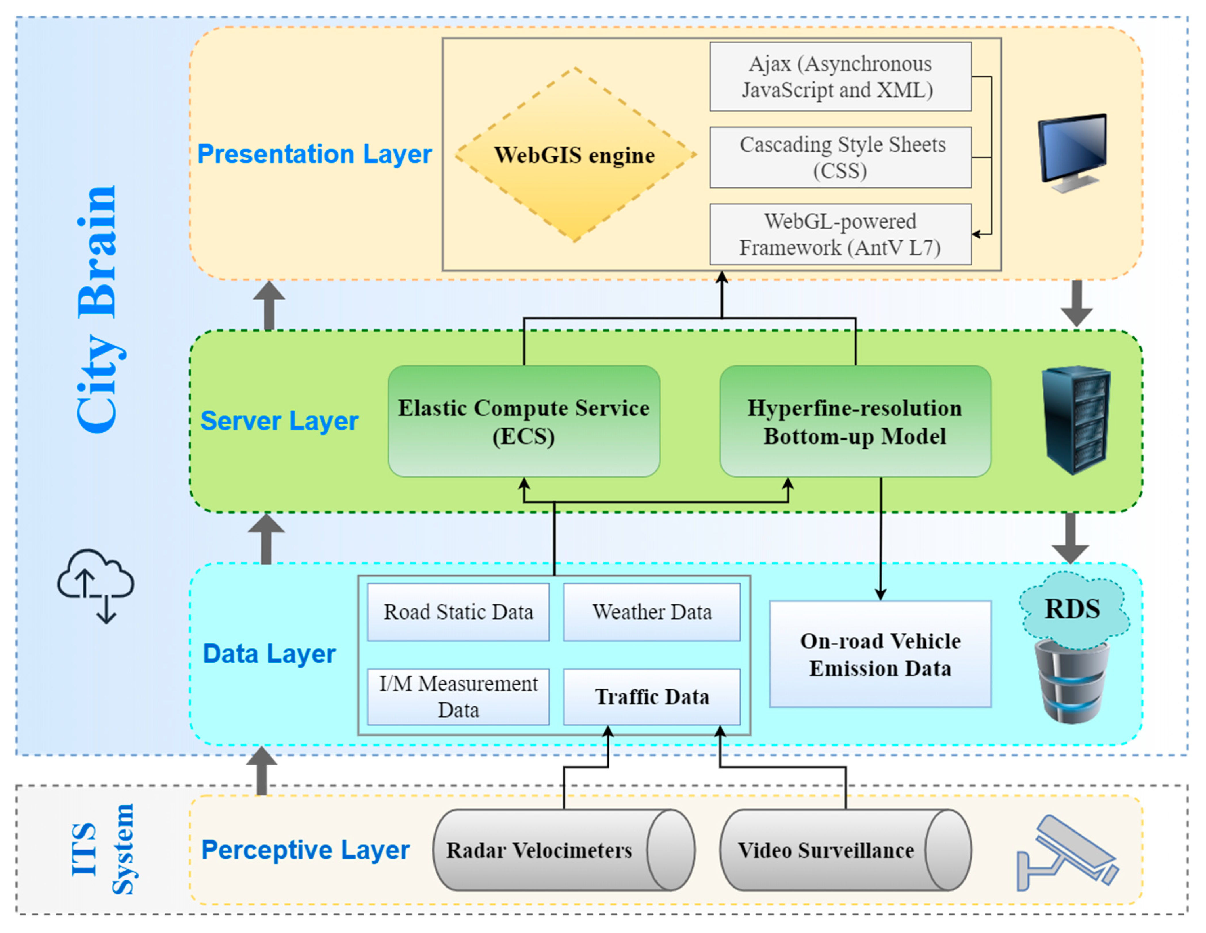
2.1. System Framework

This work aimed to develop and implement a big-data-driven intelligent modelling and visualization system for real-world, on-road vehicle emissions. As illustrated in Figure 1, we built up this system based on a classic Browser/Server (B/S) architecture [48] with four tiers, i.e., the perceptive, data, server, and presentation layers. The last three layers were erected on the “City Brain”. The first layer consisted of comprehensive traffic monitoring, which was the foundation of the whole system. After that, the data layer mainly relied on the MySQL database [49] supported by the Relational Database Service (RDS) [50] on-board the “City Brain”. Due to its high performance (e.g., large volume and high flexibility), it took responsibility for the storage and transmission of the big spatiotemporal data, including both the input and output data from other layers. On this basis, the server layer implemented an ITS that could interconnect and operate diverse traffic data from incompatible sources. A hyperfine model for on-road vehicle emissions served as the core of this system. This layer also received the user requests to invoke the information in the data layer, accessed the WebGIS application in the presentation layer, and performed corresponding feedbacks. The WebGIS engine can assemble the comprehensive spatiotemporal data analysis when the server receives user requests. In addition, the Elastic Compute Service (ECS) [51] onboard the “City Brain” accounted for basic operations, such as spatiotemporal data analyses, data sharing, and permission settings.
Between the server and presentation layers, the Ajax (Asynchronous JavaScript and XML) technology made asynchronous HTTP requests without reloading client applications [52]. Moreover, cascading style sheets (CSS) technologies were applied to improve user experiences, such as optimizing the interface layout and increasing the response speed [53]. Considering the big data feature of this system, we applied an agile WebGL-powered framework (AntV L7) [54] for large-scale geospatial data visualization and rendering. Hence, the presentation interface can display GIS applications through the B/S architecture and share spatial information resources, thus breaking the limitations of traditional operational methods.
Consequently, this system can map real-time or historical vehicle-specific emissions (i.e., PM2.5, NOx, HC, and CO) and associated traffic states (i.e., traffic fluxes, vehicle-specific images, categories, and speed) from the perspective of spatial (e.g., road links) and temporal (e.g., hourly) dimensions. On this basis, they can be zoomed in and visualized via button selection. Furthermore, the spatiotemporal analysis, such as the top five roads (e.g., in terms of on-road vehicle emissions), was also highlighted. More importantly, relying on this HPC framework, we could virtually investigate and visualize the consequences of traffic control strategies over the custom spatiotemporal scopes.

2.2. Real-World Data Collection

The Xiaoshan District is situated in Hangzhou, Zhejiang Province, China (Figure 2). From its GDP (i.e., CNY 200 billion) perspective, it ranked fifth among districts in Hangzhou in 2019. Within its limited geographical extent (i.e., 1417.8 km2), there was roughly 1953.7 km of road networks. In this context, the Xiaoshan District emerged as a vital urban transportation hub in Zhejiang Province. This indicates that air quality in urban microenvironment is significantly affected by fine-scale, on-road vehicle emissions.
It should be highlighted that all-around traffic monitoring allowed us to collect vehicle-specific data (Figure 2). Specifically, video surveillance and radar velocimeters measure vehicle-specific images and speed, respectively. First, in theory, traffic fluxes and vehicle-specific categories significantly affect the on-road vehicle emission [26,31]. In particular, traffic congestion and high-duty vehicles generally result in emission hotspots. To this end, all-around traffic video surveillances were applied to enable vehicle-specific identifications. From 1 January to 31 December 2021, we established an extensive database of more than 2400 million records. Vehicle-specific categories, licence plates, and fluxes could be identified via intelligent techniques (e.g., image recognition). We defined six vehicle categories, including HDTs (heavy-duty trucks), MDTs (middle-duty trucks), LDTs (light-duty trucks), HDVs (heavy-duty vehicles), MDVs (middle-duty vehicles), and LDVs (light-duty vehicles). It should be noted that these monitoring data were obtained from distinct video facilities, and thus were mutually incompatible. They were further required to be fused spatially and temporally. Detailed information is described in Section 2.3.
Another key driver is vehicle-specific speed, which is of great significance for arranging on-road vehicle emission factors [26]. Along with traffic video surveillance, radar velocimeters were utilized to measure vehicle-specific speed concurrently. All these data were updated in a timely manner (i.e., hourly) and stored in the historical database. Moreover, the vehicle-specific emission factors and road information were relatively static without being updated in real-time. The former was obtained from the vehicle I/M (vehicle Inspect/Maintenance) dataset in the Xiaoshan district [55]. The latter came from the Gaode Map, divided into 1393 road segments (Figure 2). The spatial resolutions were inconsistent (i.e., 10~1000 m) across road segments, adaptive to the gaps between sets of traffic monitoring. On this basis, all these road links were grouped into three types: residential streets, arterial roads, and highways. Collectively, we achieved a hyperfine map of comprehensive traffic states over the Xiaoshan District, involving vehicle-specific images, speeds, and categories, traffic fluxes, and road segments.

2.3. Real-Time Data Fusion

Comprehensive traffic states, including vehicle-specific categories, speeds, emission factors, and road segments, should be interconnected spatiotemporally (Figure 3). Generally, the standardized data quality controls were completed on respective devices in advance. Yet, vehicle-specific records came from various devices, the links between which should be identified. First, on-road video surveillance offered vehicle-specific images, including vehicle-specific license plates, categories, and fluxes. The I/M dataset would be responsible for double-checking the identification of the vehicle-specific categories according to the license plates. Subsequently, such vehicles would fall into two classes: non-registered vehicles and registered ones. Their emission factors were calculated based on the I/M dataset. Yet, the emission factors of the latter were speed-dependent and vehicle-category-specific, while those of the former were averaged based on vehicle-specific categories (Figure S1). Second, both radar velocimeters and video surveillances were in motion concurrently. We can thus apply time recorders to synchronize the monitoring for fluxes, license plates, vehicle-specific categories, and speed. Third, the static road information was independent of the real-time traffic states. Road links can serve as reliable bridges between them and interconnect vehicle-specific and road-specific information spatially and temporally. The resulting extensive database can be transferred into the subsequent bottom-up emission model and Web GIS interface. The total Data Throughput exceeds 300,000 records and 200 MB per hour.

2.4. Model Framework for On-Road Vehicle Emissions

We applied a hyperfine model framework to estimate real-world, on-road vehicle emissions (i.e., primary PM2.5, carbon monoxide (CO), hydrocarbon (HC), and nitrogen oxides (NOx)). Compared to most of the current bottom-up on-road vehicle emission model frameworks, our design was sufficiently elaborate in terms of vehicles, road, space, and time. Figure 1 presents a theoretical flow diagram of the hyperfine on-road vehicle emission model. Overall, the results relied on an ensemble estimate of vehicle-specific speeds, categories, fluxes, emission factors, and road segments [10,25,26]
E F c , j , l = t E F c , j ( v ) × T F c , h , l
E h , j , l = E F c , j , l × L l
where h and l represent the temporal (i.e., hour) and spatial (i.e., road segment) dimensions, respectively. For a given spatiotemporal dimension, E F c , j , l denotes the emission intensity of the pollutant j (g km−1 h−1).
Relying on the real-time HPC platform, our outcomes can map significant variations in the on-road vehicle emissions. On this basis, a real-time diagnosis algorithm was generated by comparing the emissions of all road links and vehicles and tracking their spatiotemporal evolution. Consequently, the road links and vehicle categories with high emissions were screened out and identified as key elements. More importantly, with the aid of the vehicle-road links, we can illustrate the contributions of different vehicle categories to different road links. This especially offered precise targets for on-road vehicle emission control strategies.

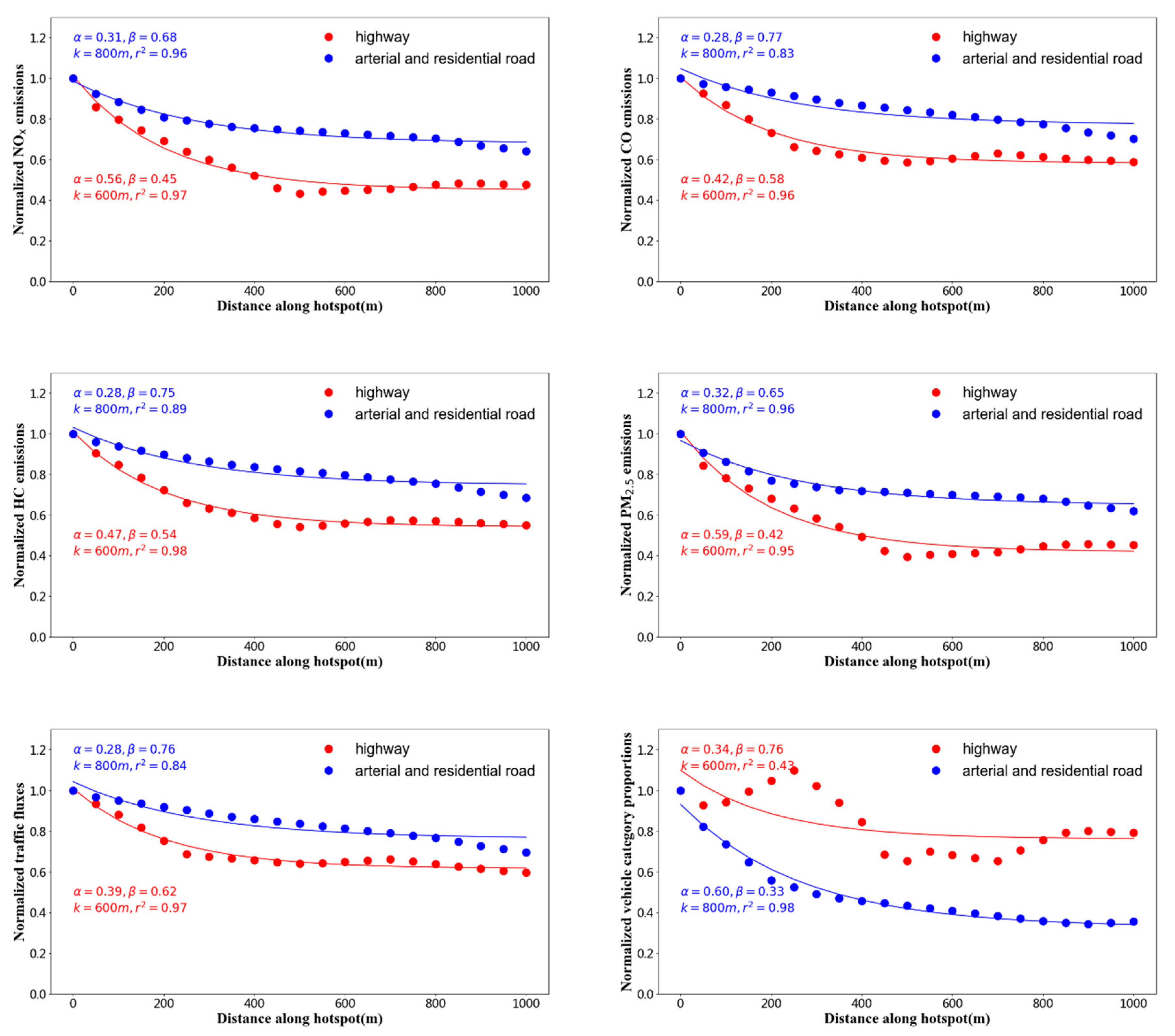
2.5. “Distance–Decay” Relationship of Hotspot Region

In theory, a comprehensive traffic profile is the basis for estimating hotspot emissions. To analyse the determinants of emission hotspot patterns, we applied an emission–distance relationship E ( d ) that might be faithfully replicated by the three-parameter unconstrained exponential model as follows:
E ( d ) = α + β exp ( 3 d / k )
where there are four parameters in this equation: the background emission ( α ); the length to the hotspot ( d , m); the slope boosted by the hotspot emissions ( β ); and the convergence coefficient ( k ), which governs the spatial scale over the emission relaxed to background emission ( α ) . In principle, the sum ( α + β ) would converge to 1.0, which suggests that the sums of the background emissions and associated increments would reflect the emission levels of the hotspots. We modelled the decay of on-road vehicle emissions, traffic fluxes, and vehicle categories from indicative hotspots outwards on annual weekdays and single hours of weekdays. Among them, annual data were used to prove the rationality of the model. Because annual and single-hour data types are homologous, we used single-hour data fitting to analyse the distance decay characteristics of real-time hotspots emission. The magnitudes of α and β reflected the amplitude of decay from hotspots at the hourly scale.

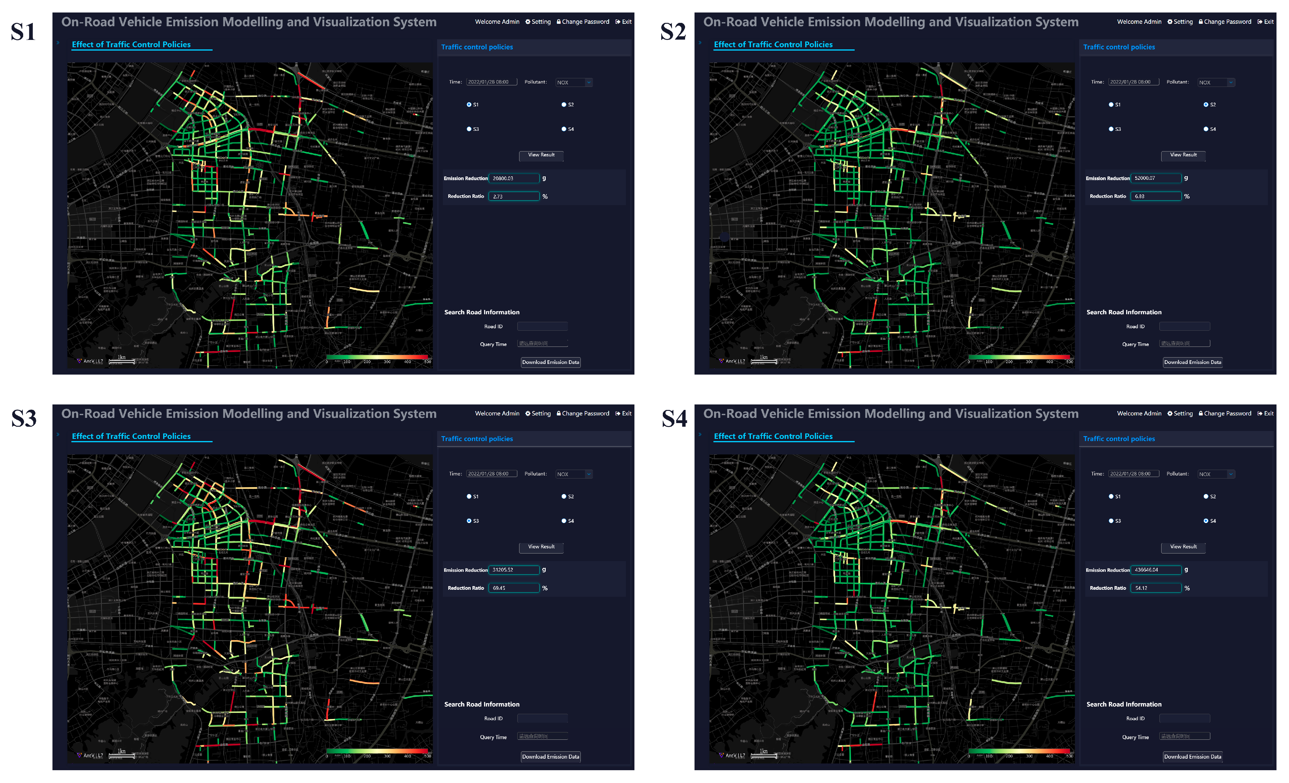
2.6. Traffic Control Strategies

Over the Xiaoshan district, routine traffic control policies were implemented to mitigate air pollution. A representative measure was on-road vehicle license restrictions, routinely operated during two typical periods, i.e., from 7:00 to 9:00 and from 16:30 to 18:30 on weekdays, so-called the morning and evening rush hours. In theory, such kinds of policies would substantially alter on-road vehicle emissions by affecting traffic states (e.g., traffic fluxes and vehicle-specific speed). Yet, the influences were still elusive.
Here we integrated the hyperfine map of on-road vehicle emissions with an agile WebGIS engine. On this basis, we can picture the impacts of traffic control measures on on-road vehicle emission reductions. We designed four traffic control scenarios with a major focus on traffic fluxes and fleet composition. The main concern was to investigate how to implement traffic control policies spatially and temporally (Table 1). Note that we virtually implemented those policies during a morning rush hour (8:00, Local time) to maximize their influences. First, the weekday scenario (S1) forbade particular vehicles according to the tail numbers of license plates. This scenario focused only on the residential and arterial roads and the morning and evening rush hours. Table 1 summarizes the detailed rules. Second, on the basis of the S1 scenario, the even–odd scenario (S2) applied the even–odd rule and thus halved traffic fluxes. This scenario was obviously more stringent than the weekday scenario (S1). Third, both non-registered and registered trucks were forbidden over the highways (S3). Fourth, we combined the S2 and S3 scenarios to achieve the strictest control on all vehicles (S4). Such a scenario was actually implemented over the Xiaoshan district during the G20 summit in 2016 [56,57,58].

3. System Application

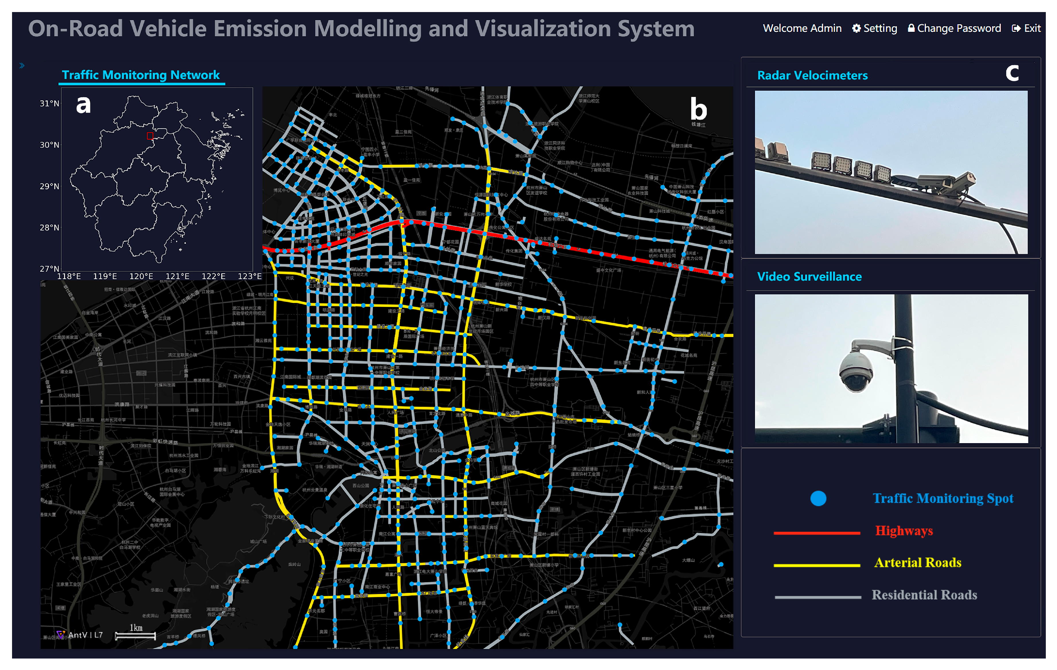
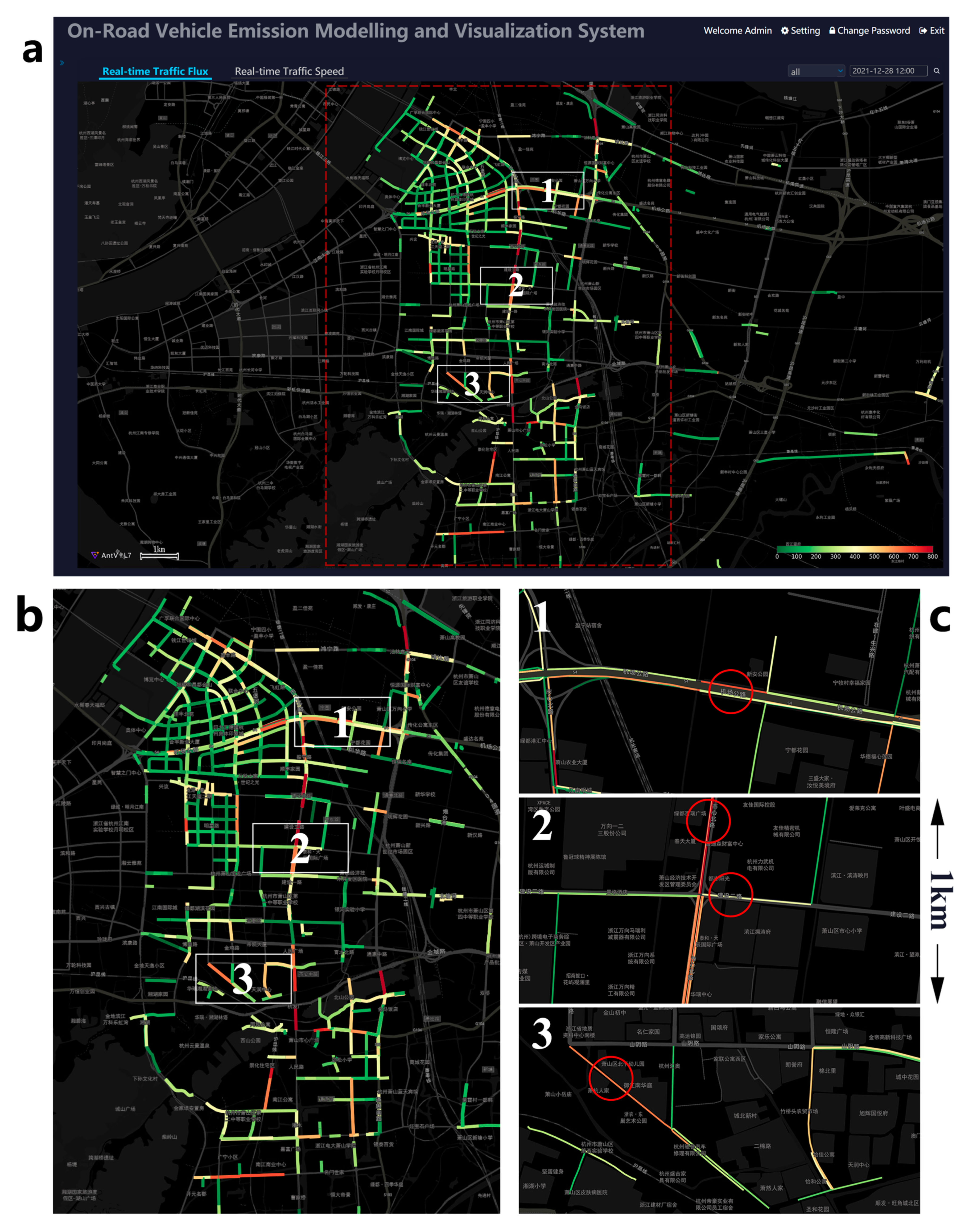
3.1. Map of Traffic Characteristics and Hotspots

This system, mainly supported by comprehensive traffic monitoring, ITS, WebGIS, and the bottom-up emission model, provided an unprecedented hyperfine map of urban traffic states in a timely manner (i.e., hourly), including vehicle-specific speed, categories, and traffic fluxes (Figure 4 and Figure 5 and Supplementary File). For instance, regarding the traffic fluxes, the colours of the links evolved from green to red, indicating a gradual increase in traffic fluxes from less than 30/h to more than 100/h. For instance, on 28 December 2021, we found that spatial distributions of traffic states were extraordinarily heterogeneous. First, as expected, the vast majority of traffic fluxes were centred on residential and arterial roads (Figure 4b). Figure 4c presents corresponding hyperfine-resolution variations in a representative 1 km2 zone. Therein, the hourly traffic flows fluctuated significantly (>25.8 times). Such large fluctuations remained even within individual streets, with an average of more than eight times. An expected finding was the frequent and widespread presence of acute geographical “traffic hotspots” across the traffic monitoring dataset. We treated individual road links or a cluster with traffic flows exceeding the district’s average level as hotspots. Through the imaging analysis coupled with all-round video surveillance, Figure 5 presents plausible drivers for some indicative hotspots. We found that traffic congestion played a key role in shaping such hotspots, which, however, were caused by a variety of factors, including high traffic volumes on key arterial or residential roads or road constructions. Further information on the technique for identifying hotspots is given in Supplementary Information.
Second, it is worth noting that, on weekdays, the daily averages of traffic fluxes were comparable to those on weekends (Figure S2). Despite this, there was a noticeable difference in hourly variation patterns between weekdays and weekends. It was clear that the morning and evening rush hours had a significant impact on the diurnal traffic fluxes on weekdays, with two maxima at 08:00 and 17:00. Our findings show that, during these periods when the traffic congestion was further exacerbated (Figure 5), the widespread hotspots were geographically stable but quantitatively more conspicuous (Figure 4d,e and Figure S3). By comparison, on weekends, there was a smaller range of traffic fluctuations, and the morning peak arrived two hours later (Figure S2). Specifically, the traffic flux peaks on weekends were roughly 80% of those on weekdays, while their hotspots were also variable, indicating more random trips (Figure S3). Therefore, the hyperfine-resolution patterns of traffic hotspots were significantly heterogeneous, and it was necessary to track them in real-time over the entire district.
Third, the spatial and temporal connections between traffic fluxes and speeds were shown to be substantial. Figure S2 presents that vehicle-specific speeds fluctuated dramatically throughout the day as a result of the varying traffic fluxes. As expected, vehicle-specific speeds were at the lowest level during the peak periods of traffic fluxes. Moreover, those peaks and valleys simultaneously shifted from weekdays to weekends. Spatially, traffic flux hotspots may have determined speed hotspots (Figure S4). Vehicle categories, on the other hand, were unaffected by traffic fluxes. After the morning rush hour, their diurnal changes were stable in regardless of the kind of roads (Figure 4 and Figure S2). Yet the HDVs and HDTs reached their peaks in the early morning hours (i.e., from 1:00 to 5:00). Additionally, the spatial distributions of vehicle categories were especially noteworthy (Figure 4f,g and Figure S5). LDVs, MDVs, LDTs, and MDTs mainly occupied the residential streets and arterial roads, while other kinds of vehicles (i.e., HDTs and HDVs) frequently appeared over the highways. We found the spatial distributions of HDVs and HDTs, the hotspots of which scattered extensively. A unique driver can be related to their large traffic fluxes, which were confirmed via video surveillance. Therefore, the fleet composition can also affect on-road vehicle emission distributions substantially, especially on small scales.

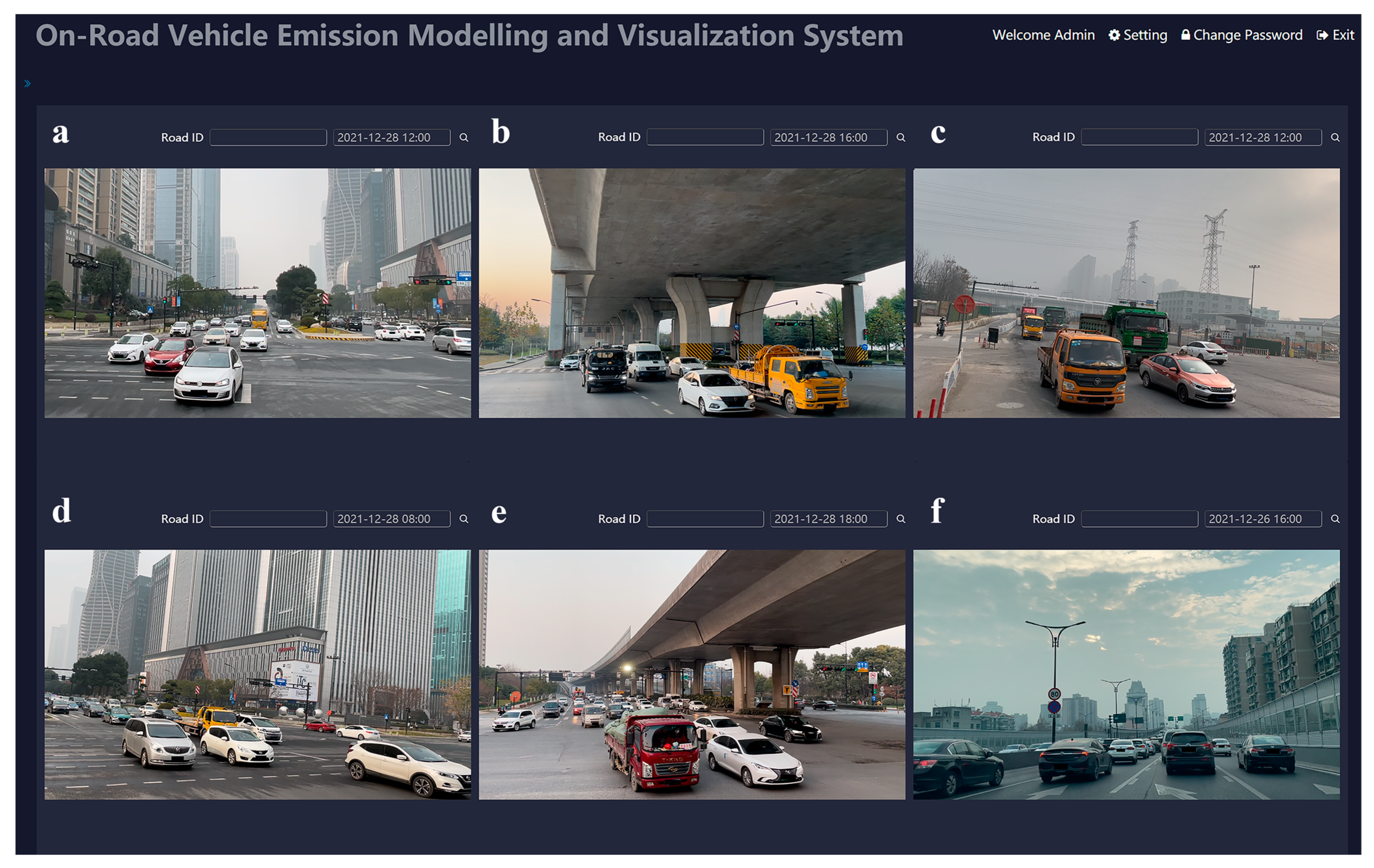
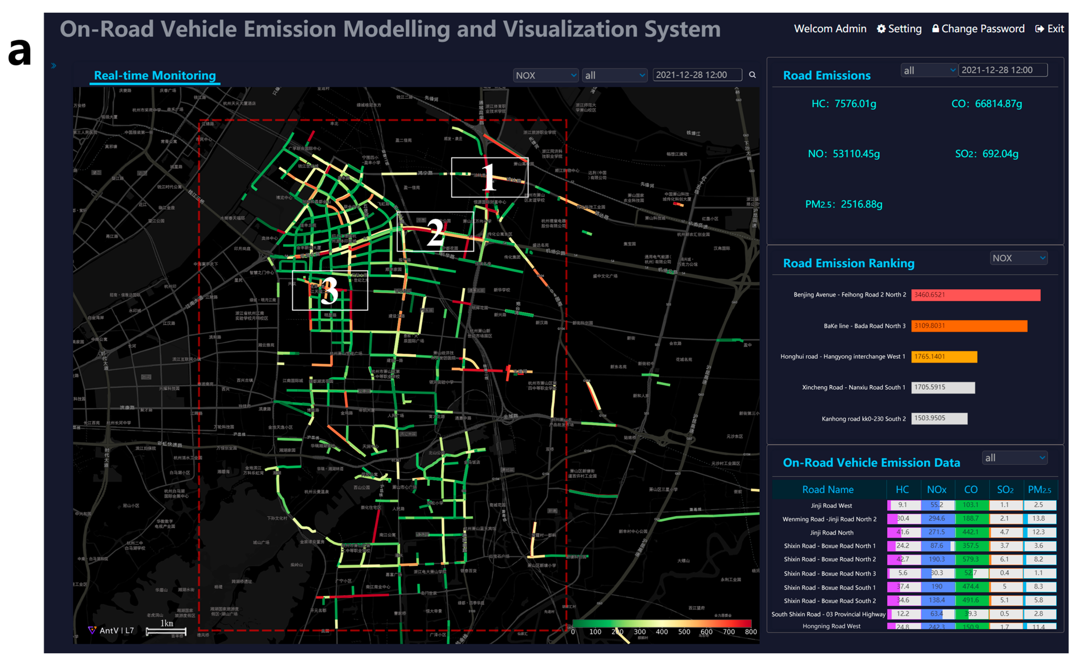
3.2. Real-Time, On-Road Vehicle Emissions

This system produced a real-time map of on-road vehicle emissions, in which widespread emission hotspots were also identified (Figure 6 and Figure S6). Such patterns were distinct from previous maps that can only capture the emissions in downtown areas, which were noticeably higher than those in suburbs. This was mostly related to the spatial distributions of vehicle categories and traffic states (Figure 5 and Figure S4). In particular, high traffic fluxes and low speeds downtown typically led to substantial on-road vehicle emissions hotspots (Figures S14 and S15). It is worth noting that towards the edge of the district, such a phenomenon was not consistent. In contrast, on-road vehicle emissions in residential streets considerably outstripped (>474.2%) those on the neighbouring roads. The spatial patterns of various vehicle categories might explain this discrepancy (Figure 4 and Figure S5). For example, emissions from HDTs and HDVs on a residential street (i.e., the Ningdong Road) contributed 86.2%, far higher than those (8.4%) in its neighbouring arterial roads (the Shixin North–Jianshe Fourth Roads).
Relying on the classified roads, Table 2 summarizes the hourly emissions of primary PM2.5, NOx, CO, and HC. The top five roads (i.e., Chenhui Road–East of Chaohui Primary School, Tonghui North Road–Hongda Road north, Airport City Avenue–Liqun River bridge west, Airport City Avenue–Minhe Road East, and Tonghui North–Hongda Road east) were also highlighted. We noted that emissions in highways, residential streets, and arterial roads increased in sequence. The primary reason for this sequence was the distinction between vehicle categories on different kinds of roads (Table S1). Taking the hourly NOx emissions (by Equation (1)) as an example, we found that they are 168.2 g/km, 102.2 g/km, and 126.7 g/km on highways, residential streets, and arterial roads, respectively. It should be noted that highways were of 3.7% of total traffic flows, while contributing 5.6% of total emissions.
Figure S7 shows that it was roughly consistent throughout the day when it came to on-road vehicle emission patterns of primary PM2.5, NOx, HC, and CO.
From the temporal perspective, it was roughly consistent throughout the day when it came to on-road vehicle emission patterns of CO, HC, NOx, and PM2.5 (Figure S7). Specifically, there was roughly 76.8% of daily NOx emissions during the daytime. In addition to this, the NOx emissions fluctuated during the daytime, but were typically stable throughout the various roads. There were, however, noticeable variations in the emissions between weekdays and weekends. As expected, the morning and evening rush hours on weekdays would also lead to peaks of on-road vehicle emissions. On the weekends, though, such trends were difficult to discern.

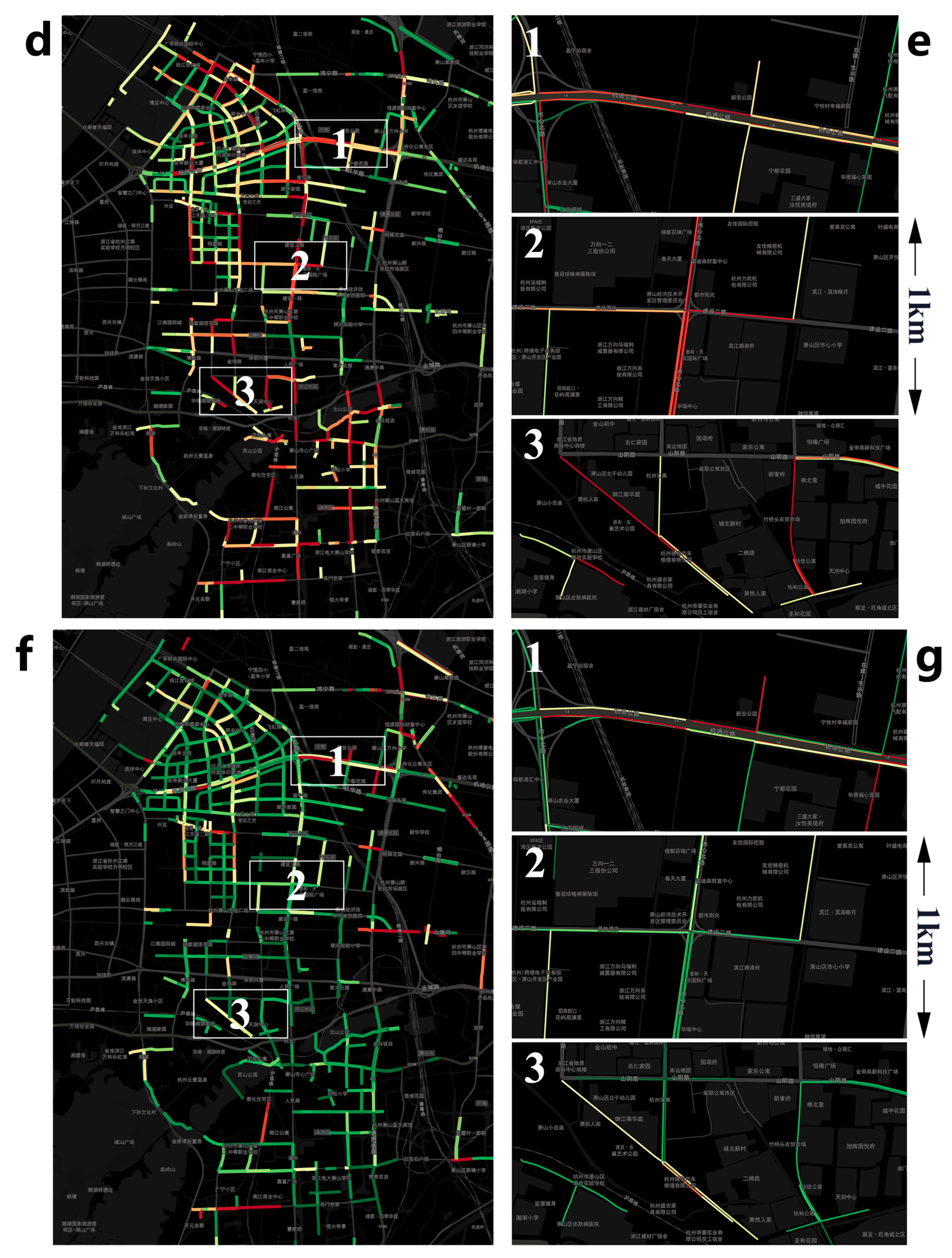
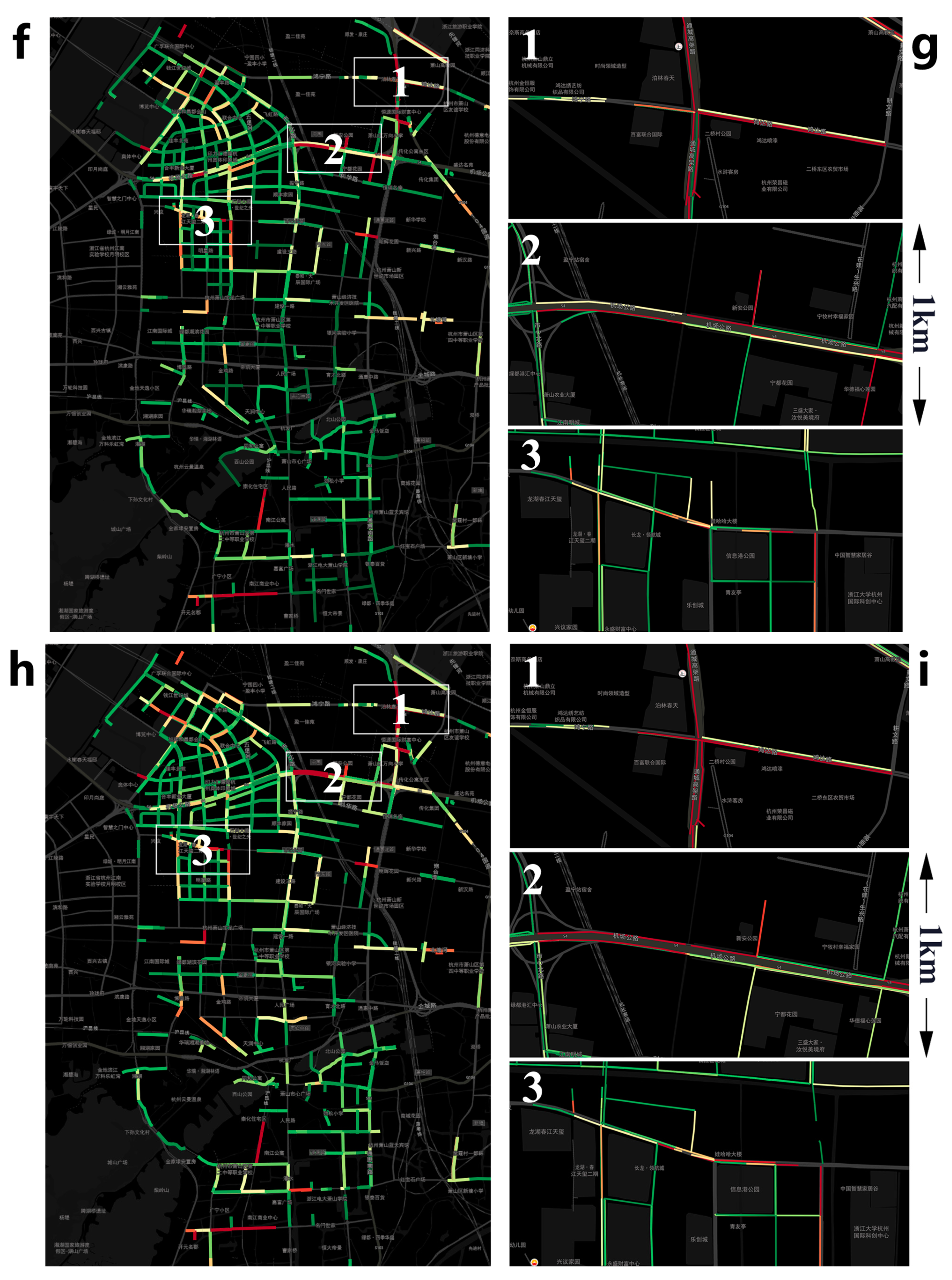
3.3. Map of Emission Hotpots and Drivers

Figure 6 depicts the hotspots of on-road vehicle emissions on major road intersections. Where two major arterial highways (North Shixin and Jiansheer Roads) intersect, the maximum of hourly average emissions appeared (Figure 4). From the spatial perspective, these emission hotspots varied significantly across various roads. For instance, hotspots in two arterial roads (i.e., the Hongda and Tonghui North Roads) emitted almost the same amount of pollutants as those in two residential streets (i.e., Jinji and Mingxing Roads), respectively (i.e., arterial roads vs. residential streets: 448.6 g/km vs. 251.1 g/km for CO; 41.3 g/km vs. 23.5 g/km for HC; 276.3 g/km vs. 161.3 g/km for NOx; and 10.6 vs. 6.2 g/km for PM2.5). However, residential streets had much lower hotspot emissions than highways and arterial roads. Specifically, hotspot emissions from the arterial roads (highways) outstripped those from residential roads by 1.8 (1.5) times for CO, 1.8 (2.1) times for HC, 1.7 (3.0) times for NOx, and 1.7 (3.2) times for primary PM2.5.
Besides, we paid particular attention to highways, in which emission hotspots were widespread and sometimes intensive (Figure 6). For instance, our emission estimates for a highway (i.e., the Airport Road) were consistently higher (1.4~2 times) than those for its neighbouring residential streets (i.e., the Yangfan Road) (Figure S8). The diurnal emission hotspots, on the other hand, were steady, geographically (Figure S9). In contrast, their emission magnitude fluctuated diurnally and between weekdays and weekends (Figure S10). As expected, the higher emission intensities generally occurred at 08:00 and 17:00.
Generally, such hotspots spanned between 100 and 200 m over the urban zones with varying emissions. Figure 7 shows that the annual hourly average emissions typically followed “distance–decay” relationships outward from the hotspot centres. The results reflected the hourly emission ratios (normalized at the hourly emissions of the hotspots) from hotspots outwards based on the distance (d). In addition, the ratios of the average traffic fluxes and vehicle category proportions were calculated in the same way. Overall, such relationships were the most sensitive for NOx and PM2.5. The annual data reflect that the locations of the hotspot areas were relatively fixed in the year. As shown in Figure 3, Figure 5 and Figure 6, we found that the traffic fluxes largely shaped the spatial emission hotspot patterns over the arterial and residential roads. Additionally, the specific vehicle category proportions (i.e., HDVs and HDTs) also played an important role.
Moreover, Figure 8 shows the decay patterns of the hourly emissions over urban zones on 28 December 2021. The results reflected a similar pattern to the average data, but we found that there existed variations in some pollutant decay patterns, indicating that road emission hotspots were not fixed consistently, and there existed spatial offsets in the short term. Meanwhile, according to the boxplot analysis of road traffic and pollutant emission data for selected hotspots in the Xiaoshan District in 2021 (Figures S12 and S13), the highway hotspot data are most consistent with the pattern. This is because there is only one highway in the Xiaoshan District, and its traffic activities have a high stability. Arterial roads and residential roads may be affected by various factors and are more sensitive to the disturbance of hotspots, but in general, they also show the corresponding pattern.
The traffic flows and emissions on highways were likewise relevant to the “distance–decay” functions, although the vehicle-specific categories kept stable therein (Figure 7). This demonstrates that traffic flows were crucial in shaping the spatial patterns of emission hotspots along the highways. Collectively, not only traffic fluxes but also specific particular vehicle categories (i.e., HDTs and HDVs) played a key role in boosting emission hotspots.

3.4. Impacts of Traffic Control Scenarios

As expected, each scenario significantly altered the traffic states spatiotemporally. The first two scenarios aimed to reduce the traffic flows, while the last two ones took into account not only traffic flows but also vehicle categories (Table 1). As a result of Table 3, the first scenario (S1) had no discernible impact on the traffic fluxes, only reducing the traffic fluxes by 3.3%. The second scenario (S2) achieved more reductions of traffic flows (8.3%). In the third scenario (S3), the fleet composition was thoroughly altered. The last scenario (S4) realized the largest reductions of the traffic flows (53.3%).
As a result of Figure 9 and Figure S11, the S1 scenario, the hourly (8:00) emission levels dropped by the modest portions (2.3% for primary PM2.5, 2.7% for NOx, 3.1% for HC, and 3.4% for CO). By comparison, more decreases were achieved over the urban zones (i.e., the residential streets and arterial roads) (5.6% for primary PM2.5, 6.8% for NOx, 7.7% for HC, and 8.5% for CO) in the S2 scenario. In parallel, the S3 scenario reduced a significant portion (4.8~79.3%) of on-road vehicle emissions over the highways. As a consequence, the S4 scenario realized the largest emission reductions (i.e., 54.3% for primary PM2.5, 54.1% for NOx, 53.6% for HC, and 53.3% for CO). On this basis, as shown in the Figure 9 (S4), the emission hotspots mostly disappeared. It should be noted that, if such scenarios came true, additional traffic states, such as vehicle-specific speeds, would also be altered. Hence, we need to conduct more realistic studies in order to better simulate the feedback associated with traffic conditions.

4. Conclusions

This paper described a system that establishes and visualizes real-time, hyper-fine, real-world, on-road vehicle emission distributions. Our results achieved an unprecedented temporal (i.e., hourly) and spatial resolution (i.e., 10 m~1 km, one to three orders higher than ever before). A key technical prerequisite is the comprehensive interconnections between the ITS and ubiquitous traffic monitoring over the Xiaoshan District. As a result, this system reveals frequent and widespread on-road vehicle emission hotspots. Around them, significant variabilities (up to 8~15 times) are exposed and attributed to large traffic fluxes and distinctive vehicle categories. This system also allows us to simulate the benefits of traffic control policies. We confirm that the most serious traffic control policy could achieve far more than 50% of emission reductions.
In this system, the traffic states, including vehicle-specific categories and speeds, are measured in real-time. By comparison, the vehicle-specific emission factors derived from the I/M dataset are of higher uncertainties [59]. Additionally, fuel-dependent differences are not taken into account when determining the emission factors. For instance, HDVs and HDTs are presumed to run on diesel fuel, whereas other vehicle types run on gasoline. In addition, the aging impacts of vehicles were overlooked. These hypotheses are supported by earlier research [26,60]. In the future, near-road emission monitoring might be used to reduce these errors. More than this, low-cost sensors such as those on taxis and mobile phones might drastically reduce the expenses of collecting data and thus widely expand our system.
Overall, the operational application of this system could reform the study of road vehicle emissions. Once our system is linked to a full CTM, real-time, hyper-fine, real-world air quality emulations would also become possible. By combining CTM output and data from near-road air quality managements, a high resolution of air quality response to emissions becomes possible. This could help investigate the complex response of air quality to anthropogenic emissions and even address exposure misclassification. Such results may have additional sociological implications, including for future urban planning and sustainable development.

Supplementary Materials

The following supporting information can be downloaded at: https://www.mdpi.com/article/10.3390/su14095434/s1.

Author Contributions

S.Y. and P.L. conceived and designed the research. L.W. (Lu Wang), X.C., Y.X., L.J. and J.Y. performed system developments. L.W. (Lu Wang), X.C., Y.X., L.J., J.Y., T.H., L.W. (Liqiang Wang), Y.Z., M.L., Z.L., Z.S. and Y.J. conducted data analysis. W.L. and X.Z. contributed to scientific discussions. S.Y. and P.L. wrote and revised the manuscript. All authors have read and agreed to the published version of the manuscript.

Funding

This study was supported by the National Natural Science Foundation of China (No. 42175084, 21577126, and 41561144004), the Department of Science and Technology of China (No. 2018YFC0213506 and 2018YFC0213503), and the National Research Program for Key Issues in Air Pollution Control in China (No. DQGG0107). Pengfei Li was supported by the National Natural Science Foundation of China (No. 22006030), the Initiation Fund for Introducing Talents of Hebei Agricultural University (412201904), and the Hebei Youth Top Fund (BJ2020032).

Data Availability Statement

All measurements and model results are available upon request.

Conflicts of Interest

The authors declare no conflict of interest.

References

  1. Liang, X.; Zhang, S.; Wu, Y.; Xing, J.; He, X.; Zhang, K.M.; Wang, S.; Hao, J. Air quality and health benefits from fleet electrification in China. Nat. Sustain. 2019, 2, 962–971. [Google Scholar] [CrossRef]
  2. Wang, L.; Chen, X.; Zhang, Y.; Li, M.; Li, P.; Jiang, L.; Xia, Y.; Li, Z.; Li, J.; Wang, L.; et al. Switching to electric vehicles can lead to significant reductions of PM2.5 and NO2 across China. One Earth 2021, 4, 1037–1048. [Google Scholar] [CrossRef]
  3. Zhang, Q.; Zheng, Y.; Tong, D.; Shao, M.; Wang, S.; Zhang, Y.; Xu, X.; Wang, J.; He, H.; Liu, W.; et al. Drivers of Improved PM2.5 Air Quality in China from 2013 to 2017; National Academy of Sciences: Washington, DC, USA, 2019; Volume 116, pp. 24463–24469. [Google Scholar]
  4. Xue, Y.; Cao, X.; Ai, Y.; Xu, K.; Zhang, Y. Primary Air Pollutants Emissions Variation Characteristics and Future Control Strategies for Transportation Sector in Beijing, China. Sustainability 2020, 12, 4111. [Google Scholar] [CrossRef]
  5. Gao, J.; Wang, K.; Wang, Y.; Liu, S.; Zhu, C.; Hao, J.; Liu, H.; Hua, S.; Tian, H. Temporal-spatial characteristics and source apportionment of PM2.5 as well as its associated chemical species in the Beijing-Tianjin-Hebei region of China. Environ. Pollut. 2018, 233, 714–724. [Google Scholar] [CrossRef] [PubMed]
  6. Ecology, M.O.; China, E.O.T.P. China Vehicle Environmental Management Annual Report; Ministry of Ecology and Environment of the People’s Republic of China: Beijing, China, 2020.
  7. Song, C.; Wu, L.; Xie, Y.; He, J.; Chen, X.; Wang, T.; Lin, Y.; Jin, T.; Wang, A.; Liu, Y.; et al. Air pollution in China: Status and spatiotemporal variations. Environ. Pollut. 2017, 227, 334–347. [Google Scholar] [CrossRef] [PubMed]
  8. Anenberg, S.C.; Miller, J.; Minjares, R.; Du, L.; Henze, D.K.; Lacey, F.; Malley, C.S.; Emberson, L.; Franco, V.; Klimont, Z.; et al. Impacts and mitigation of excess diesel-related NOx emissions in 11 major vehicle markets. Nature 2017, 545, 467–471. [Google Scholar] [CrossRef]
  9. Ogunkunle, O.; Ahmed, N.A. Overview of Biodiesel Combustion in Mitigating the Adverse Impacts of Engine Emissions on the Sustainable Human–Environment Scenario. Sustainability 2021, 13, 5465. [Google Scholar] [CrossRef]
  10. Zhang, S.; Wu, Y.; Huang, R.; Wang, J.; Yan, H.; Zheng, Y.; Hao, J. High-resolution simulation of link-level vehicle emissions andconcentrations for air pollutants in a traffic-populated eastern Asian city. Atmos. Chem. Phys. 2016, 16, 9965–9981. [Google Scholar] [CrossRef] [Green Version]
  11. Lyu, P.; Wang, P.S.; Liu, Y.; Wang, Y. Review of the studies on emission evaluation approaches for operating vehicles. J. Traffic Transp. Eng. 2021, 8, 493–509. [Google Scholar] [CrossRef]
  12. Mangones, S.C.; Jaramillo, P.; Fischbeck, P.; Rojas, N.Y. Development of a high-resolution traffic emission model: Lessons and key insights from the case of Bogotá, Colombia. Environ. Pollut. 2019, 253, 552–559. [Google Scholar] [CrossRef]
  13. Xue, H.; Jiang, S.; Liang, B. A study on the model of traffic flow and vehicle exhaust emission. Math. Probl. Eng. 2013, 2013, 736285. [Google Scholar] [CrossRef] [Green Version]
  14. Agarwal, A.K.; Mustafi, N.N. Real-world automotive emissions: Monitoring methodologies, and control measures. Renew. Sustain. Energy Rev. 2021, 137, 110624. [Google Scholar] [CrossRef]
  15. Janssens-Maenhout, G.; Crippa, M.; Guizzardi, D.; Dentener, F.; Muntean, M.; Pouliot, G.; Keating, T.; Zhang, Q.; Kurokawa, J.; Wankmüller, R.; et al. HTAP_v2.2: A mosaic of regional and global emission grid maps for 2008 and 2010 to study hemispheric transport of air pollution. Atmos. Chem. Phys. 2015, 15, 11411–11432. [Google Scholar] [CrossRef] [Green Version]
  16. Li, M.; Zhang, Q.; Kurokawa, J.; Woo, J.; He, K.; Lu, Z.; Ohara, T.; Song, Y.; Streets, D.G.; Carmichael, G.R.; et al. MIX: A mosaic Asian anthropogenic emission inventory under the international collaboration framework of the MICS-Asia and HTAP. Atmos. Chem. Phys. 2017, 17, 935–963. [Google Scholar] [CrossRef] [Green Version]
  17. Zhang, S.; Wu, Y.; Liu, H.; Wu, X.; Zhou, Y.; Yao, Z.; Fu, L.; He, K.; Hao, J. Historical evaluation of vehicle emission control in Guangzhou based on a multi-year emission inventory. Atmos. Environ. 2013, 76, 32–42. [Google Scholar] [CrossRef]
  18. Lv, W.; Hu, Y.; Li, E.; Liu, H.; Pan, H.; Ji, S.; Hayat, T.; Alsaedi, A.; Ahmad, B. Evaluation of vehicle emission in Yunnan province from 2003 to 2015. J. Clean. Prod. 2019, 207, 814–825. [Google Scholar] [CrossRef]
  19. Gately, C.K.; Hutyra, L.R.; Peterson, S.; Sue Wing, I. Urban emissions hotspots: Quantifying vehicle congestion and air pollution using mobile phone GPS data. Environ. Pollut. 2017, 229, 496–504. [Google Scholar] [CrossRef]
  20. Gately, C.K.; Hutyra, L.R. Large Uncertainties in Urban-Scale Carbon Emissions. J. Geophys. Res. Atmos. 2017, 122, 242–260. [Google Scholar] [CrossRef]
  21. Jiang, L.; Xia, Y.; Wang, L.; Chen, X.; Ye, J.; Hou, T.; Wang, L.; Zhang, Y.; Li, M.; Li, Z.; et al. Hyperfine-resolution mapping of on-road vehicle emissions with comprehensive traffic monitoring and an intelligent transportation system. Atmos. Chem. Phys. 2021, 21, 16985–17002. [Google Scholar] [CrossRef]
  22. Jing, B.; Wu, L.; Mao, H.; Gong, S.; He, J.; Zou, C.; Song, G.; Li, X.; Wu, Z. Development of a vehicle emission inventory with high temporal–spatial resolution based on NRT traffic data and its impact on air pollution in Beijing–Part 1: Development and evaluation of vehicle emission inventory. Atmos. Chem. Phys. 2016, 16, 3161–3170. [Google Scholar] [CrossRef] [Green Version]
  23. Liu, Y.; Ma, J.; Li, L.; Lin, X.; Xu, W.; Ding, H. A high temporal-spatial vehicle emission inventory based on detailed hourly traffic data in a medium-sized city of China. Environ. Pollut. 2018, 236, 324–333. [Google Scholar] [CrossRef] [PubMed]
  24. Wen, Y.; Zhang, S.; Zhang, J.; Bao, S.; Wu, X.; Yang, D.; Wu, Y. Mapping dynamic road emissions for a megacity by using open-access traffic congestion index data. Appl. Energy 2020, 260, 114357. [Google Scholar] [CrossRef]
  25. Wu, L.; Chang, M.; Wang, X.; Hang, J.; Zhang, J.; Wu, L.; Shao, M. Development of the Real-time On-road Emission (ROE v1.0) model for street-scale air quality modeling based on dynamic traffic big data. Geosci. Model. Dev. 2020, 13, 23–40. [Google Scholar] [CrossRef] [Green Version]
  26. Yang, D.; Zhang, S.; Niu, T.; Wang, Y.; Xu, H.; Zhang, K.M.; Wu, Y. High-resolution mapping of vehicle emissions of atmospheric pollutants based on large-scale, real-world traffic datasets. Atmos. Chem. Phys. 2019, 19, 8831–8843. [Google Scholar] [CrossRef] [Green Version]
  27. Yang, W.; Yu, C.; Yuan, W.; Wu, X.; Zhang, W.; Wang, X. High-resolution vehicle emission inventory and emission control policy scenario analysis, a case in the Beijing-Tianjin-Hebei (BTH) region, China. J. Clean. Prod. 2018, 203, 530–539. [Google Scholar] [CrossRef]
  28. Liu, J.; Han, K.; Chen, X.M.; Ong, G.P. Spatial-temporal inference of urban traffic emissions based on taxi trajectories and multi-source urban data. Transp. Res. Part C Emerg. Technol. 2019, 106, 145–165. [Google Scholar] [CrossRef] [Green Version]
  29. Song, X.; Guo, R.; Xia, T.; Guo, Z.; Long, Y.; Zhang, H.; Song, X.; Ryosuke, S. Mining urban sustainable performance: Millions of GPS data reveal high-emission travel attraction in Tokyo. J. Clean. Prod. 2020, 242, 118396. [Google Scholar] [CrossRef]
  30. Xia, C.; Xiang, M.; Fang, K.; Li, Y.; Ye, Y.; Shi, Z.; Liu, J. Spatial-temporal distribution of carbon emissions by daily travel and its response to urban form: A case study of Hangzhou, China. J. Clean. Prod. 2020, 257, 120797. [Google Scholar] [CrossRef]
  31. Deng, F.; Lv, Z.; Qi, L.; Wang, X.; Shi, M.; Liu, H. A big data approach to improving the vehicle emission inventory in China. Nat. Commun. 2020, 11, 2801. [Google Scholar] [CrossRef]
  32. Beaton, S.P.; Bishop, G.A.; Zhang, Y.; Stedman, D.H.; Ashbaugh, L.L.; Lawson, D.R. On-Road Vehicle Emissions: Regulations, Costs, and Benefits. Science 1995, 268, 991–993. [Google Scholar] [CrossRef]
  33. Mcgaughey, G.R.; Desai, N.R.; Allen, D.T.; Seila, R.L.; Lonneman, W.A.; Fraser, M.P.; Harley, R.A.; Pollack, A.K.; Ivy, J.M.; Price, J.H. Analysis of motor vehicle emissions in a Houston tunnel during the Texas Air Quality Study 2000. Atmos. Environ. 2004, 38, 3363–3372. [Google Scholar] [CrossRef]
  34. Paul, J.; Malhotra, B.; Dale, S.; Qiang, M. RFID based vehicular networks for smart cities. In Proceedings of the 2013 IEEE 29th International Conference on Data Engineering Workshops (ICDEW), Brisbane, Australia, 8–12 April 2013; pp. 120–127. [Google Scholar]
  35. Song, J.; Zhao, C.; Lin, T.; Li, X.; Prishchepov, A.V. Spatio-temporal patterns of traffic-related air pollutant emissions in different urban functional zones estimated by real-time video and deep learning technique. J. Clean. Prod. 2019, 238, 117881. [Google Scholar] [CrossRef]
  36. Liu, B.; Frey, H.C. Variability in Light-Duty Gasoline Vehicle Emission Factors from Trip-Based Real-World Measurements. Environ. Sci. Technol. 2015, 49, 12525–12534. [Google Scholar] [CrossRef] [PubMed]
  37. Wu, Y.; Song, G.; Yu, L. Sensitive analysis of emission rates in MOVES for developing site-specific emission database. Transp. Res. Part D Transp. Environ. 2014, 32, 193–206. [Google Scholar] [CrossRef]
  38. Yang, Z.; Peng, J.; Wu, L.; Ma, C.; Zou, C.; Wei, N.; Zhang, Y.; Liu, Y.; Andre, M.; Li, D.; et al. Speed-guided intelligent transportation system helps achieve low-carbon and green traffic: Evidence from real-world measurements. J. Clean. Prod. 2020, 268, 122230. [Google Scholar] [CrossRef]
  39. Apte, J.S.; Messier, K.P.; Gani, S.; Brauer, M.; Kirchstetter, T.W.; Lunden, M.M.; Marshall, J.D.; Portier, C.J.; Vermeulen, R.C.H.; Hamburg, S.P. High-Resolution Air Pollution Mapping with Google Street View Cars: Exploiting Big Data. Environ. Sci. Technol. 2017, 51, 6999–7008. [Google Scholar] [CrossRef]
  40. Guo, L.; Dong, M.; Ota, K.; Li, Q.; Ye, T.; Wu, J.; Li, J. A Secure Mechanism for Big Data Collection in Large Scale Internet of Vehicle. IEEE Internet Things J. 2017, 4, 601–610. [Google Scholar] [CrossRef] [Green Version]
  41. Louhghalam, A.; Akbarian, M.; Ulm, F. Carbon management of infrastructure performance: Integrated big data analytics and pavement-vehicle-interactions. J. Clean. Prod. 2017, 142, 956–964. [Google Scholar] [CrossRef]
  42. Gately, C.K.; Hutyra, L.R.; Wing, I.S.; Brondfield, M.N. A Bottom up Approach to on-road CO2 Emissions Estimates: Improved Spatial Accuracy and Applications for Regional Planning. Environ. Sci. Technol. 2013, 47, 2423–2430. [Google Scholar] [CrossRef]
  43. Avila, A.M.; Mezić, I. Data-driven analysis and forecasting of highway traffic dynamics. Nat. Commun. 2020, 11, 1–16. [Google Scholar] [CrossRef]
  44. Zhang, S.; Niu, T.; Wu, Y.; Zhang, K.M.; Wallington, T.J.; Xie, Q.; Wu, X.; Xu, H. Fine-grained vehicle emission management using intelligent transportation system data. Environ. Pollut. 2018, 241, 1027–1037. [Google Scholar] [CrossRef] [PubMed]
  45. Ding, H.; Cai, M.; Lin, X.; Chen, T.; Li, L.; Liu, Y. RTVEMVS: Real-time modeling and visualization system for vehicle emissions on an urban road network. J. Clean. Prod. 2021, 309, 127166. [Google Scholar] [CrossRef]
  46. An, J.; Huang, Y.; Huang, C.; Wang, X.; Yan, R.; Wang, Q.; Wang, H.; Jing, S.; Zhang, Y.; Liu, Y.; et al. Emission inventory of air pollutants and chemical speciation for specific anthropogenic sources based on local measurements in the Yangtze River Delta region, China. Atmos. Chem. Phys. 2021, 21, 2003–2025. [Google Scholar] [CrossRef]
  47. Hua, X. The City Brain: Towards Real-Time Search for the Real-World. In Proceedings of the 41st International ACM SIGIR Conference on Research and Development in Information Retrieval, Ann Arbor, MI, USA, 8–12 July 2018; pp. 1343–1344. [Google Scholar]
  48. Li, Q.; Zhu, H.; He, J. An Inconsistency Free Formalization of B/S Architecture. In Proceedings of the 31st IEEE Software Engineering Workshop (SEW 2007), Columbia, MD, USA, 6–8 March 2007; pp. 75–88. [Google Scholar]
  49. Williams, H.E.; Lane, D. Web Database Applications with PHP and MySQL: Building Effective Database-Driven Web Sites; O’Reilly Media, Inc.: Sevastopol, CA, USA, 2004. [Google Scholar]
  50. Carazo, J.M.; Stelzer, E.H.K. The BioImage Database Project: Organizing Multidimensional Biological Images in an Object-Relational Database. J. Struct. Biol. 1999, 125, 97–102. [Google Scholar] [CrossRef] [PubMed]
  51. Balduzzi, M.; Zaddach, J.; Balzarotti, D.; Kirda, E.; Loureiro, S. A Security Analysis of Amazon’s Elastic Compute Cloud Service. In Proceedings of the 27th Annual ACM Symposium on Applied Computing, Trento, Italy, 26–30 March 2012; pp. 1427–1434. [Google Scholar]
  52. Bruno, E.J. Ajax: Asynchronous JavaScript and XML. Dr. Dobb’s J. 2006, 31, 32–35. [Google Scholar]
  53. Waldman, C.G.; Hagel-Sorensen, C. Dynamic Generation of Cascading Style Sheets. U.S. Patent 20,070,220,480, 20 September 2007. [Google Scholar]
  54. Hu, Z.; Zhuge, C.; Ma, W. Towards a Very Large Scale Traffic Simulator for Multi-Agent Reinforcement Learning Testbeds. arXiv 2021, arXiv:2105.13907. [Google Scholar]
  55. Wu, Y.; Wang, R.; Zhou, Y.; Lin, B.; Fu, L.; He, K.; Hao, J. On-Road Vehicle Emission Control in Beijing: Past, Present, and Future. Environ. Sci. Technol. 2011, 45, 147–153. [Google Scholar] [CrossRef]
  56. Ji, Y.; Qin, X.; Wang, B.; Xu, J.; Shen, J.; Chen, J.; Huang, K.; Deng, C.; Yan, R.; Xu, K.; et al. Counteractive effects of regional transport and emission control on the formation of fine particles: A case study during the Hangzhou G20 summit. Atmos. Chem. Phys. 2018, 18, 13581–13600. [Google Scholar] [CrossRef] [Green Version]
  57. Wang, L.; Yu, S.; Li, P.; Chen, X.; Li, Z.; Zhang, Y.; Li, M.; Mehmood, K.; Liu, W.; Chai, T.; et al. Significant wintertime PM2.5 mitigation in the Yangtze River Delta, China, from 2016 to 2019: Observational constraints on anthropogenic emission controls. Atmos. Chem. Phys. 2020, 20, 14787–14800. [Google Scholar] [CrossRef]
  58. Zhang, G.; Xu, H.; Wang, H.; Xue, L.; He, J.; Xu, W.; Qi, B.; Du, R.; Liu, C.; Li, Z.; et al. Exploring the inconsistent variations in atmospheric primary and secondary pollutants during the 2016 G20 summit in Hangzhou, China: Implications from observations and models. Atmos. Chem. Phys. 2020, 20, 5391–5403. [Google Scholar] [CrossRef]
  59. Seo, J.; Park, J.; Park, J.; Park, S. Emission factor development for light-duty vehicles based on real-world emissions using emission map-based simulation. Environ. Pollut. 2021, 270, 116081. [Google Scholar] [CrossRef] [PubMed]
  60. Zhou, Y.; Zhao, Y.; Mao, P.; Zhang, Q.; Zhang, J.; Qiu, L.; Yang, Y. Development of a high-resolution emission inventory and its evaluation and application through air quality modeling for Jiangsu Province, China. Atmos. Chem. Phys. 2017, 17, 211–233. [Google Scholar] [CrossRef] [Green Version]
Figure 1. The framework of the big-data-driven intelligent modelling and visualization system for real-world, on-road vehicle emissions. This system based is on a classic Browser/Server (B/S) architecture with four tiers, i.e., the perceptive layer, data layer, server layer, and presentation layer. The last three layers were erected on the “City Brain”.
Sustainability 14 05434 g001
Figure 2. All-around traffic monitoring network. (a) The location of the Xiaoshan District in China. (b) Spatial distributions of traffic monitoring sites (dot). Correspondingly, all road links are divided into three types, including residential streets, arterial roads, and highways. (c) Each site includes radar velocimeters and surveillance cameras. Map data © 2021, AntV L7.
Sustainability 14 05434 g002
Figure 3. Data fusion. Vehicle-specific records come from diverse devices, the links between which are highlighted.
Sustainability 14 05434 g003
Figure 4. A hyperfine map of traffic fluxes via all-around traffic monitoring on 28 December 2021. (a) The whole map is first pictured. (b) Hourly (12:00, Local Time) traffic fluxes over the Xiaoshan district and (c) three indicative urban zones. The rest subgraphs are similar, but (d,e) and (f,g) are for the morning (8:00) rush hour and the hourly traffic fluxes of HDVs and HDTs, respectively. Red circles refer to traffic hotspots in Airport Road, Shixin North Road, Jiansheer Road, and Xiaohang Road. Map data © 2021, AntV L7.
Sustainability 14 05434 g004aSustainability 14 05434 g004b
Figure 5. Imagery analyses for illustrative traffic hotspots. The hotspot locations are presented in Figure 3. The common drivers of traffic hotspots are (a,b) heavy traffic fluxes, (c) road constructions, (d,e) morning and afternoon traffic rushes, and (f) heavy traffic fluxes of LDVs and MDVs.
Sustainability 14 05434 g005
Figure 6. Real-time, on-road vehicle emissions on 28 December 2021. (a) The whole system map is first pictured. (b) Hourly (12:00, Local time) on-road vehicle NOx emissions over the whole district and (c) three indicative urban zones. The rest subgraphs are similar, but (d,e), (f,g), and (h,i) are for the morning (8:00) rush hour, the emissions of HDTs and HDVs on local time (12:00), and the morning (8:00) rush hours of HDTs and HDVs, respectively. “Road Emission Ranking” displays the five highest road links of specific pollutants in road emissions, and “On-road Vehicle Emission Data” is the specific emission information of each road link. Map data © 2021, AntV L7.
Sustainability 14 05434 g006aSustainability 14 05434 g006bSustainability 14 05434 g006c
Figure 7. Relationships between the distance to the hotspot cores and normalized values in annual hotspot data. Each dot refers to the annual hourly average emission ratio (normalized to the hourly average emissions of the hotspots).
Sustainability 14 05434 g007
Figure 8. Relationships between the distance to the hotspot cores and normalized values. Each dot refers to the hourly emission ratio (normalized to the hourly emissions of the hotspots). We took 28 December 2021 as an example of the weekdays.
Sustainability 14 05434 g008
Figure 9. Effects of traffic control measures on on-road vehicle NOx emissions on 28 December 2021. The traffic control policies were applied during a morning rush hour (8:00, Local time) to maximize their influence. Map data © 2021, AntV L7.
Sustainability 14 05434 g009
Table 1. Traffic control policies.
ScenarioStrategyVehicle CategorySpatiotemporal Scale
S1Vehicles with particular tail numbers of license plates are forbidden. Specifically, the prohibited tail numbers were 1 and 9 on Monday, 2 and 8 on Tuesday, 3 and 7 on Wednesday, 4 and 6 on Thursday, and 5 and 0 on Friday.AllOver residential and arterial roads during morning and evening rush hours from Monday to Friday
S2Vehicles with even and odd tail numbers of license plates are alternately prohibited.AllOver residential and arterial roads during morning and evening rush hours from Monday to Friday
S3HDVs and HDTs are forbiddenHDVs and HDTsOver highways all day long
S4All vehicles follow the even–odd rule.AllOver all roads all day long
Table 2. The summary of on-road vehicle emissions on 28 December 2021.
Road TypeRoad LengthVehicle CategoryEmission (g)/Emission Intensity (g/km)
COHCNOxPM2.5
Highways11.1 kmHDVs and HDTs113.5/10.283.3/7.51300.2/116.861.1/5.5
Total2381.1/213.9247.4/22.21872.2/168.277.0/6.9
Arterial roads63.5 kmHDVs and HDTs348.7/5.5257.6/4.13988.2/62.8187.3/3.0
Total16,398.9/258.41419.1/22.48039.3/126.7299.9/4.7
Residential streets232.0 kmHDVs and HDTs1308.0/5.6978.5/4.214,891.9/64.2698.5/3.0
Total36,085.2/155.53501.2/15.123,703.0/102.2944.4/4.1
Table 3. Impacts of traffic control policies in custom spatiotemporal scopes.
ScenarioTraffic Fluxes ReductionOn-Road Vehicle Emissions Reduction
CONOHCPM2.5
S13.3%3.4%2.7%3.1%2.3%
S28.3%8.5%6.8%7.7%5.6%
S33.7%4.8%69.4%33.7%79.3%
S453.3%53.3%54.1%53.6%54.3%
Publisher’s Note: MDPI stays neutral with regard to jurisdictional claims in published maps and institutional affiliations.

