1. Introduction
Various architectural and engineering solutions, including the compaction of personal space, cannot stop urban development. For sustainable use of land area, higher buildings are being built. This causes various technical problems, such as the usage of specific lightweight structures, the guarantee of wind [
1,
2,
3] and earthquake [
4] resistance, the impact reduction of solar radiation on facades [
5,
6] of high rise buildings, the demand for shading devices [
7,
8], etc. Underground metros have already become commonplace in the cities. To save on space, parking lots, storage, and other premises are commonly constructed underground also.
Living in underground residential buildings seems like a challenge or a temporary solution. The saving of built-up area on the ground is often indicated as the main and the single advantage of underground buildings. Many disadvantages are highlighted [
9,
10]: lack of fresh air—the need for a mechanical ventilation system; darkness—the requirement of artificial lighting [
11]; the risk of obtaining rapid and safe evacuation due to landslides and flooding (especially during earthquakes) [
12]; no view through the windows; closed and limited space—claustrophobic problems; expensive construction and maintenance; expensive and complex repairs [
9]. Increased air humidity, cold, and mould are often mentioned. The issues of ventilation and light could be accepted, but the other disadvantages mentioned are the objects for discussion. Underground buildings are safer than a typical one in the event of an earthquake, and especially a tornado. In the case of an underground building, privacy is preserved, and the layout of the living space is invisible and unpredictable to outsiders. A reduced view through the window could be compensated for by noise elimination. Besides, underground buildings do not need exterior decoration.
Energy demand for the heating and cooling of a buildings’ space is a fundamental issue. Energy demand during the cold period (heating season) increases by 40% due to the need for space heating in cold climate countries [
13,
14]. Additionally, space cooling is needed in summer (non-heating season) [
15,
16]. Many methods and technologies [
17,
18,
19] have been developed to this reduce energy demand. However, the level of demand is still high to be entirely met by renewable energy sources or biofuels. Heat exchange through external partitions could be reduced by ensuring the building’s airtightness requirement, as well as thermally insulating it [
20,
21,
22,
23]. This is a traditional method to reduce energy consumption, including in new or renovated buildings.
Theoretically, the energy demand for heating or cooling the underground building must be lower than that built on the ground, because the direct impact of the wind on the heat exchange of the building to the environment is eliminated. Soil temperature is higher than the air temperature in winter and lower in summer [
24]. This aspect could be used to reduce the level of energy demand for space heating and cooling of deepened or underground buildings.
Thermal energy mainly transfers through the buildings’ external partitions to the soil by conduction, in the case of a building located above the groundwater level. Heat transfer by radiation or convection amounts only an insignificant part of the total and could be neglected [
25,
26]. The area of external surfaces, the material of the partitions and its temperatures, and the soil type, its specific heat capacity and thermal conductivity [
27,
28], and temperatures must be known to find the heat transfer intensity to the soil. These parameters and their dependence on soil density and moisture are known for the most common soils, such as clay, loam, sand, or gravel [
28]. It should be noted that some simplifications are applied in the calculations: the soil is homogeneous in a layer, and the properties are the same in all directions. The issue of soil irrigation and drying is considered only as a change in the thermal properties of the soil, and it is commonly assumed that it has constant moisture for a certain period. For typical buildings with a basement, heat transfer to the ground takes place through the basement floor and walls at a depth of up to 3 m. Here, the average season soil temperature is taken into account in the calculations. The influence of depth on the soil temperature is not considered [
29].
Physical processes near the ground surface are complex. During the sunlight period of the day, the ground surface is exposed by solar radiation. This depends on the cloudiness and the transparency of the atmosphere. Absorbed solar thermal energy spreads to the deeper layers. The top layers of the soil also radiate a part of the energy back to the atmosphere. A significant influence of daily air temperature on the soil temperature is observable up to a depth of 0.5 m and slightly smaller up to a depth of 1 m [
26,
30,
31]. It was noticed that the influence of the daily air temperature on deeper soil layers is already insignificant [
26,
31]. The process of absorption of rainwater into the ground and the impact of the rain on the soil thermal properties have not been investigated enough.
The change in soil temperature at different depths during the year has become an object of scientific research [
32,
33,
34]. The average monthly air temperature and seasonality affect the temperature of deeper (more than 1 m) soil layers. The geographical place and altitude influence soil temperature also. It has been noticed that the soil temperature remains almost constant at a depth of more than 10 m. A numerical model was performed for the soil temperature distribution by its depth in London and two cities in Egypt [
24,
35]. Simulations were based on data from the experimental investigation in Guildford, Surrey [
24]. Although it was stated that a relatively constant temperature would allow the sustainable usage of heat for efficient heating and cooling building, the proposed depth is quite considerable, being more than 10 m [
24]. The groundwater affects the thermal properties of the soil and temperature profile. Groundwater usually results in a more abrupt transition to lower temperatures and almost steady temperatures starting from lesser depths [
24]. However, it has an insignificant impact on the temperature profile of the soils of low permeability, such as clay [
24].
Heat loss to the ground needs to be evaluated accurately to reach the highest efficiency of the heating and cooling systems of the building. Different investigations have been performed [
36,
37,
38] in this field. However, simplified methodologies for calculations have been used until now [
29]. The main focus of this research was directed at structural calculations. This research aimed to determine the energy demand for the underground buildings and compare that with the case of the typical ones.
Heat transfer through building partitions acts on the increase in the temperature of the soil. However, heat spreads further and dissipates in the surrounding soil medium. After a time interval, a dynamic equilibrium is reached. Heat loss to the soil could also be treated as the charge of the soil by heat. This phenomenon was researched, focusing on the processes of charging and heat dissipation in the soil.
The task of the research presented in this paper was to reduce significantly the demand for energy for building heating or cooling by constructing it underground and exploiting the difference in temperature between soil and ambient air. The development of the sustainable usage of natural resources in the sector of civil engineering is expected to contribute to the mitigation of climate change.
2. Materials and Methods
The heat transferred to the ground through the partitions of the building could be treated as the charge of the soil by heat. Increased ground temperature means the change in the conditions of the heat transfer acting against the heat loss. The ability of the soil to retain the heat for a longer period would mean lower heat loss and energy demand for the building’s heating.
The soil-charging process was investigated in the laboratory. Thermal accumulation properties of the ground were researched in field conditions. Computation of the energy demand for the heating of the building was performed by numerical simulation.
2.1. Laboratory Experimental Setup
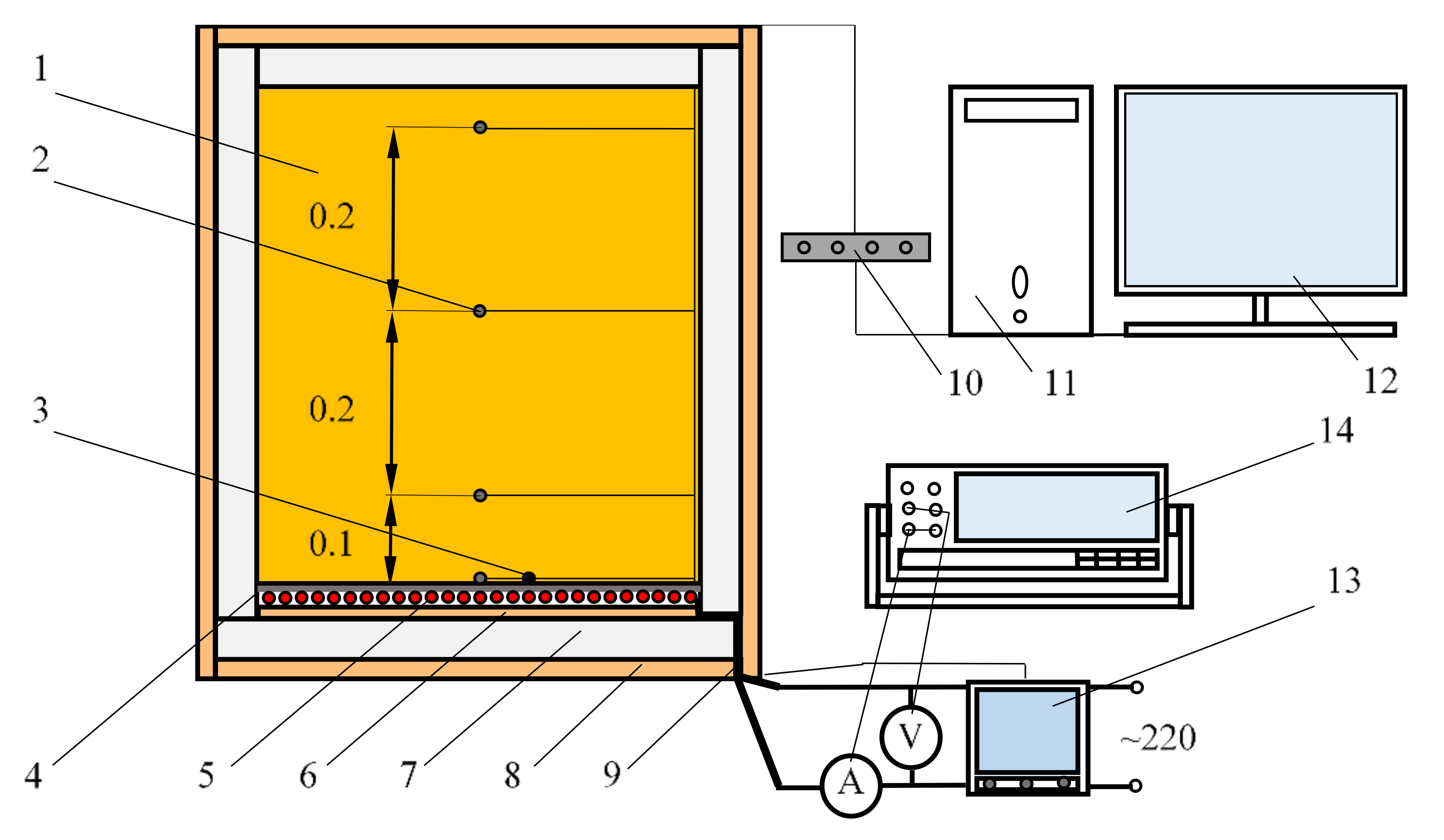
A heating cable CTAV-18, 24 m, 420 W was used for electrical heating. It was evenly routed onto the surface of the plane board as shown in
Figure 1. The length
L, width
W and the thickness
δ of it were accordingly equal to:
L =
W = 0.50 m and
δ = 0.01 m. A flat steel plate (
L =
W = 0.50 m and
δ = 0.001 m) was placed on the cable to distribute heat evenly. The outer part of the steel plate represented the heating surface during the experimental research. Heating equipment was composed of the mentioned parts. Two identical heating devices were made. One of them was installed into the laboratory setup, other was used for the experiments in field conditions. In the first case, the heating device was installed at the bottom of the box, which was internally thermal-insulated by expanded polystyrene EPS70 (
δ = 0.05 m) as shown in
Figure 1. The internal volume of the box was 0.15 m
3 (
L =
W = 0.50 m and the height equal to:
h = 0.6 m). A soil sample (sand) was placed here.
Thermal properties of the soil could be defined by type, density ρ, humidity µ, thermal conductivity λs, and specific heat cp. The sand (0/4) parameters were accordingly equal to: ρ = 1800 kg/m3, µ = 10%, λs = 1.45 W/(m·K), cp = 840 J/(kg·K).
Soil temperature was measured by platinum resistance thermometers Pt1000 (precision class A). The first sensor was placed at the center of the heated surface, the second at 0.10 m height, the third at 0.30 m, and the fourth at the height equal to 0.50 m (
Figure 2). The electric resistances of the thermometers were read and transferred to the computer by the data storage device Data Logger PT–104.
The temperature of the heated surface was set and kept by the temperature controller ATR244-12ABC or manually. An NTC type temperature sensor was additionally installed at the heated surface and used as the input signal for the controller. Voltage was measured at the connections of the heating cable by multimeter “ESCORT 3136A”. The second input channel of this device was used for electric current measurement. During the experiments, the power of the heating device was equal to P = 420 ± 10 W.
2.2. Experimental Setup for Research in Field Conditions
To perform the experimental study in the field conditions, a heating device was placed in the soil (clay) at 1 m depth. Clay density ρ, humidity µ, thermal conductivity λs, and specific heat capacity cp were accordingly equal to: ρ = 1460 kg/m3, µ = 15%, λs = 0.76 W/(m·K), cp = 878 J/(kg·K). This allowed researching the accumulation of heat in the soil under adverse conditions by the impact of the atmosphere air temperature. It was necessary to avoid the influence of the groundwater on the results at the same time. There, the groundwater surface was at a level a bit deeper than 2 m.
The heating surface was oriented downwards to simulate the case of heat loss through the basement floor. Thermal insulation of 0.1 m thickness was placed from above the heating device, as shown in
Figure 3. The thermal sensors Pt1000 were placed at different depths: at the center of the heated surface, at the distance of 0.25 m and 0.5 m from it, and one more at the side of the heating surface (
Figure 3). It was an effort not to damage the integrity of the soil.
An additional four sensors, Pt1000, were placed on the side at more than three metres from the heating surface. The air temperature was measured at an altitude of 1.5 m, covering the thermometer from direct sunlight and precipitation. One sensor was at the ground surface, another at a depth of 0.25 m, and the third at a depth of 0.5 m (
Figure 3). Data were read and transferred to the computer by Data Logger PT-104. The multimeter ESCORT 3136A was used to measure the electric current and voltage. The process of the heating was controlled by ATR244-12ABC.
To check the reproducibility and reliability of the results of the experimental investigation, the statistical parameters were calculated for every test series and performed under the same conditions. It was determined that the results of the experimental research were quite precise, reliable, and reproducible [
39].
2.3. Conditions for Numerical Simulation
Several cases are possible when defining the position of the building in relation to the ground surface: (a) the building is on the ground, (b) part of the building is in the ground, (c) the building is underground and the horizontal roof of the building is at the ground level; (d) the building is underground. In the last case, one wall must be fully or partially exposed in order to enter the building. The wind, precipitation, solar radiation, and changes in atmospheric temperature influence the place of entry.
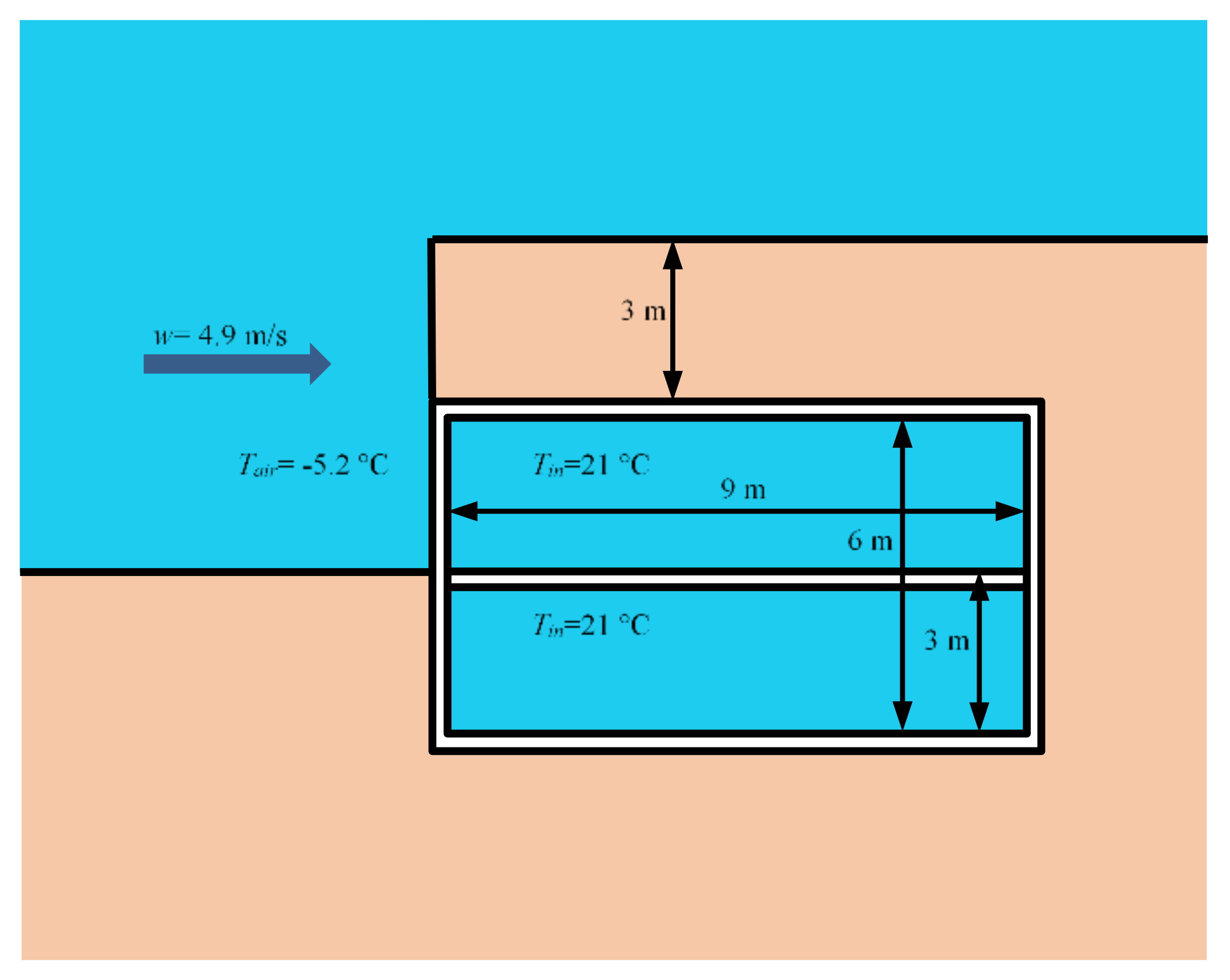
An underground building with one semi-exposed facade (
Figure 4) was selected for numerical simulation. The imaginary building had a shape of a rectangular parallelepiped. Such a shape of the building was chosen to compute the heat flux through each façade into the ground. Design and structure solutions were not considered, and analysis limited only to defining the thermal properties of the partitions. The building length
L and, width
W and the height
h were accordingly equal to
L =
W = 9 m and
h = 6 m. The thickness
δ and the value of thermal conductivity coefficient
λ of external partitions were accordingly equal to
δ = 0.3 m and
λ = 0.04 W/(m·K). The air temperature inside the building was set constant and equal to:
Tin = 21 °C [
29].
The environmental conditions and the dependence of ground temperature on the depth (
Table 1) were defined according to the meteorological parameters in Lithuania (near Kaunas town) [
40]. Average monthly temperature
Tair and wind speed
w in January:
Tair = −5.2 °C and
w = 4.9 m/s, in July:
Tair = 16.2 °C and
w = 3.1 m/s, in October:
Tair = 7.1 °C and
w = 4.9 m/s and in April:
Tair = 5.8 °C and
w = 4.9 m/s. The facade of the entrance of the building was directed to the south. It meant that it was against the wind’s predominant direction in January.
Thermal properties of the soil could be defined by type, density ρ, humidity µ, thermal conductivity λs, and specific heat cp. The sand was selected for numerical simulation, for which parameters were accordingly equal to: ρ = 1607 kg/m3, µ = 15%, λs = 1.45 W/(m·K), cp = 840 J/(kg·K). It was assumed that heat dissipated in the soil only by conduction.
Numerical simulation was based on the finite element method using Ansys software.
3. Results
3.1. Experimental Research in Laboratory
The experimental research was performed to investigate the process of thermal charging, the inertia of heat dissipation in the soil, and the accumulation properties of the soil. The experiment was started from the initial temperature of the soil sample equal to
Tstart ≈ 23.2 °C. The same temperature was of the ambient air in the laboratory. The temperature controller was set to keep the temperature of the heated surface at
Tset = 40 °C in order to start from higher difference in temperatures (Δ
T ≥ 15 K, here Δ
T =
Tset −
T0) and to have a more intensive process. The change in temperature of the heated soil sample during the first 24 h is shown in
Figure 5.
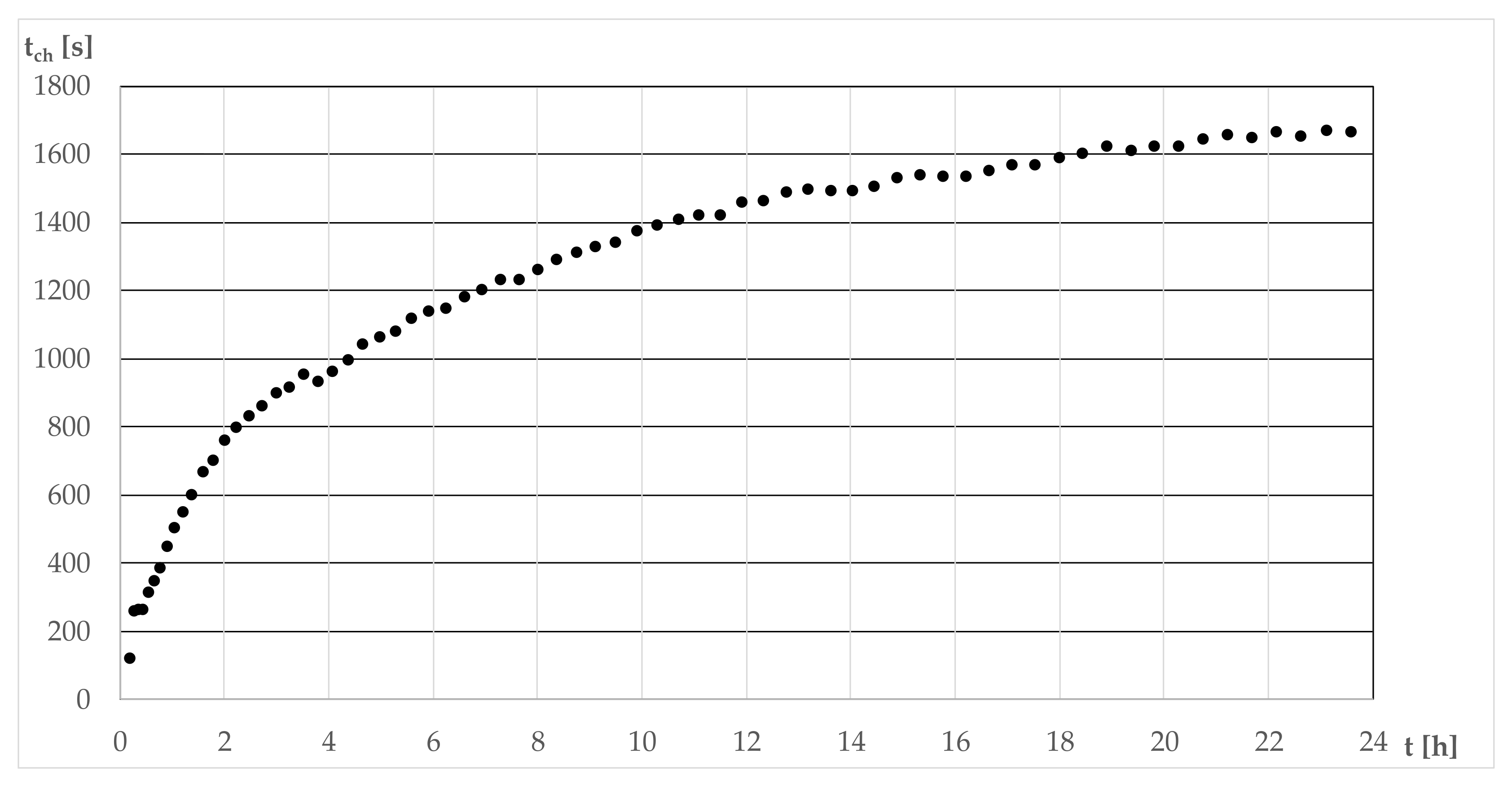
The controller turned on the heating device at the beginning of the experiment. It was switched off at the moment of the reached set temperature (T0m = Tset = 40 °C). A working heating device meant the heating cable was connected to electricity and it was called the charge. The main reason for charging up to a fixed set temperature was the prevention of the equipment overheating. This is important in practice.
The first charge lasted 310 s, the second 53 s, and the third 48 s. Gradually, the charging time approached a time interval equal to
t = 38 s. The disconnected heating device meant the time interval between charges increased with growing sample temperatures (
Figure 6).
Soil charging by heat was performed discretely by switching the heating device on or off. Therefore, the average charge intensity for the given time intervals was calculated. The average heat flux density (charge intensity) was computed according to the following equation:
where
qav is the average heat flux density,
tset is the time interval for which the average heat flux density was calculated,
i is the number indicating the specific charge,
n is the number of charges per set time interval,
Pi is the power of the specific charge (it calculated from electrical parameters of the heating device),
ti is the duration of a specific charge,
A is the area of the heating surface.
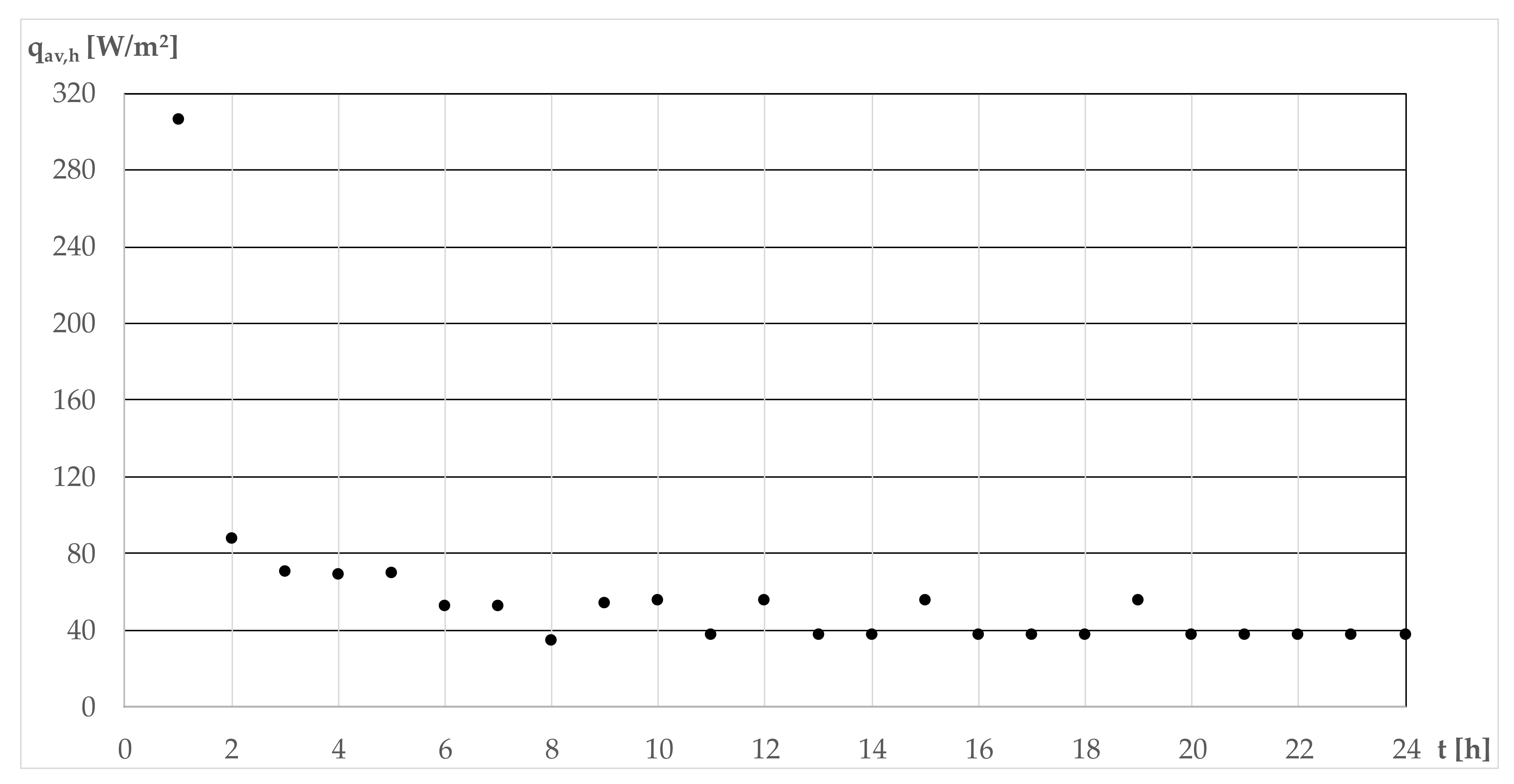
The average heat flux density of the first hour was equal to
qav,h = 306 W/m
2, of the second:
qav,h = 88 W/m
2. As the soil temperature increased, the conditions for charging the soil worsened.
qav,h decreased to an almost constant value equal to
qav,h = 37.2 W/m
2, which was reached at the eleventh hour of the first day (
Figure 7). The average heat flux density for the first day was equal to
qav,h = 59.5 W/m
2. The temperature sensor at the heating surface (0 m) showed the operation of the controller. The heat reached the thermometer placed at
h = 0.1 m (
Figure 5) after
t = 27 min.
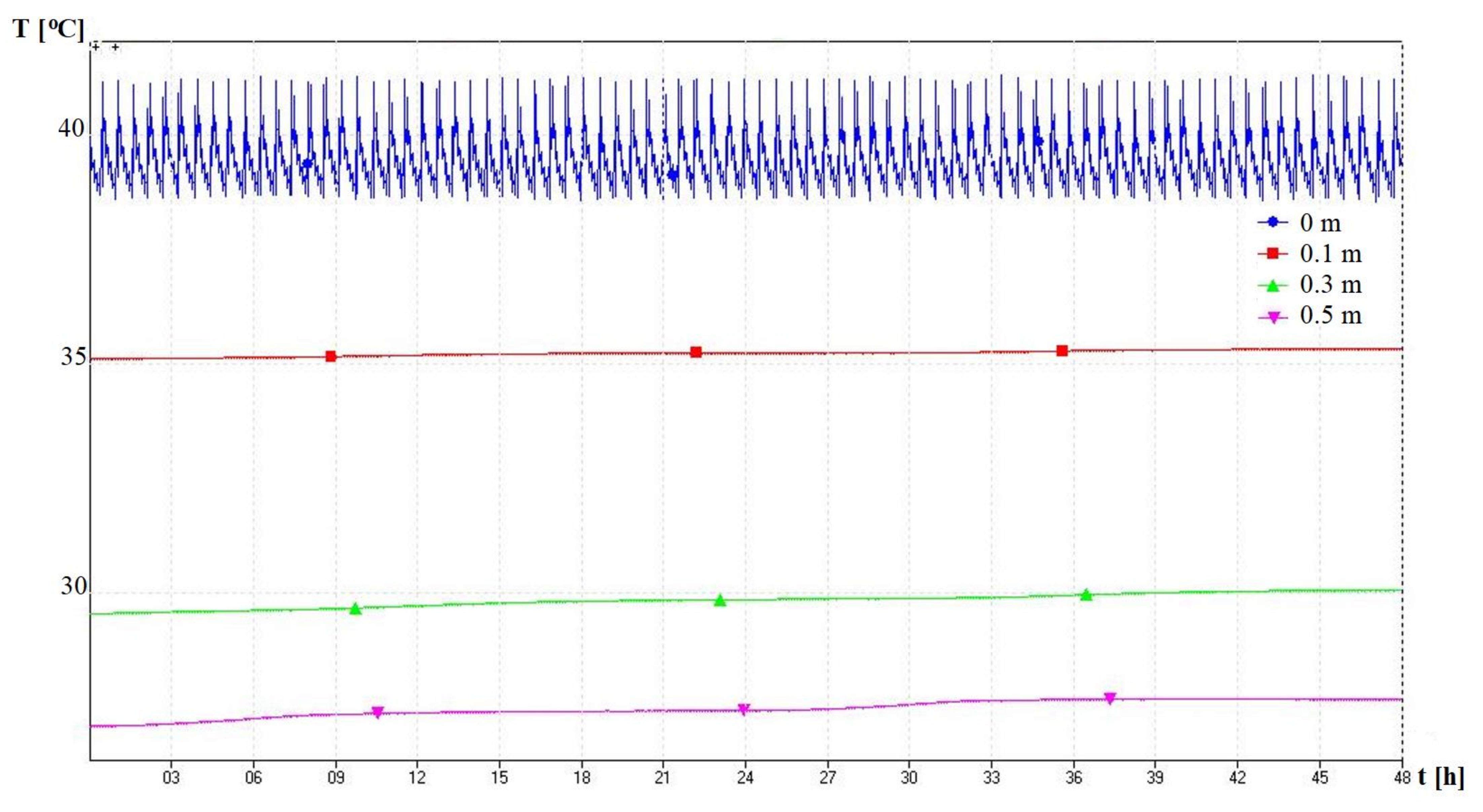
The change in temperature of the heated soil sample during the next two days is shown in
Figure 8.
During the first day, the soil temperature has changed from
T0.1m = 23.38 °C to
T0.1m = 33.36 °C at a distance
h = 0.1 m from the heating surface, from
T0.3m = 23.30 °C to
T0.3m = 25.67 °C at
h = 0.3 m, and from
T0.5m = 23.21 °C to
T0.5m = 24.07 °C at
h = 0.5 m. In the following two days, the temperature increase was equal to Δ
T0.1m = 1.53 °C, Δ
T0.3m = 2.92 °C, and Δ
T0.5m = 2.33 °C (
Figure 8). During the fifth and sixth days, the temperature increased very slightly: Δ
T0.1m = 0.21 °C, Δ
T0.3m = 0.51 °C and Δ
T0.5m = 0.59 °C (
Figure 9), and in the seventh and eighth days: Δ
T0.1m = 0.07 °C, Δ
T0.3m = 0.16 °C and Δ
T0.5m = 0.19 °C; the temperature values did not change during the ninth day.
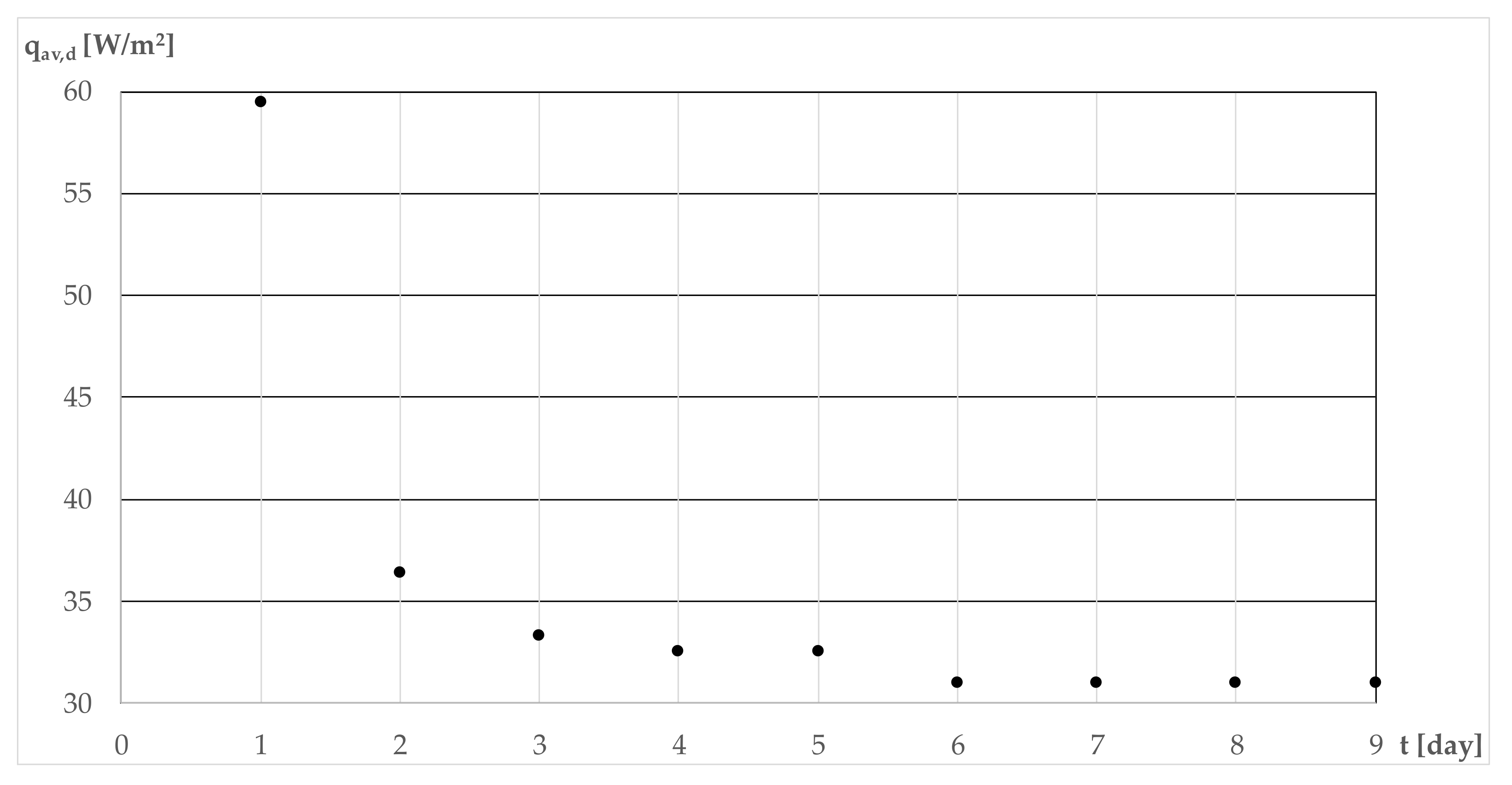
The soil was charged by heat for nine days. The average daily heat flux density was calculated (
Figure 10). Due to the maximum temperature difference between the heated surface and the adjacent soil layer, the highest charge intensity was found on the first day (
qav,d = 59.5 W/m
2) and the first hour (
Figure 7). From the sixth day, the constant value of the average heat flux density was observed:
qav,d = 31 W/m
2 (
Table 2).
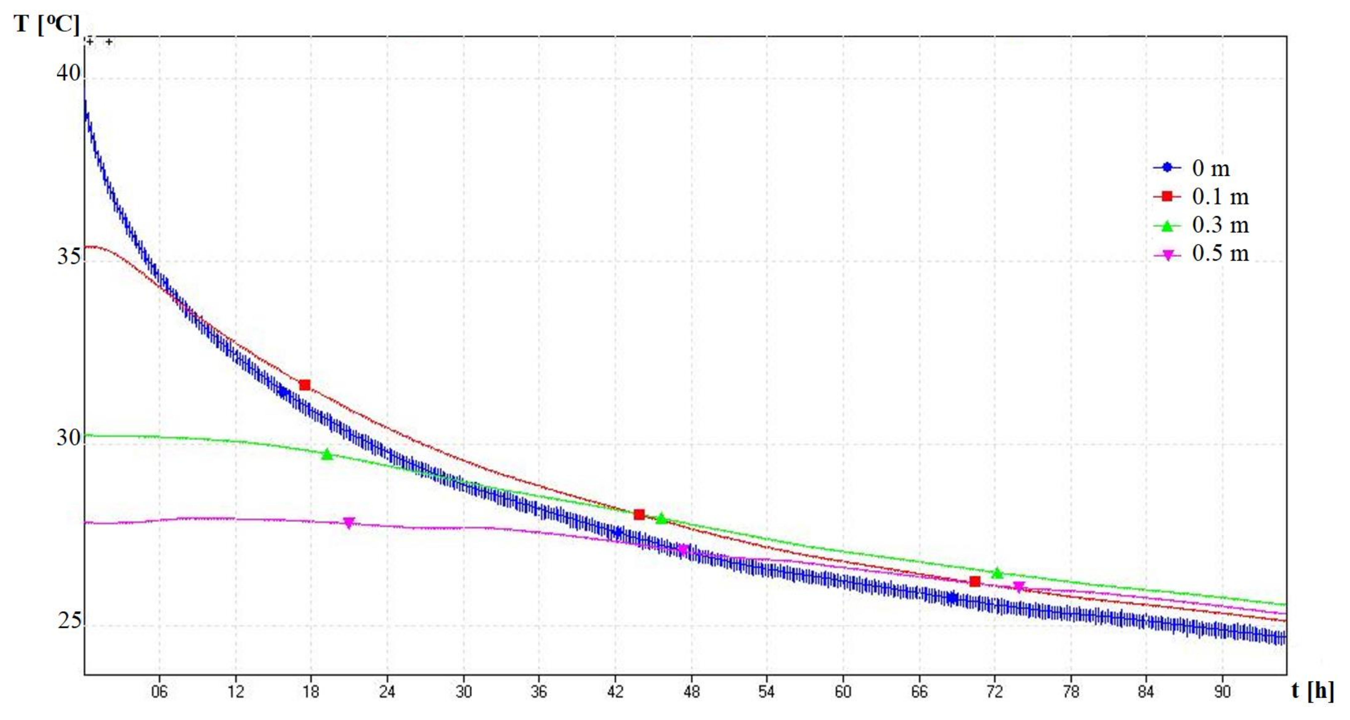
After nine days, the heating device was turned off, but the experimental research was continued for another four days, by measuring the temperatures and observing the heat dissipation in the soil. The change in temperature of the not-heated soil sample during the four days is shown in
Figure 11.
In practice, a case analogous to our research could be generated. This would require thermal insulation around the underground building to separate a certain volume of the soil. The greatest heat loss through the partitions of the underground building would be at the heating start of the unheated building. The largest temperature difference would cause the greatest heat loss. In the initial stage, there would be an intense heat charge into the soil. An increase in soil temperature would mean a decreasing temperature difference and worse conditions for heat exchange. Therefore, the heat loss would start to decrease.
3.2. Experimental Research in Field Conditions
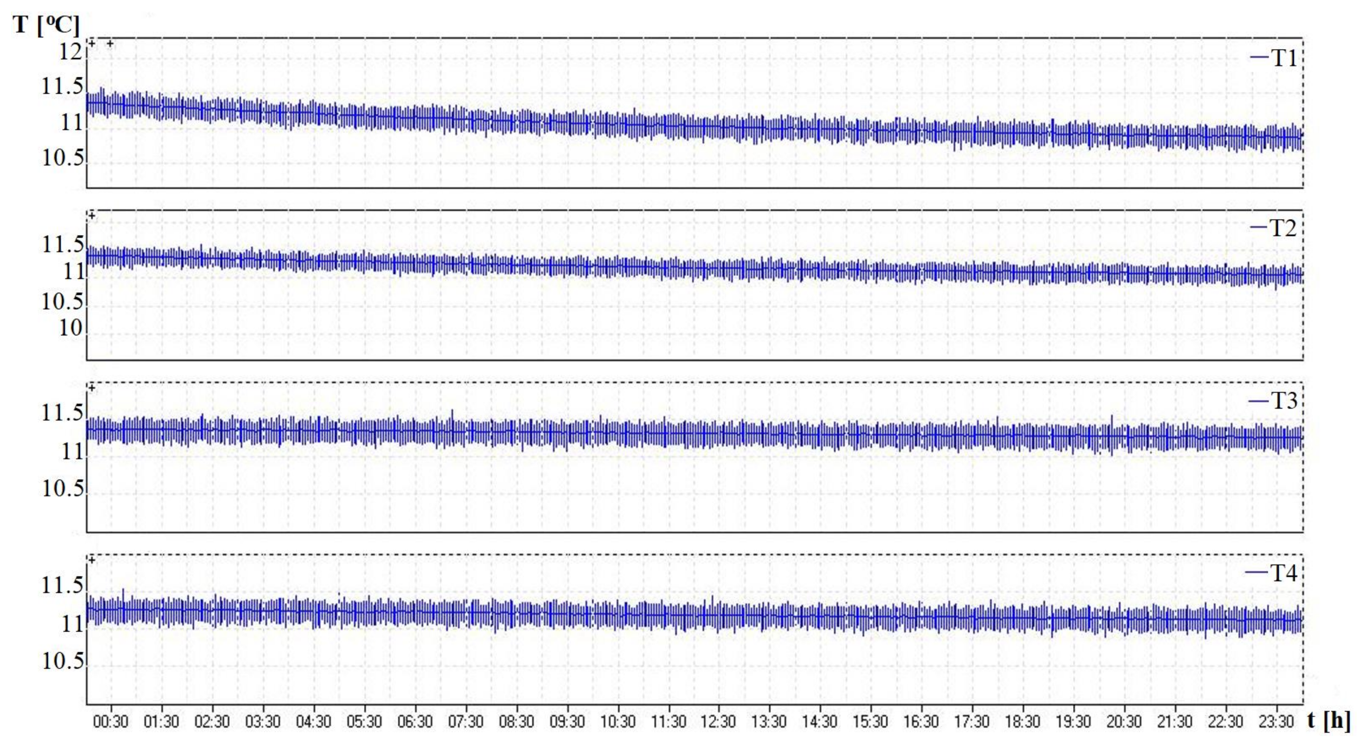
Experimental research followed under field conditions. The heating device was installed into the clay at a depth of 1 m, orienting the heated surface downwards (
Figure 3). The experiment was performed on 30 and 31 October. The temperature of the heated surface was kept at
T = 40 ± 1.5 °C. Experimental results are shown in
Figure 12.
The first charge continued
t = 301 s, the second:
t = 119 s, and the duration of the next was about sixty seconds. A total of
n = 33 charges were performed in four hours during the experiment. The total amount of charged heat was 0.25 kWh. As in the case of the laboratory experiment, the time interval between the charges increased and reached the almost constant value of 420 ± 10 s. The average heat flux density of the first hour was:
qav,h = 385 W/m
2, of the second:
qav,h = 231 W/m
2, of the third:
qav,h = 205 W/m
2, and of the fourth hour:
qav,h = 180 W/m
2 (
Table 3).
Through, analysing the heat dissipation in the ground (
Figure 13), it was observed that the heat reached the thermometer at a depth of 0.25 m from the centre of the heating surface after a time interval equal to
t = 1 h 48 min, and the thermometer at a depth of 0.50 m after:
t = 8 h 3 min. The thermometer at a depth of 0.25 m from the heating surface and on the side (
Figure 3) was reacted by heat after
t = 3 h for 34 min.
The temperatures were measured after the disconnection of the heating device, analysing the possibility of the soil keeping the heat (
Figure 12 and
Figure 13). During the first 20 h from the moment of disconnection of the heating device, the temperature of the soil layer next to the heated surface decreased from
Tc,0 = 41.1 °C to
Tc,0 = 11.5 °C due to heat dissipation into the surrounding soil layers: Δ
Tc,0= −29.6 °C. Heat dissipation also influenced change in temperature in the depth of 0.25 m from the centre of heated surface (
hc,0.25= −1.25 m). The temperature increased from
Tc,0.25 = 11.1 °C to
Tc,0.25,max = 12.1 °C and later decreased to
Tc,0.25 = 11.4 °C. At the same depth, but on the side (
hs,0.25= −1.25 m), the temperature changed similarly: from
Ts,0.25 = 11.1 °C to
Ts,0.25,max = 11.6 °C, then decreased to
Ts,0.25 = 11.3 °C. At 0.25 m deeper (
hc,0.50= −1.50 m), the temperature increased: from
Tc,0.50 = 11.1 °C to
Tc,0.50 = 11.3 °C: Δ
Tc,0.50= +0.2 °C. A decrease in temperature was observed during the next day (
Figure 13): Δ
Tc,0= −0.6 °C, Δ
Tc,0.25= −0.3 °C, Δ
Ts,0.25= −0.1 °C and Δ
Tc,0.50= −0.2 °C.
It could be concluded that heat dissipation in the soil is a slow process. The thermal charge of E = 0.25 kWh into the non-thermally separated soil volume dissipated within two days. Thermal energy could be stored longer by the thermal separation of a certain volume of the soil around the building.
3.3. Numerical Simulation
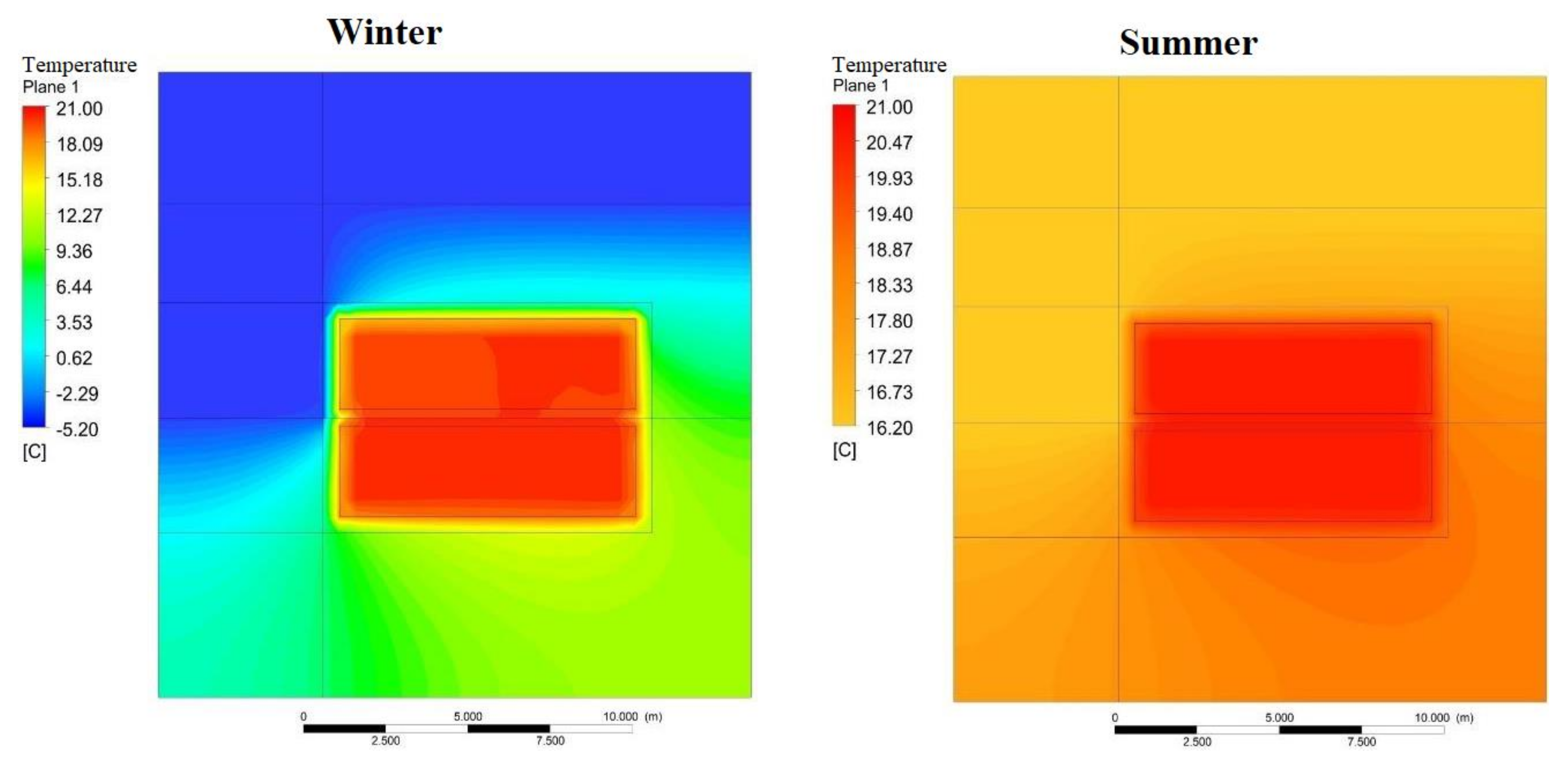
The simulation was performed from the initial conditions described in
Section 2.3 until thermodynamic balance. The results are shown in
Figure 14. In winter, in January, an airflow significantly cooled the soil surface. As a result, the temperature of the surface layers of the soil was relatively low due to the intensive heat transfer to the atmosphere. The upper part of the left façade of the building was also directly acted on by the cold wind. A higher increase in temperature was observed at the right side of the building and under the floor. Heat loss into the ground acted on the growth in soil temperature and accumulation of the heat there. As the soil temperature increased, the difference in temperatures of the air inside the building and the soil decreased. That meant that the heat loss into the soil generated conditions acting against the heat exchange. In the summer in July, an average air temperature was equal to
Tair = 16.2 °C. The building needed to be heated even during the summer to keep the air temperature inside the building at 21 °C. The temperature distribution was analogous to the case of the winter.
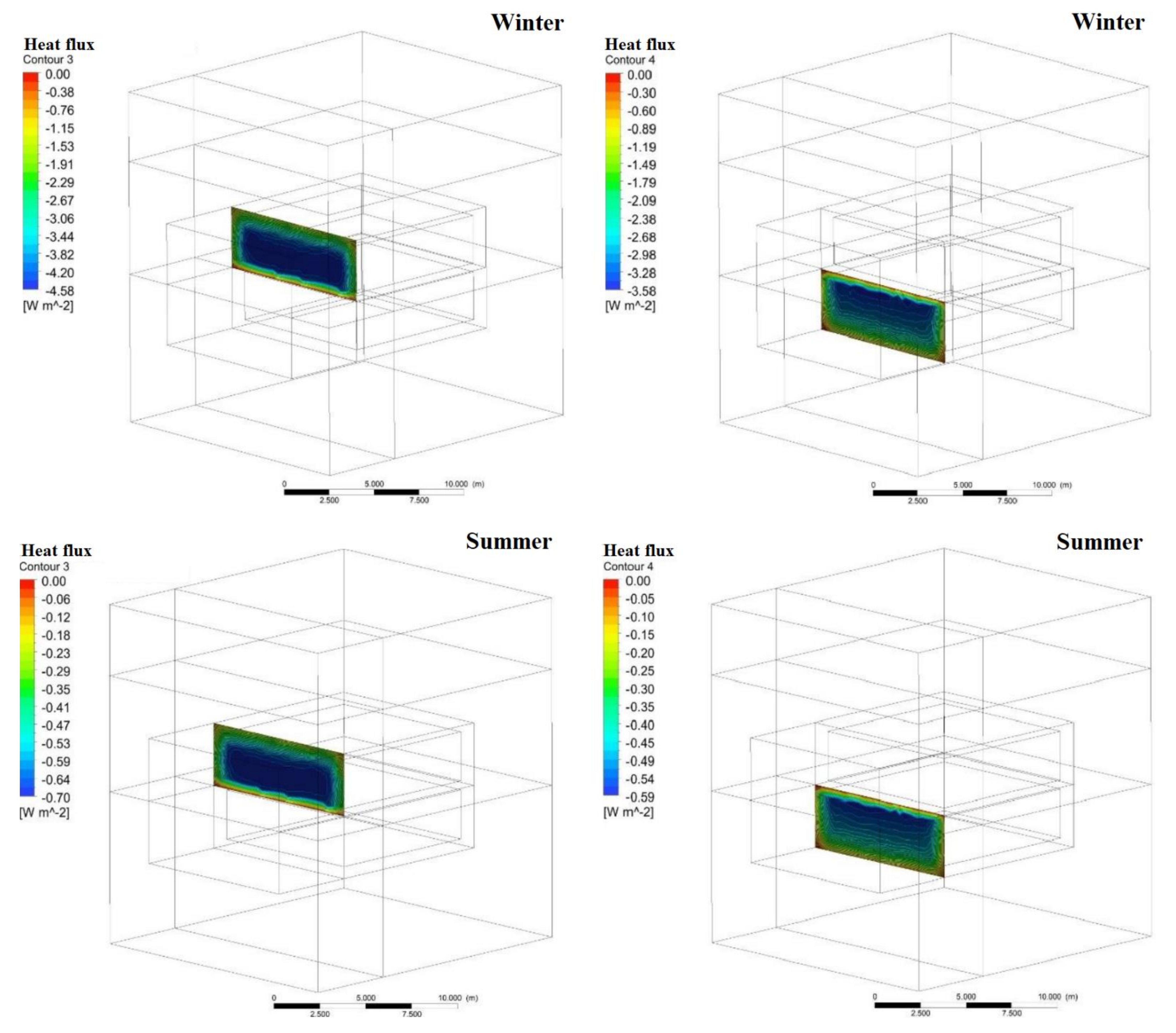
The heat flux density through each facade of the building into the soil was computed. The left façade was divided into two parts (
Figure 15) for the calculations. The airflow acted the part of the entrance into the building. An average value of the heat flux density through this part was equal to
qav= −4.58 W/m
2 in January. Here, the maximum heat loss to ambient was determined. The other part was underground. The heat flux density for this part was equal to
qav = −3.58 W/m
2. Heat loss through the roof of the building was high also:
qav = −3.61 W/m
2. The lowest heat flux density, with a maximum value only equal to
qmax = −1.75 W/m
2, was set through the floor in January.
In the model of the building, heating-consumed power was equal to P = 937 W for January. In the case of a typical building constructed on the ground, it was equal to P = 1304 W. An energy-saving level is 28 per cent in the case of underground buildings for January. Calculation of the energy demand for the air ventilation was not included in the computation. In both cases, the energy demand for air ventilation was assumed to be the same. Similar differences in energy demand were noticed for the spring and autumn seasons. The power of P = 153 W was required to maintain the same set temperature inside the building equal to 21 °C in July. In the case of the building constructed on the ground, it was equal to P = 245 W. The direct heat inflow into the typical buildings during the summer period was not evaluated in these computations, which may have a significant effect on the results. Therefore, the summertime results were not discussed further in the article.
The largest difference in temperature of the interior air of the building and the soil outside was found on the roof of the building. It determines the most intensive heat exchange and the highest heat loss there. It seems appropriate to insulate the roof thermally. The orientation of the building entrance to the contrary wind is also disadvantageous. It would also be beneficially to cover the ground surface with thermal insulation.
A certain volume of the soil around a building could be limited by thermal insulation material. The heat loss of the building would charge the soil by heat. Surplus energy from solar panels or photovoltaic cells could be used for the same purpose also. It would be possible to reduce the heat loss almost to zero by accumulating the heat and growing the soil temperature until it reaches the temperature of the building’s internal air.
4. Discussion
The soil layer charging by thermal energy and its storage was the objective of the research. The imaginary building was simulated numerically. The thermal properties of the building‘s partitions were described for the simulation. The building‘s shape of a parallelepiped was chosen to find the heat flux through each façade into the soil.
It should be mentioned that structural calculations and solutions are essential in the case of underground buildings and need to be performed. However, simulations of thermal processes in the case of the imaginary buildings are permitted to make some conclusions. The maximal heat flux density was through the roof. Therefore, it would be useful to cover it with a layer of thermal insulation and reduce the thickness of the soil layer here.
It was assumed that the soil type and thermal properties were constant, and the building was located above the groundwater level. Depth-dependent soil temperature was set for the numerical simulation.
The energy demand for the heating of the underground building was computed and compared with that of an analogous building constructed on the ground. In both cases, the energy demand for the building’s ventilation was assumed to be the same.
5. Conclusions
Soil’s temperature is higher than the air temperature in winter (heating season) and lower in summer (non-heating season). These conditions could be used to decrease the energy demand for heating or cooling of deepened or underground buildings. Therefore, analytical and experimental research was performed on thermal energy accumulation and the charge of the ground by heat.
During the experimental research in the laboratory, it was found that the most intensive heat charging followed from the beginning of the heating, due to the highest temperature difference between the heated surface and the soil. The average heat flux density of the charge of the cycle first hour was equal to 306 W/m2. As the nearest layer of the soil warmed up, the temperature difference decreased, affecting the decrease of charging intensity. Therefore, on the second hour of the cycle, the charge intensity was 3.5 times lower (equal to 88 W/m2) than in the first hour. It was noticed that a constant value of the average heat flux density reached a thermally stable state after six days. That meant the magnitude of the heat loss to the atmospheric air.
The underground building’s energy demand for space heating was computed. Building’s model was designed with one semi-exposed facade and a shape of a rectangular parallelepiped, with a length and width equal to nine and a height equal to six metres. The heating power needed for such a building was equal to 937 W in January. It was significantly lesser than that for an analogous building modelled on the ground. Calculation of the energy demand for the air ventilation was not included in the computations. In both cases, the energy demand for air ventilation was assumed to be the same. It was found that underground buildings could reach an energy saving of 28 percent.
Heat loss through the partitions of underground buildings heats the soil around. Heat spreads to colder layers dissipating over a larger soil volume. Higher ground temperature also worsens the conditions for heat transfer through the building partitions into the ground. The slow heat dissipation is the advantage in this case. Our research has shown that the small thermal charge in the non-thermally separated soil volume dissipated within two days. It seems that it would be valuable to limit the volume of the soil around the building with a layer of thermal insulation. This would prolong the heat accumulation time and reduce the heat loss through the building partitions into the ground, and would allow saving a part of the building’s energy for heating. In the case of the energy produced by burning fossil fuels, the decrease in energy used means a reduction of CO2 emissions.


 ,
, 


