Article

Spatial-Temporal Heterogeneity for Commercial Building Carbon Emissions in China: Based the Dagum Gini Coefficient

Department of Construction Management, School of Economics and Management, Beijing Jiaotong University, Beijing 100044, China
*
Author to whom correspondence should be addressed.
Sustainability 2022, 14(9), 5243; https://doi.org/10.3390/su14095243
Submission received: 13 February 2022 / Revised: 23 March 2022 / Accepted: 24 April 2022 / Published: 26 April 2022

Abstract

:
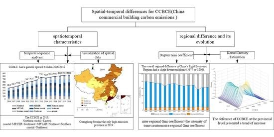
There is great potential for carbon emission reduction in commercial buildings. Determining the spatial-temporal heterogeneity of CCBCE (China’s commercial building carbon emissions) is crucial for developing differentiated emissions mitigation policies. This paper estimated CCBCE and then adopted a method involving the visualization of spatial data, Dagum Gini coefficient, and kernel density estimation to analyze the spatial-temporal characteristics and regional differences in China’s eight economic regions in 2006–2019. The results indicate that: (1) The CCBCE displayed a general upward trend, increasing from 400.99 million t (tons) to 853.23 million t. The CCBCE from electricity accounted for the largest share (65.93% in 2009). Moreover, Guangdong was the only high-emission province in 2019 with 77.8 million t CCBCE. (2) The contribution rate of the different economic regions to incremental carbon emissions made a significant difference, and inter-regional differences (61.81%) were much higher than intra-regional differences (7.99%). (3) The greatest intra-regional differences were found in the Southern coastal economic region (average Gini coefficient up to 0.4782). For inter-regional differences, the disparity between the Northern coastal economic region and Northwest economic region was greatest. Further, the regional differences presented a trend of increase. The study concludes that effective measures should be taken to reduce the CCBCE in each region and narrow the regional gap of CCBCE.

Graphical Abstract

1. Introduction

CO2, as an important cause of global warming, not only brings about air pollution, but also indirectly poses a threat to human health [1]. Countries around the world have formed a consensus on carbon emission reduction [2,3] and made efforts to achieve low-carbon targets [4]. According to the data published by CAIT (Climate Analysis Indicators Tool), China became the largest carbon emitter in 2006 [5]. In 2018, the carbon emissions increased to 9.66 billion t, approximately twice that of the United States. It is obvious that China is facing greater pressure to reduce carbon emissions [6], even if China has initiated some policies of carbon emission reduction and proposed the “double-control” strategy. Meanwhile, significant regional differences exist with regard to carbon emissions because different regions have different resource endowments, economic structures, and technical efficiency [3,7]. Judging from this, the unified emission reduction strategies would be too general to ease the pressure of carbon emissions in China [4]. Hence, if we formulate the emission reduction measures based on the carbon emission at the provincial level, it is not conducive to collaboration among provinces and macro-control at the national level, so the cost of measure-making will also increase [8]. Therefore, it is a suitable solution to discuss the spatial-temporal characteristics of carbon emission and propose carbon emission reduction strategies from the regional perspective.
However, the building sector, especially considering commercial buildings, is the major contributor to China’s carbon emissions [9]. As an important place for people working and entertainment, the energy consumption of commercial buildings is more than other types of buildings [10]. The commercial buildings were responsible for nearly 37.12% of total carbon emissions during the building operating phase in 2018 [11]. The energy consumption in large commercial buildings will reach as much as 4–6 times that of residential buildings. Meanwhile, the carbon emissions of commercial buildings in China will continue to grow in the future [12,13]. Moreover, compared with the residential buildings, commercial buildings have a larger potential for emissions reduction [14], but they have attracted less attention [9]. The relevant research has focused on driver factors [12,14] and decoupling analysis of CCBCE [15,16], and the research always focuses at the national level. The relevant research results make it difficult to guide carbon emission reduction in various regions. In the meanwhile, the CCBCE has been accompanied by a significant spatial clustering according to the space effect theory. Therefore, this paper attempts to study the spatial distribution and regional differences of CCBCE, which can provide the basis for various regions to formulate carbon emission reduction strategies in commercial buildings. However, the time-series data of CCBCE calculated by each institution is different, and regional division methods are controversial. Therefore, it is necessary to obtain more accurate calculation results of CCBCE and select the appropriate regions as research units. Moreover, what are the levels of CCBCE and their change trend? What are the levels, sources, and evolution patterns of regional differences in CCBCE? These issues should be addressed in the process of research. To respond to the above issues, this paper calculated the CCBCE of each province by modifying the previous research methods and took China’s eight economic regions as research objects. Then, we analyzed the level of CCBCE and its change using the methods of time series analysis and spatial data visualization. Afterward, the Dagum Gini coefficient was adopted to calculate the regional differences and their sources, and kernel density estimation was used to analyze the dynamic evolution of the differences. Both Dagum Gini coefficient and kernel density are calculated using Matlab 2016b.
Our study contributes to the previous papers in three ways. First, we improve the existing calculation methods of CCBCE, and the improvements are that we calculate the CCBCE from town (Town = urban + county + designated down [17]) heating consumption (the previous papers only calculated CCBCE from urban heating consumption), which is consistent with other energies in the geographical scope. Moreover, we consider the heat loss from the supply to end-use, and we deduct the natural gas and liquefied petroleum gas used in transportation, which have been included in building energy consumption in previous research. Second, we analyze the CCBCE and its change at national level and regional level and explore the CCBCE structure and the proportion of green power, which is conducive to reduce CCBCE at the source. Third, we employ the Dagum Gini coefficient to calculate the regional differences of CCBCE in eight comprehensive economic regions, which considers the overlap between samples to make up for the shortcomings of the Theil index and Gini coefficient, and we also analyze the dynamic evolution of regional differences by kernel density estimation, which reveals visually the long-term evolution trend of regional differences more specifically.
The research provides a new method to calculate CCBCE, namely calculation of the carbon emissions generated by various energies consumed by commercial buildings separately, and then adding them up to obtain CCBCE. Further, we use the more appropriate method to assess the regional differences of CCBCE and analyze their long-term evolution trend using kernel density estimation, which can more accurately reveal the regional characteristic of CCBCE to improve the effectiveness of policy making for regionally differentiated emissions reductions. In addition, as far as we know, these approaches have rarely been used in CCBCE analyses. In a practical sense, this study can not only help to achieve the goals of “peak carbon dioxide emissions” and being “carbon neutral” as soon as possible, but also provide references for other developing countries in the world. The remaining sections are organized as follows: Section 2 presents a literature review. We analyze and compare the existing calculation methods of CCBCE and summarize current concerns regarding regional difference analysis. Section 3 introduces the research methods, including improved calculation method for CCBCE, Dagum Gini coefficient, and kernel density estimation. Section 4 describes the results on the spatial-temporal pattern, regional disparities, and dynamic evolution of CCBCE from 2006 to 2019. Section 5 will conclude and put forward policy implications.

2. Literature Review

2.1. Calculation Methods of CCBCE

In China’s statistical system, the end-use energy consumption of the building is not calculated separately. Hence, the authoritative time-series data on building carbon emissions, especially on commercial buildings, are still lacking. To clearly master the CCBCE, plenty of scholars and institutions have made efforts to calculate the CCBCE.
The IEA (International Energy Agency) calculated the carbon emissions of 30 member states and eight alliance countries including China according to the end-use energy consumption, whose results were updated to 2019 [18]. TU-BERC (Tsinghua University-Building Energy Research Center) published the CCBCE (excluding heating) every year, and the latest data were from 2018 [19]. The Special Committee on Building Energy Consumption Statistics established by CABEE (China Association of Building Energy Efficiency) proposed a top-down method to calculate the CCBCE (including heating) from 2005–2019 based on the energy balance sheets [20]. However, the studies of the three institutions have their own advantages and disadvantages. The data of IEA have the highest timeliness, but do not reflect the actual status of CCBCE, because the energy balance sheets are different between the IEA and China [20]. TU-BERC employs the bottom-up method to calculate CCBCE (excluding heating). The data are more accurate compared with other studies, whereas the results are too small because they do not cover the carbon emissions from heating. The method of CABEE can obtain the time-series data easily, and it has authoritative data sources [21]. The results include the carbon emissions from heating. Therefore, the relevant research of CABEE has been recognized by numerous scholars. The recognition is mainly manifested in two aspects. First, the scholars use the calculation method of CABEE to calculate the CCBCE. For example, He et al. [10] used the method of CABEE to measure the carbon emissions of urban residential buildings, commercial buildings, and rural residential buildings. Both Wu et al. [22] and Tan et al. [23] referred to the method of CABEE to calculate the total carbon emissions during the operation phase of the building. Second, some scholars analyzed the CCBCE based on the first-hand data of CABEE. Ma and Cai [14] analyzed the driving force of carbon mitigation based on the national CCBCE in 2001–2015 issued by CABEE. Chen et al. [24] used the carbon emission and gross floor space data of residential and commercial buildings published by CABEE to predict the peak of CCBCE. Ma et al. [15] researched whether carbon intensity in the commercial building sector decouples from economic development in the service industry using the results from CABEE. Nevertheless, the data from CABEE have some disadvantages. Firstly, the reports only have the data of CCBCE at the provincial level from 2016 to 2018, which cannot be used to analyze the spatial distribution of CCBCE because of the small timespan. Secondly, it employs the urban centralized heating to modify the heating from China Energy Statistics Yearbook, whose data are lower, and it is inconsistent with the geographical scope of other energy statistics. Thirdly, the fuel and gas used in private transportation should be deducted, because the number of gas vehicles has risen sharply in recent years. The data concerning NGVs (natural gas vehicles) showed that the number of natural gas vehicles has reached 26.13 million around the world. Among them, China has 6.08 million natural gas vehicles, accounting for 23.2% [25]. Therefore, this study improves the calculation method to make up for the disadvantages of CABEE and then obtain the more concise CCBCE.

2.2. Exploration of Regional Differences

In recent years, the regional differences in carbon emissions have attracted the attention of a lot of scholars. Li et al. [4] and Huo et al. [26] found that the level of carbon emissions was different in each region, and the growth rate of regional carbon emissions had slowed down. Han et al. [27], Liu et al. [8], and Zhang et al. [7] analyzed the regional differences of carbon emissions in China and estimated the contribution of inter-regional differences and intra-regional differences using the Theil index. Their research focused on total carbon emissions from all industries. With the increase of carbon peak targets for key industries, the study scales of regional differences in carbon emissions have expanded to specific industries. For example, He et al. [28] explored the evolution mechanism and regional characteristics of carbon emissions in the power industry. Peng [29] studied the spatial-temporal heterogeneity, regional differences, and distribution dynamics of carbon emissions in the transportation industry. Li et al. [30] and Fan and Zhou [31] analyzed the spatiotemporal distribution and provincial contribution in the construction industry and building operation phase respectively. Moreover, there are fewer studies on regional differences in carbon emissions in commercial buildings, although it is the core sector of future carbon emission reductions.
In general, the existing studies have contributed to revealing the regional differences in China’s carbon emissions and provided policy implications to control the growth of carbon emissions. However, it is still controversial in the division of regions and research methods.
From the perspective of region division, previous literature mainly had three division patterns: three economic zones [26,32,33]; seven geographic regions [4,27]; and eight economic comprehensive zones [2,34,35,36]. The division pattern of three economic zones was proposed during the “7th FYP (Five Year Plan)”, which played a positive role to promote economic development in China. However, the results only reflect the rough outline of carbon emissions due to its rough division mode [8]. Then, for seven geographic regions, it avoids adopting a “one size fits all” emission reduction strategy for all regions, whereas the division is based on human, geographic, and political factors, which has a smaller impact on carbon emissions compared with economic growth. Finally, the division pattern of eight economic comprehensive zones was first proposed in Strategies and Policies for Regional Coordinated Development issued by the Development Research Center of the State Council during the 11th FYP period, and it was again highlighted in the 14th FYP. Therefore, it is in line with the current economic development of China and has more practical meaning to research the regional differences of CCBCE compared with the three economic zones and the seven geographic regions.
The research methods on region differences of carbon emissions have also been enriched in the past few years. The visualization of spatial data, Theil index, and Gini coefficient have been widely employed. Huo et al. [26] analyzed the spatial changes of carbon emissions of urban residential buildings and commercial buildings by visualizing the carbon emission value in end year of the FYP. Yang et al. [37] discussed the transfer status of hot spots in the northeast by visualizing the carbon emission data at the city level. The visualization of spatial data intuitively describes the regional differences in carbon emission and the changes in the carbon emission values of various provinces. Subsequently, calculating the regional difference level and analyzing its sources gradually became the focus of research. Zhang et al. [7], Wang et al. [38], Wang and Gong. [39], and Cui et al. [40] utilized the Theil index to calculate the regional differences and explored the contribution of inter-regional difference and intra-regional difference. Nevertheless, the Theil index does not take the intensity of transvariation into account, ignoring the problem of crossover between samples. Currently, some scholars in other fields have used the Dagum Gini coefficient to solve the overlooked problem of sample overlap. For instance, Si and Wang [41], Han et al. [42], and Wang et al. [43] employed the Dagum Gini coefficient to calculate respectively the regional differences of the economy of urban agglomeration, agricultural eco-efficiency loss, and PM2.5, and analyze their sources. Therefore, this paper will adopt the Dagum Gini coefficient to explore the regional differences of CCBCE.

3. Methods

The methods employed in this paper are the calculation of CCBCE, Dagum Gini coefficient, and kernel density estimation. The calculation of CCBCE provides the more reliable underlying data for analysis of regional differences and its dynamic evolution. The Dagum Gini coefficient is mainly used to measure the level of regional differences and analyze their sources, the research results are more scientific compared with the Theil index and Gini coefficient. The kernel density estimation can intuitively describe the dynamic evolution trends of regional differences. We usually analyze the distribution shape, location, and ductility of regional differences according to the kernel density curve, because it is a non-parametric estimation method and has no specific expression.

3.1. Calculation of CCBCE

The CCBCE, reported in this paper, refers to China’s commercial building carbon emissions in the building operation phase. We calculated the CCBCE from 30 provinces (m = 1, 2, …, 30) in 2006–2019. Owing to missing data, Xizang, Taiwan, Hong Kong, and Macao are not included in the study area. We set 2006–2019 as the study period (n = 2006, 2007, 2008, …, 2019) die to several causes. First, the Urban Construction Statistical System was revised by the MOHURD (Ministry of Housing and Urban-rural Development) in 2006, and the statistical indicators and statistical caliber have changed in this year. Second, the relevant data on the county and the designated town did not include in the China Urban-rural Construction Statistical Yearbook before 2006. Third, the newest China Energy Statistics Yearbook was published in 2020, but the data were only updated to 2019.
CCBCE mainly derives from various energies consumed during the building operation phase, such as raw coal, natural gas, electricity, LPG (liquefied petroleum gas), etc. We calculate the carbon emissions from each energy separately, then sum them up to get CCBCE. The calculation procedure and relevant symbols of CCBCE are shown in Figure 1.
In Figure 1, the parameters that need special explanation are as follows:
The E h e a t i n g , n , m c i t y , E h e a t i n g , n , m c o u n t r y , E h e a t i n g , n , m d e s i g n a t e d t o w n and r n , m c i t y , r n , m c o u n t y , r n , m d e s i g n a t e d t o w n are from the central heating sheet in China Urban-rural Construction Statistical Yearbook, and the “pe” is 92%, which comes from the Energy-saving design standards for residence in severe cold and cold regions (JGJ 26-2010). E F h e a t i n g , n equals the sum of carbon emissions from various energies for heating ( C h e a t i n g e ) to the heat supply ( H e ) (Equation (1)).
E F h e a t i n g , n = C h e a t i n g e H e
The E e l e c t r i c i t y , n , m T , R , E e l e c t r i c i t y , n , m T , P , E e l e c t r i c i t y , n , m T , P T comes from the Electricity consumption of the whole society in China Electricity Statistical Yearbook. E F e l e c t r i c i t y , n is calculated by (Equations (2) and (3)). C c e , n refers to standard coal consumption for electricity; E F S C is carbon emission factor for standard coal, which is 2.66 g CO2/gce. The data come from provincial CO2 emissions peaking program preparation guidelines. P T represents the percentage of thermal power, and E L T , n , E L H , n , E L W , n ,   and   E L N , n are power generation from thermal, hydro, wind, and nuclear respectively.
E F e l e c t r i c i t y , n = C c e , n × p T × E F S C 100
p T = E L T , n E L T , n + E L H , n + E L W , n + E L N , n

3.2. Dagum Gini Coefficient and Its Decomposition

Dagum proposed a new method (Dagum Gini coefficient) to further decompose the Gini coefficient of income inequality to compensate for the shortcomings of the traditional Gini coefficient and the Theil index [42]. Dagum Gini coefficient solves the cross-overlap problem among the samples when it is used to calculate the regional differences, and it also considers the specific distribution of subsamples fully. In this paper, we employ the Dagum Gini coefficient to analyze the regional differences of the CCBCE. The overall Dagum Gini coefficient ( G n ) can be expressed as follows:
G n = j = 1 k i = 1 m j h = 1 k r = 1 m h C C B C E n , j i C C B C E n , h r 2 m 2 C C B C E n ¯
where k is the serial number of regions. C C B C E n , j i C C B C E n , h r represents CCBCE for province i (r) of region j (h) in year n; C C B C E n ¯ represents the average value of CCBCE in year n; m j m h is the number of provinces in region i (r).
The overall Dagum Gini coefficient ( G n ) covers the contributions of the intra-regional differences ( G n , w ), inter-regional differences ( G n , n b ), and intensity of transvariation ( G n , t ). The equation is as follows.
G n = G n , w + G n , n b + G n , t
The G n , w , G n , n b , and G n , t can be calculated by Equations (6)–(8).
G n , w = j = 1 k G n , j j p j s j
G n , n b = j = 2 k h = 1 j 1 G n , j h p j s h + p h s j D n , j h
G n , t = j = 2 k h = 1 j 1 G n , j h p j s h + p h s j 1 D n , j h
Here, intra-regional Gini coefficient ( G n , j j ) and inter-regional Gini coefficient ( G n , j h ) were calculated by Equations (9) and (10). They respectively represent the intra-regional differences and inter-regional differences of CCBCE.
G n , j j = i = 1 m j r = 1 m j C C B C E n , j i C C B C E n , j r 2 m j 2 C C B C E n , j ¯
G n , j h = i = 1 m j r = 1 m h C C B C E n , j i C C B C E n , h r m j m h C C B C E n , j ¯ C C B C E n , h ¯
In Equations (6)–(8), p j = m j / m , s j = m j C C B C E n , j ¯ / m C C B C E n ¯ . Furthermore, D n , j h = d n , j h p n , j h / d n , j h + p n , j h , d n , j h represents the difference of CCBCE between the jth region and the hth region in year n, which is expressed as d n , j h = 0 d F j C C B C E n 0 C C B C E n C C B C E n x d F h x ) , where p n , j h indicates the first moment of transvariation, and it is calculated by p n , j h = 0 d F h C C B C E n 0 C C B C E n C C B C E n x d F j x ) .

3.3. Kernel Density Estimation

Kernel density estimation is a nonparametric estimating method used to measure the probabilistic density of random variables and we can utilize the kernel density curve to analyze the spatial nonequilibrium characteristics. We use kernel density estimation to measure the evolution patterns of differences in CCBCE.
First, suppose X is a random variable; x 1 , x 2 , x 3 , , x n is continuous sample observation values; the density function for X is f x = f x 1 , x 2 , x 3 , , x n ; the kernel density for f x at point x can be defined as:
f h ( x ) = 1 n h i = 1 n K x x i h
where K · refers to the kernel density, and h refers to bandwidth. To improve the accuracy of kernel density estimation, we employ the Gaussian kernel function as K · , which is calculated by Equation (12).
K x = 1 2 π exp x 2 2
The bandwidth has a significant impact on the accuracy of the kernel density function estimation, and the lower the bandwidth, the more accurate the estimation [44]. Therefore, if n , h = h n .

4. Results and Discussion

4.1. Spatial-Temporal Pattern Changes

4.1.1. Temporal Characteristic of Total CCBCE

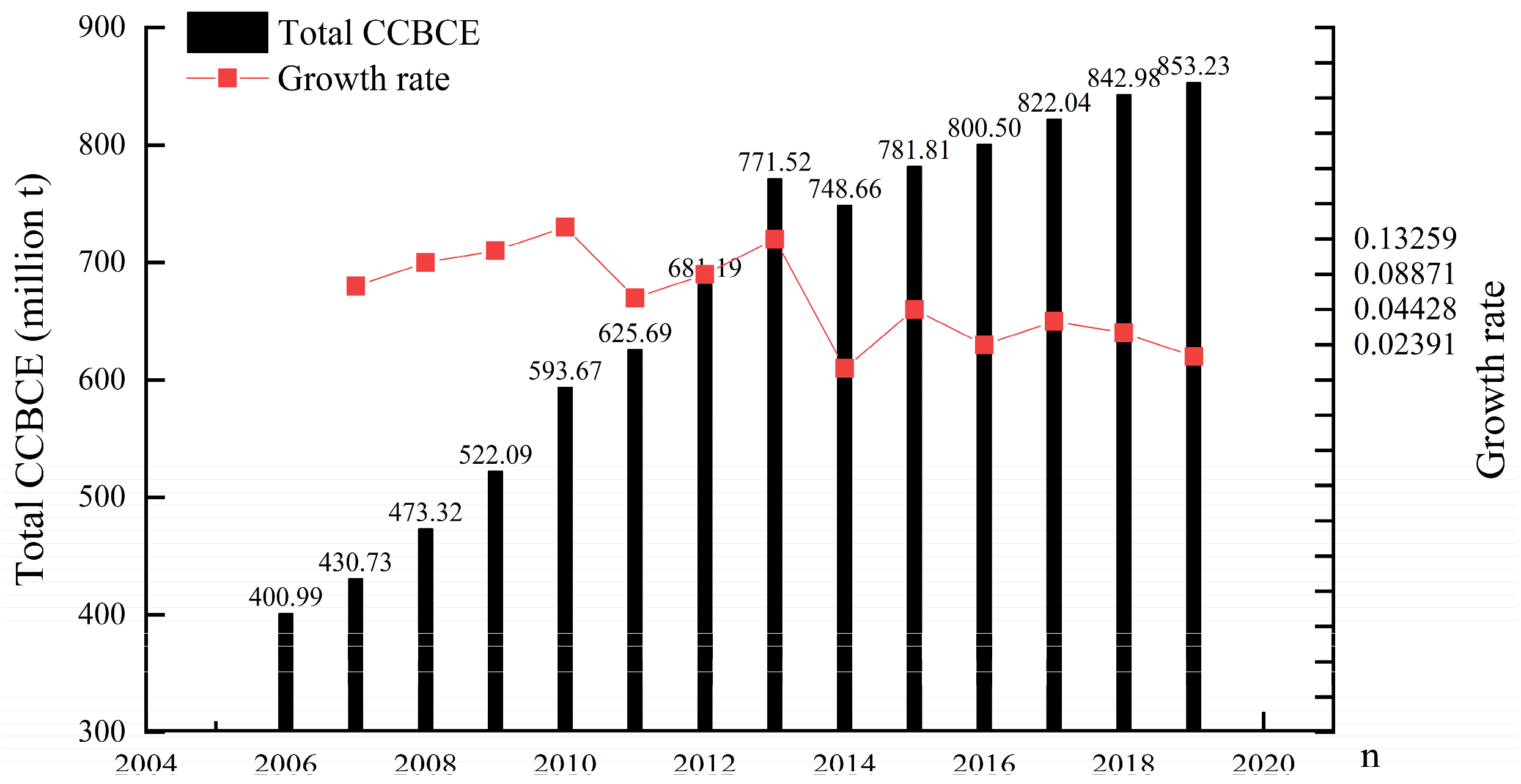
Figure 2 shows the total CCBCE levels and growth rates in 2006–2019. Overall, the total CCBCE had an upward trend during the study period, rising from 400.99 million t in 2006 to 853.23 million t in 2019, and the total CCBCE of 2019 was more than double that of 2006. However, the growth rate of total CCBCE had gradually declined, from 7.42% to 1.22%, which indicates that the total CCBCE will have a chance to peak in 2030. The total CCBCE showed a slight drop in 2014, to 748.66 million t from 771.52 million t in 2013. This may be attributed to several causes. First, China and the U.S. signed China-U.S. Joint Statement on Climate Change in 2014 [6]. Second, Energy Conservation Priority was established as the primary energy strategy by the National Energy Commission in 2014, and the Coal Power Energy Saving and Emission Reduction Upgrade and Renovation Action Plan started implement across the China [28]. Third, in 2014, the promulgation of Renovation of Old Pipe Networks for Urban Central Heating in Northern Heating Areas [45] and National New Urbanization Plan (2014–2020) [46] also promoted energy conservation and low-carbon development. China has successively formulated many strategic documents since the 18th National Congress of the Communist Party of China (2012), such as the National Climate Change Plan (2014–2020) and Enhanced Actions on Climate Change: China’s Intended Nationally Determined Contributions. China’s carbon emission growth rate significantly reduced under the guidance of these documents. The annual growth rate of CCBCE dropped from 9.2% (the “11th FYP” period) to 2.2% (the “13th FYP” period).
Figure 3 shows the sources of total CCBCE from three aspects: the proportion of CCBCE from each type of energies, CCBCE from electricity (the main source of total CCBCE), and the proportion of electricity generated by each power generation method. In Figure 3a, it is obvious that the total CCBCE was mainly generated by electricity, heating, and coal, the proportion of whom continuously stayed around 90%. This in turn represents the commercial buildings have little demand for oil, natural gas, and liquefied petroleum gas during the operation phase. Moreover, the change in the proportion of coal was roughly opposite to that of heating, having a general increasing trend except for a slight decrease in 2012 and 2018. Compared with coal and heating, electricity accounted for a greater proportion. The CCBCE from electricity increased from 209.97 million t to 562.39 million t in 2006–2019 with only decline in 2014, which was consistent with the change in total CCBCE (Figure 3b). This interesting finding reflects that electricity, as the absolute main source of total CCBCE, determined the changes in total CCBCE. Therefore, it is the most effective measure to reduce CCBCE that commercial buildings reduce electricity consumption. However, the thermal power has always been the main way to generate electricity in China. Though the proportion of thermal power dropped significantly in 2006–2019, from 83.4% to 68.8%, it occupied a large share, far surpassing hydropower, wind power, and nuclear power. The total proportion of wind power and nuclear power was less than 10%. This phenomenon illustrates the development of clean power is unmatured in China. This may be ascribed to the technology factor, security factor, etc. For example, the development of nuclear power is slow due to its unique safety conditions. The number of new hydroelectric power stations has been significantly reduced due to resettlement, environmental protection, and others. Moreover, both wind power and hydropower have technical shortcomings.

4.1.2. Spatial Distribution of CCBCE

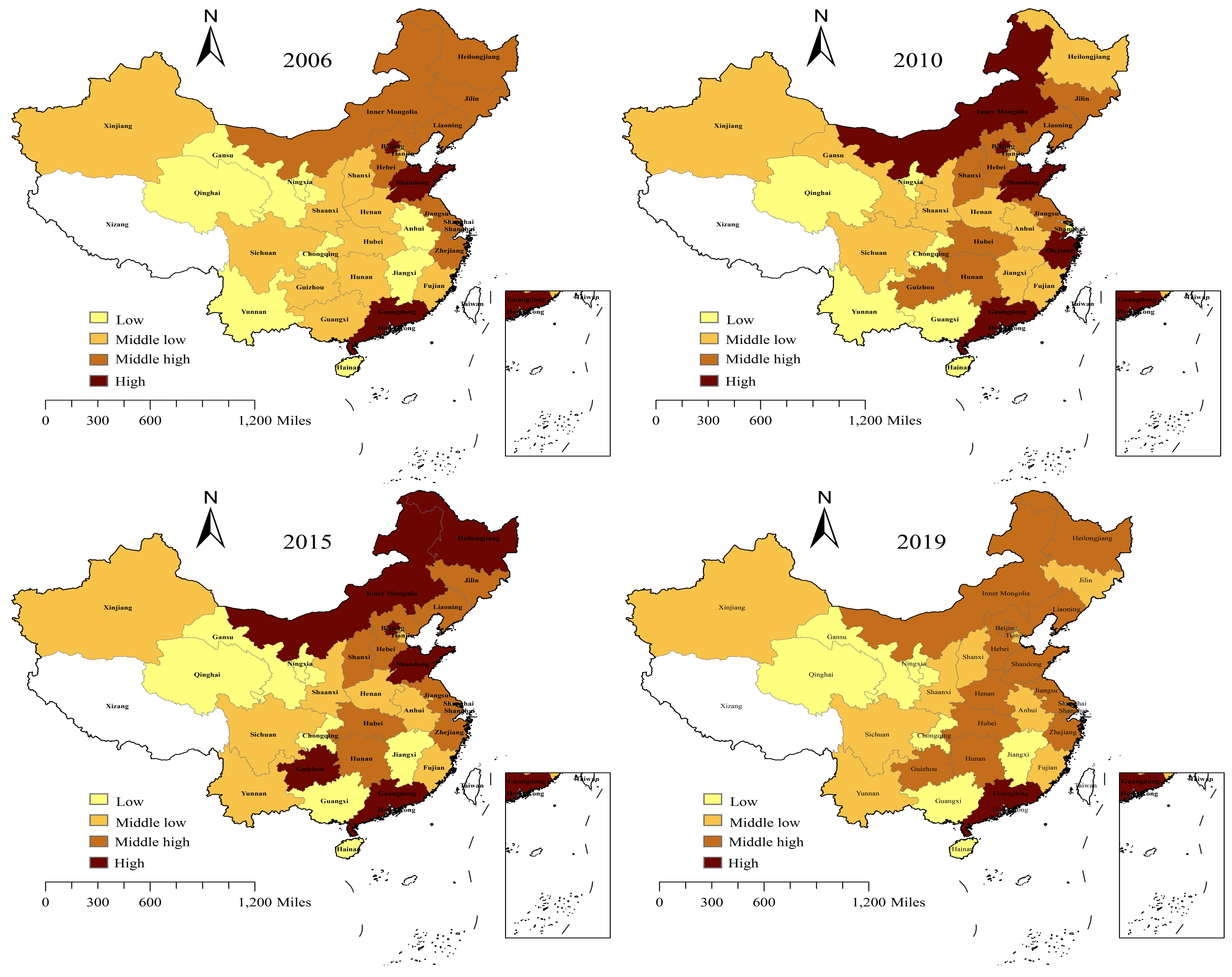
According to Section 3.1, we calculated the CCBCE in each province and drew respectively the geographic distribution map in 2006, 2010, 2015, and 2019 using ArcGIS 10.7 (See Figure 4). These provinces were divided into four levels using the method of natural fracture classification: “high emission provinces”, “middle high emission provinces”, “middle low emission provinces”, and “low emission provinces”. This method has been widely used by numerous scholars, such as Jiang et al. [47], Li et al. [48], and Peng [29]. The spatial distribution is shown in Figure 4.
As can be seen from Figure 4, the CCBCE in 2006–2015 showed a significant upward trend, the number of provinces with high CCBCE increased from 4 to 6. During the “13th FYP” period (2016–2019), the number had an obvious downward, decreasing from 6 (Inner Mongolia, Heilongjiang, Beijing, Shandong, Zhejiang, Guangdong) in 2015 to 1 (Guangdong) in 2019. Among six high-emission provinces in 2015, the CCBCE dropped 36.5% and 27.5% in Inner Mongolia and Heilongjiang, respectively, while Guangdong did not decline but increased, increasing from 65.35 million t in 2015 to 77.81 million t in 2019, and the annual growth rate was up to 4.7%. Inner Mongolia and Heilongjiang are located in the severe cold areas of China with high demand for heating. Their decrease in 2015–2019 may be caused by the requirement of Design Standards for Energy Efficiency of Public Buildings approved by MOHURD in 2015: commercial buildings would reduce the 75% heating consumption. Compared with the coastal areas, such as Guangdong, the CCBCE of Northwest areas (Gansu, Qinghai, et al.) were low, which may be ascribed to the relatively underdeveloped economy in the service sector.

4.2. Regional Heterogeneity of CCBCE

4.2.1. Division of Regions

To explore the regional differences of CCBCE, this paper selected China’s eight comprehensive economic zones as research subjects, which was defined by the Development Research Center of the State Council. The detailed information is as follows: Northeast economic region (Northeast); Economic region in the middle reaches of the yellow river (MRYER); Northern coastal economic region (Northern coastal); Economic region in the middle reaches of the Yangtze River (MRYAR); Eastern coastal economic region (Eastern coastal); Southwest economic region (Southwest); Southern coastal economic region (Southern coastal); Northwest economic region (Northwest). The specific provinces included in every economic region are shown in Table 1.

4.2.2. CCBCE in China’s Eight Comprehensive Economic Zones

Figure 5 shows the contribution of eight comprehensive economic zones to increments of total CCBCE. At the regional scale, the contribution of different economic zones to the increase of CCBCE was different, and the contribution changed over time. From 2006 to 2010, the total CCBCE increased 192.68 Mt, approximately 48.05%. The contribution of the Northern coastal region was 27.46%, the largest one of the eight economic zones. By comparison, the contribution of the Eastern coastal and the Northwest regions were lower than other regions, and the contribution rates were respectively 1.13% and 3.83%. The Northeast contributed the most CCBCE in 2010–2015, increasing to 31.93% from 6.29%. The contribution of Northern coastal dropped significantly, from 27.46% in 2006–2010 to 2.23% in 2010–2015. The Northwest contributed the smallest CCBCE in 2010–2015, which could be due to the lower urbanization rate caused by slower economic growth. In 2015–2019, the CCBCE increased to 71.43 million t, with the lowest increase rate in three periods. Moreover, the CCBCE of both Northeast and MRYER presented negative growth, and the contribution of Northern coastal also changed from the largest in 2006–2010 to the smallest in 2015–2019. This finding further illustrates that China has implemented carbon emission reduction strategies for areas with high carbon emissions in the past ten years. It is not difficult to see that the CCBCE of the eight comprehensive economic zones demonstrate obvious differences.

4.3. Decomposition of Regional Differences

4.3.1. Overall and Intra-Regional Differences in CCBCE

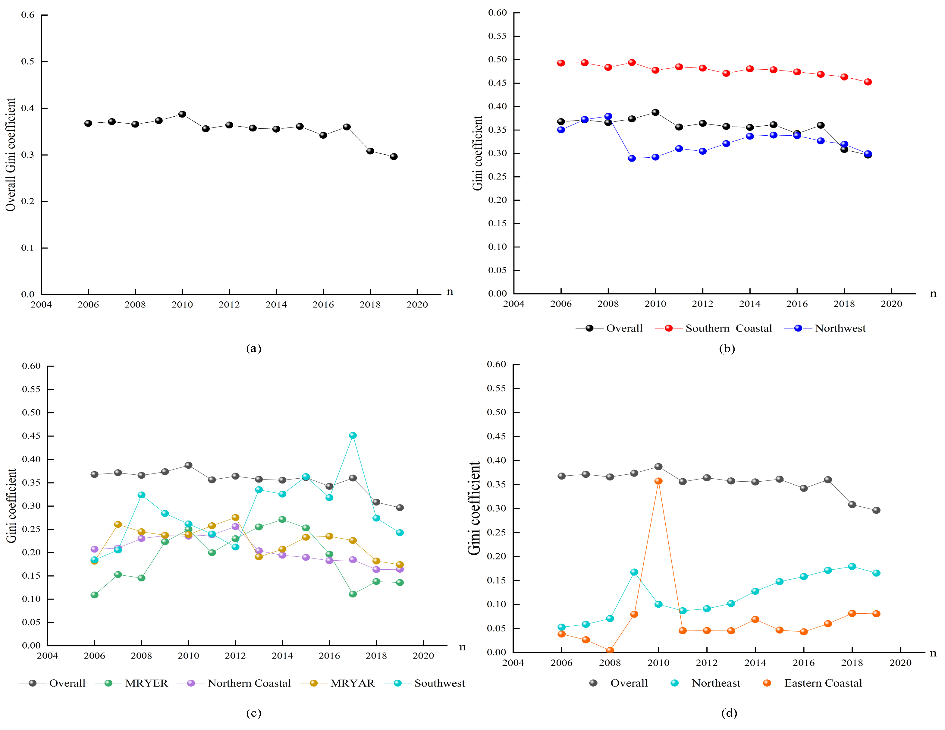
Figure 6 describes the trends of the overall and intra-regional Gini coefficient of the CCBCE in 2006–2019. The overall Gini coefficient of CCBCE shows a slight downtrend during the study period, dropping from 0.3677 in 2006 to 0.2964 in 2019. The overall Gini coefficient fluctuated between 0.34 and 0.37 in 2006–2017, and it significantly decreased with an average annual decline rate of 8.8% since 2018. This reflects that China’s carbon emissions differences in commercial buildings have been reduced obviously under the guidance of regional coordinated development strategy and new urbanization strategy put forward by the “19th National Congress of the Communist Party of China”. In terms of the intra-regional Gini coefficient, it could be seen that both Southern coastal and Northwest are at the high level, while Southwest, Northern coastal, MRYAR, and MRYER are in the middle zone, and Eastern coastal and Northeast are at the low level. The main findings are presented as follows:
In high-level regions, Southern coastal had the largest intra-regional difference. The difference declined slowly during the study period, and the Gini coefficient still maintained at 0.4525, surpassing the overall Gini coefficient. The Gini coefficient of the Northwest was roughly at the same level as the overall Gini coefficient, except for a drastic decline in 2009, and it showed a trend of fast fall followed by a slow rise.
In the middle zone, the Gini coefficient of MRYER and MRYAR was constantly fluctuating in 2006–2019, and the fluctuation ranges were respectively 0.1091–0.2711 and 0.1815–0.2756. The Gini coefficient of Northern coastal showed an upward trend in 2006–2012, rising from 0.2071 in 2006 to 0.2561 in 2012, following a downtrend in 2012–2019, dropping from 0.2561 in 2012 to 0.1642 in 2019. Overall, the Gini coefficient of Southwest showed a fluctuating increasing trend in 2006–2019, from 0.1844 in 2006 to 0.2428 in 2019. The fluctuations were extremely obvious during the study period, manifesting as sharp increases in 2007, 2012, and 2016.
In low-level regions, Eastern coastal had the smallest Gini coefficient, and it reached the lowest point in 2018. After that, it fluctuated, rising to 0.0809 in 2019. The Gini coefficient of Northeast showed a general increasing trend in 2006–2019, rising 0.0527 to 0.1656 with an average annual growth rate of 16.48%. Moreover, the Gini coefficient of Northeast was almost the same as that of Northern coastal.

4.3.2. Inter-Regional Differences in CCBCE

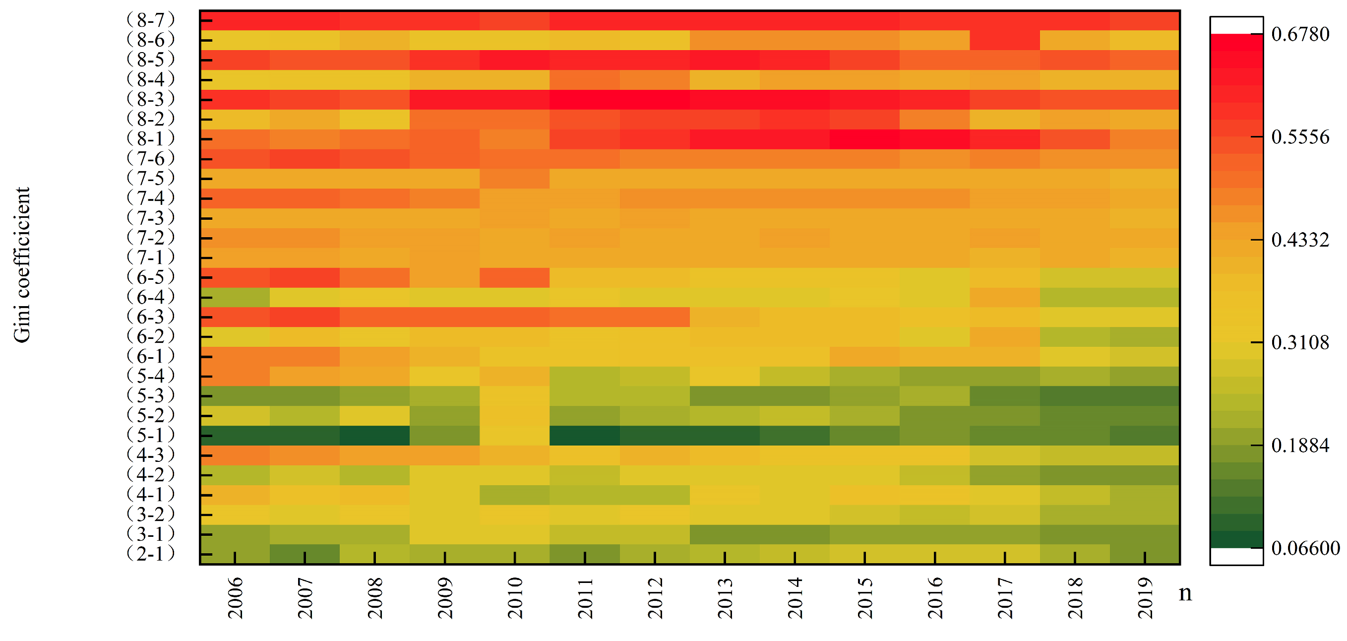
Figure 7 describes the trends of the inter-regional Gini coefficient of CCBCE in 2006–2019. It can be seen that the (8-7) ((Northwest)-(Southern coastal)), (8-5) ((Northwest)-(Eastern coastal)), and (8-3) ((Northwest)-(Northern coastal)) had a larger inter-regional Gini coefficient than others, and the Gini coefficient always stayed at a high level during the study periods. Their average annual Gini coefficients were separately 0.5927, 0.5720, and 0.6067. This finding reflects that the unbalanced status between Northwest and coastal region always existed and did not alleviate, which may be caused by the uneven economic development in service sectors between inland and coastal areas. It also illustrates that the regional development strategy has not fundamentally changed the uneven development status between east and west regions, though it has narrowed the gap among the neighboring cities, such as Shanghai and Zhejiang in Eastern coastal regions.
In contrast, the smallest Gini coefficient existed in (5-1) ((Eastern coastal)-(North-east)). The main reason for this might be that both Northeast and Eastern coastal have larger CCBCE, which can be explained that the Northeast belongs to a severely cold area with a large demand for heating, and the people in the Eastern coastal region have a greater demand for shopping and entertainment because of the relatively developed economies and high urbanization rates. In addition, its Gini coefficient experienced slight growth, especially in 2013–2017. It increased from 0.0886 in 2013 to 0.1621 in 2017. This indicates the CCBCE in Eastern coastal has reduced because of the scale economy effect, which leads to the increase of difference between Eastern coastal and Northeast.
In Figure 7, we also find that the Gini coefficient of (5-4) ((eastern coastal)-MRYAR) had the most obvious decline in 2006–2019, down from 0.4763 to 0.2713, with an average annual decline rate of 4.38%. Compared with (5-4) ((eastern coastal)-MRYAR), the other inter-regional Gini coefficient did not change significantly during the study periods.

4.3.3. Sources of the Differences in CCBCE and Their Contribution Rates

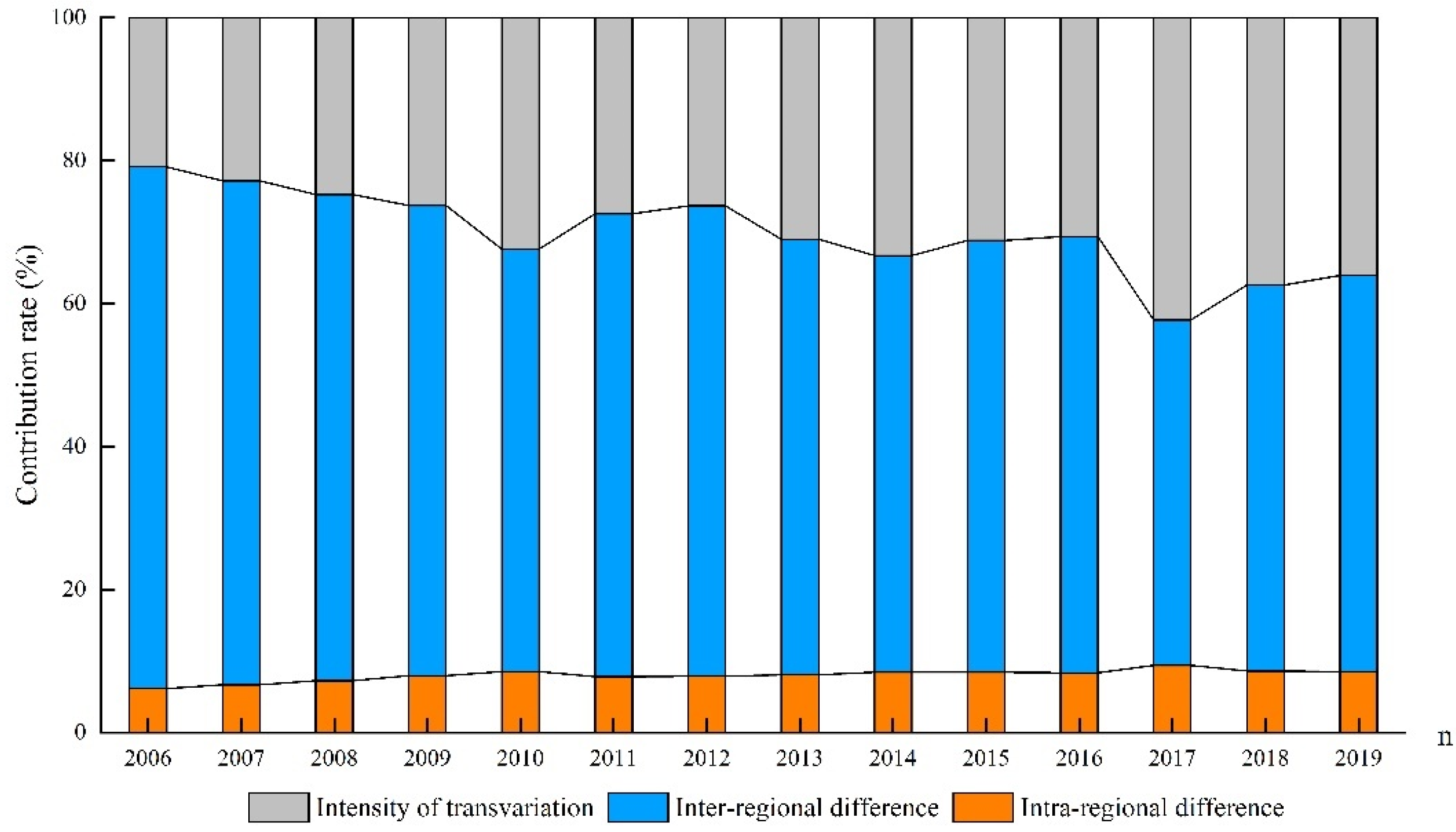
Figure 8 shows the sources of the differences in CCBCE and the trends of their contribution rates. During the study period, the mean contribution rates of the inter-regional differences, intensity of transvariation, and intra-regional differences towards regional differences in CCBCE were 61.81%, 30.19%, and 7.99%, respectively. Moreover, the mean contribution rate of inter-regional differences roughly was eight times that of intra-regional differences. From the evolution processes, it should be noted that the contribution of the intra-regional differences remained below 10% with an extraordinary slow growth trend. This in turn illustrates that if governments take respective carbon emission reduction measures for commercial buildings in eight comprehensive economic zones, the carbon emission reduction needs of the provinces in the region will be better met. However, the contribution rate of the inter-regional differences maintained a high level continuously and showed a dynamic evolution process of repeated increases and decreases. During 2006–2010, it gradually dropped from 72.97% to 59.10% with an average annual down rate of 4.75%, and it fluctuated between 58.29% and 65.81% in 2010–2016. From 2016 to 2019, it showed a slow growth after a significant fall, and it decreased to the lowest point (0.4834) in 2017. The intensity of transvariation towards regional differences presented an overall increasing trend, from 20.88% to 36.06%, which far exceeded intra-regional differences. Therefore, the sample overlap problem was relatively significant, which was not ignored in the analysis of regional heterogeneity. On the other hand, it also reflects that the results calculated by Dagum Gini coefficient were more in line with reality than those calculated by the Theil index and Gini coefficient.

4.4. Dynamic Evolution

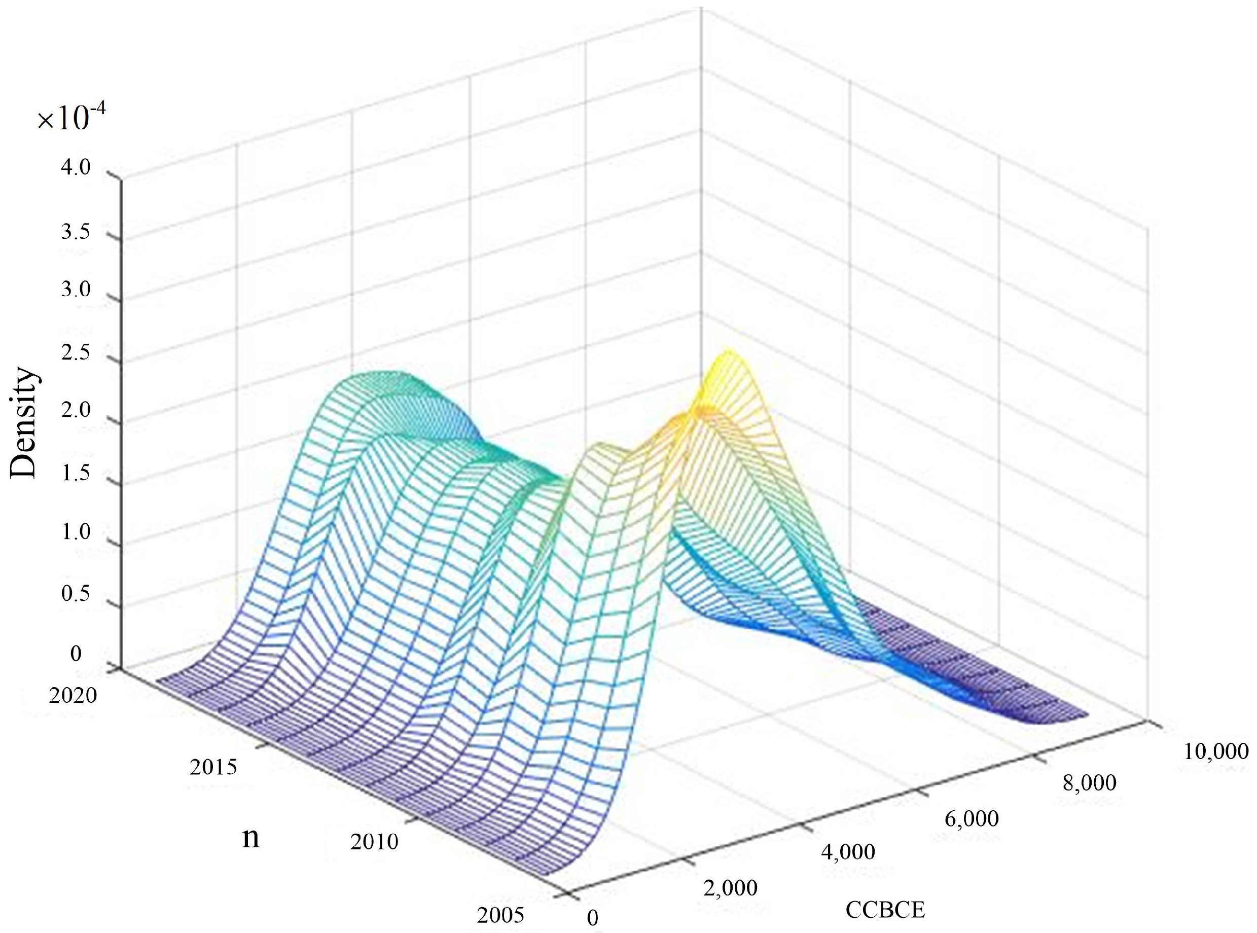
Figure 9 shows the evolution path of differences in 30 provinces in 2006–2019. During the study period, the peak of the kernel density curve gradually decreased, the central point of the density function moved towards the left, and the peak became wider and wider. These indicate that the differences of CCBCE presented a trend of increase. Specifically:
In 2006–2010, the kernel density curve showed a leftward shift, and the height of the peak dropped significantly over time. This reflects the differences of CCBCE increasing obviously during the 11th FYP period.
In 2011–2017, over time, the height of the peak fluctuated in a small range, and the movement of the central point of the density function was not obvious. This phenomenon illustrates that China has made vigorous efforts to narrow the gap of differences in CCBCE.
In 2018–2019, the peak value showed a generally upward trend, and the growth of the width of the peak was extraordinarily obvious, which further illustrated that the issue of differences of CCBCE cannot be ignored, although it has been slightly alleviated in the past few years.

5. Conclusions and Policy Implications

5.1. Conclusions

Previous studies have more attention to the analysis of total CCBCE and provided a series of proposals to alleviate the pressure on CCBCE from the national level. At present, the strategy of intra-regional coordinated emission reduction has been incorporated into the policy plan for “peak carbon dioxide emissions” and being “carbon neutral”, and the pressure to reduce carbon emissions has penetrated into all provinces and all fields. The study of regional differences in CCBCE is worthy of attention. In this paper, we select eight economic comprehensive regions as research objects by comparing the advantages and disadvantages of various regional division methods in the section literature review, which not only take space effects into account, but also avoid a single, one-size-fits-all solution. Moreover, the level and contribution rate of intra-regional and inter-regional differences of CCBCE can be obtained through the decomposition of regional carbon emission differences, which provides convenience for reducing regional differences. Moreover, total and provincial CCBCE calculated by the improved calculation method provided a more reliable data basis for the analysis of spatiotemporal patterns, regional differences, and their dynamic evolution.
The main research findings of this paper are of practical use for the control of carbon emissions from commercial buildings. (1) The CCBCE showed a general upward trend, up to 853.23 million t in 2019. The proportion of CCBCE from electricity to total CCBCE was on the rise, increasing from 52.36% in 2006 to 65.93% in 2019, approximately accounting for two thirds of the total CCBCE. Moreover, thermal power was still the most important form of power generation in China, with its average proportion being 77.3%. Thus, focusing on reducing electricity consumption in commercial buildings and developing clean electricity is required. (2) The number of provinces with high CCBCE decreased, but the CCBCE in severely cold areas and economically developed areas were still high. The main provincial contributors were Guangdong (77.81 Million t), Shandong (52.23 Million t), and Heilongjiang (48.43 Million t) in 2019. These should become the key areas for commercial building carbon emissions reduction in the future. (3) The intra-regional differences of CCBCE remain stable from 2011 to 2019, whose contribution rate always stayed below 10%. The inter-regional differences were much higher than intra-regional differences, and the largest inter-regional existed in the Northwest and coastal areas during the study period: Eastern coastal–Northwest, Northern coastal–Northwest, and Southern coastal–Northwest. Governments must play an important role for to implement carbon emission reduction measures of commercial buildings in eight comprehensive economic zones respectively. Moreover, narrowing the development gap between coastal and inland is also one of the means to achieve “peak carbon dioxide emissions” as soon as possible.

5.2. Policy Implications

Based on the above findings, policy recommendations for reducing the CCBCE and promoting CCBCE to peak are proposed in this paper:
The government should actively promote the electrification of commercial buildings and increase the proportion of green electricity usage. Coal and electricity represent the main energy consumed by commercial buildings, which generate a lot of carbon emissions during the commercial building operation phase. However, it is well-known that the carbon emission factor of electricity is lower than that of coal and it is declining year by year. In 2019, the carbon emission factor of electricity was only one quarter of that of raw coal. Therefore, government encouragement to replace coal with electricity in end-use consumption of commercial buildings will be an effective way to reduce CCBCE. Further, based on the seriously small proportion of clean energy power generation, China should increase the support for clean energy companies, especially leading companies, and encourage them to broaden financing channels by using industrial investment funds.
Countries should formulate targeted local carbon mitigation policies based on regional heterogeneity. Firstly, the government should have a comprehensive understanding for the basic patterns and key issues of CCBCE in each region and respectively take actions to reduce carbon emissions, rather than adopting a single, one-size-fits-all solution. At the same time, it is necessary to actively carry out cooperation in various regions and establish a regional environmental protection linkage mechanism. For coastal areas with developed economies, we should continue to enhance the development of high-tech and independent innovation, try to establish a hydrogen industrial system and a complete industrial chain, and actively develop ultra-low energy consumption, near-zero energy consumption buildings. At the same time, the local governments should make full use of foreign capital and strengthen the awareness of energy conservation and emission reduction of foreign-invested enterprises. For severe cold areas with high heating demand, we should retrofit the walls, roofs, and windows in commercial buildings to improve heating efficiency. In addition, the Northeast economic region should carry out waste heat recovery and explore geothermal and solar heating to substitute coal-fired heating.
Promoting energy saving in offices is also an important way to reduce CCBCE. Occupants in offices usually have weaker energy-saving awareness because they do not pay for the use of energy. Thus, the companies or institutions should carry out energy-saving training for occupants and implement energy-saving incentives for departments or individuals with good energy-saving performance. In addition, all units can set up an energy efficiency website to display and share office energy saving tips referring to the practice of the Hong Kong Electrical and Mechanical Services Department [9].
Various aspects of this study may be improved in future research. First, the calculation results of CCBCE are only updated to 2019 because the relevant statistics for 2020 and 2021 have not been released by the National Bureau of Statistics. The integration of multiple sources of data should be taken into account in future research to make up for the shortcomings of statistical data. The multiple sources of data cover the statistical data, survey data, and the data obtained by the Internet or Internet of Things. Second, this paper set eight comprehensive economic zones as research objects. In future research, we can select more scientific and dynamic area division methods with the help of mathematical methods and analysis software. In addition, the regional difference measurement method is still being optimized, so it is necessary to pay attention to overcome their limitations in application.

Author Contributions

This study was designed by T.M., Y.L. and M.Y. retrieval of data from yearbooks, M.Y.; methodology, T.M.; software, T.M. and M.Y.; writing—review and editing, Y.L.; writing—original draft, T.M. All authors have read and agreed to the published version of the manuscript.

Funding

This work was supported by the China National Key R&D Program under grant no.2018YFC0704300 and National Natural Science Foundation of China under grant no. 71871014.

Institutional Review Board Statement

Not applicable.

Informed Consent Statement

Not applicable.

Data Availability Statement

All the data adopted in this article are from public resources and have been cited with references accordingly.

Conflicts of Interest

The authors declare no conflict of interest. The funders had no role in the design of the study; in the collection, analyses, or interpretation of data; in the writing of the manuscript, or in the decision to publish the results.

References

  1. Zou, C.; Xue, H.; Xiong, B.; Zhang, G.; Pan, S.; Jia, C.; Wang, Y.; Ma, F.; Sun, Q.; Guan, C.; et al. Connotation, innovation and vision of “carbon neutrality”. Nat. Gas Ind. B 2021, 8, 523–537. [Google Scholar] [CrossRef]
  2. Zeng, L.; Lu, H.; Liu, Y.; Zhou, Y.; Hu, H. Analysis of Regional Differences and Influencing Factors on China’s Carbon Emission Efficiency in 2005–2015. Energies 2019, 12, 3081. [Google Scholar] [CrossRef] [Green Version]
  3. Han, X.; Yu, J.; Xia, Y.; Wang, J. Spatiotemporal characteristics of carbon emissions in energy-enriched areas and the evolution of regional types. Energy Rep. 2021, 7, 7224–7237. [Google Scholar] [CrossRef]
  4. Li, X.; Wang, J.; Zhang, M.; Ouyang, J.; Shi, W. Regional differences in carbon emission of China’s industries and its decomposition effects. J. Clean. Prod. 2020, 270, 122528. [Google Scholar] [CrossRef]
  5. CAIT. (Climate Analysis Indicators Tool). Available online: https://www.climatewatchdata.org/ghg-emissions?end_year=2018&start_year=1990 (accessed on 12 December 2021).
  6. Dong, F.; Hua, Y.; Yu, B. Peak Carbon Emissions in China: Status, Key Factors and Countermeasures—A Literature Review. Sustainability 2018, 10, 2895. [Google Scholar] [CrossRef] [Green Version]
  7. Zhang, Y.; Yu, Z.; Zhang, J. Analysis of carbon emission performance and regional differences in China’s eight economic regions: Based on the super-efficiency SBM model and the Theil index. PLoS ONE 2021, 16, e0250994. [Google Scholar] [CrossRef]
  8. Liu, X.; Yang, X.; Guo, R. Regional Differences in Fossil Energy-Related Carbon Emissions in China’s Eight Economic Regions: Based on the Theil Index and PLS-VIP Method. Sustainability 2020, 12, 2576. [Google Scholar] [CrossRef] [Green Version]
  9. Lu, M.; Lai, J. Review on carbon emissions of commercial buildings. Renew. Sustain. Energy Rev. 2020, 119, 109545. [Google Scholar] [CrossRef]
  10. He, J.; Yue, Q.; Li, Y.; Zhao, F.; Wang, H. Driving force analysis of carbon emissions in China’s building industry: 2000–2015. Sustain. Cities Soc. 2020, 60, 102268. [Google Scholar] [CrossRef]
  11. CABEE, Chinese Building Energy Consumption Report (2020). 2020. Available online: https://www.cabee.org/site/content/24085.html (accessed on 20 November 2021). (In Chinese).
  12. Ma, M.; Cai, W.; Cai, W. Carbon abatement in China’s commercial building sector: A bottom-up measurement model based on Kaya-LMDI methods. Energy 2018, 165, 350–368. [Google Scholar] [CrossRef]
  13. Li, X. Research on Carbon Emissions Trading Mechanism of Urban Public Buildings in China; Beijing Jiaotong University: Beijing, China, 2021. (In Chinese) [Google Scholar]
  14. Ma, M.; Cai, W.; Cai, W.; Dong, L. Whether carbon intensity in the commercial building sector decouples from economic development in the service industry? Empirical evidence from the top five urban agglomerations in China. J. Clean. Prod. 2019, 222, 193–205. [Google Scholar] [CrossRef]
  15. Ma, M.; Cai, W. What drives the carbon mitigation in Chinese commercial building sector? Evidence from decomposing an extended Kaya identity. Sci. Total Environ. 2018, 634, 884–899. [Google Scholar] [CrossRef] [PubMed]
  16. Ma, M.; Cai, W. Do commercial building sector-derived carbon emissions decouple from the economic growth in Tertiary Industry? A case study of four municipalities in China. Sci. Total Environ. 2019, 650, 822–834. [Google Scholar] [CrossRef] [PubMed]
  17. NBS (National Bureau of Statistics), The Division of Town and Rural Areas in The Statistical. Available online: http://www.stats.gov.cn/tjsj/tjbz/200610/t20061018_8666.html (accessed on 5 January 2022). (In Chinese)
  18. IEA (International Energy Agency). Available online: http://www.iea.org/publications/freepublications/publication/Building2013_free.pdf%5Cnwww.iea.org/etp/buildings (accessed on 10 January 2022).
  19. Tsinghua University-Building Energy Research Center. Annual Report on China Building Energy Efficiency; China Building Industry Press: Beijing, China, 2020. (In Chinese) [Google Scholar]
  20. Huo, T.; Ren, H.; Zhang, X.; Cai, W.; Feng, W.; Zhou, N.; Wang, X. China’s energy consumption in the building sector: A Statistical Yearbook-Energy Balance Sheet based splitting method. J. Clean. Prod. 2018, 185, 665–679. [Google Scholar] [CrossRef]
  21. Cai Weiguang, C.Y. Research and data analysis on calculation method of National Building Carbon Emission. Res. Constr. Manag. 2019, 2, 61–76. (In Chinese) [Google Scholar]
  22. Wu, P.; Song, Y.; Zhu, J.; Chang, R. Analyzing the influence factors of the carbon emissions from China’s building and construction industry from 2000 to 2015. J. Clean. Prod. 2019, 221, 552–566. [Google Scholar] [CrossRef]
  23. Tan, X.; Lai, H.; Gu, B.; Zeng, Y.; Li, H. Carbon emission and abatement potential outlook in China’s building sector through 2050. Energy Policy 2018, 118, 429–439. [Google Scholar] [CrossRef]
  24. Chen, M.; Ma, M.; Lin, Y.; Ma, Z.; Li, K. Carbon Kuznets curve in China’s building operations: Retrospective and prospective trajectories. Sci. Total Environ. 2022, 803, 150104. [Google Scholar] [CrossRef]
  25. NGV Global. Available online: https://www.chyxx.com/industry/201808/670512.html (accessed on 5 January 2022). (In Chinese).
  26. Huo, T.; Li, X.; Cai, W.; Zuo, J.; Jia, F.; Wei, H. Exploring the impact of urbanization on urban building carbon emissions in China: Evidence from a provincial panel data model. Sustain. Cities Soc. 2020, 56, 102068. [Google Scholar] [CrossRef]
  27. Han, M.; Liu, W.; Xie, Y.; Jiang, W. Regional disparity and decoupling evolution of China’s carbon emissions by province. Resour. Sci. 2021, 43, 710–721. (In Chinese) [Google Scholar]
  28. He, Y.; Xing, Y.; Ji, Y.; Zhang, L. On influential factors and regional difference in carbon emissions from power industry at home in China. J. Saf. Environ. 2020, 20, 2343–2350. (In Chinese) [Google Scholar]
  29. Peng, Z. Research on Total Factor Productivity in China’s Transportation Industry under the Constraints of Resource and Environment; Chang’an University: Xi’an, China, 2019. (In Chinese) [Google Scholar]
  30. Li, H.; Qiu, P.; Wu, T. The regional disparity of per-capita CO2 emissions in China’s building sector: An analysis of macroeconomic drivers and policy implications. Energy Build. 2021, 244, 111011. [Google Scholar] [CrossRef]
  31. FAN Jianshuang, Z.L. Spatiotemporal distribution and provincial contribution decomposition of carbon emissions for the construction industry in China. Resour. Sci. 2019, 41, 897–907. (In Chinese) [Google Scholar]
  32. Xu, B.; Lin, B. How industrialization and urbanization process impacts on CO2 emissions in China: Evidence from nonparametric additive regression models. Energy Econ. 2015, 48, 188–202. [Google Scholar] [CrossRef]
  33. Chen, J.; Xu, C.; Cui, L.; Huang, S.; Song, M. Driving factors of CO2 emissions and inequality characteristics in China: A combined decomposition approach. Energy Econ. 2019, 78, 589–597. [Google Scholar] [CrossRef]
  34. Wang, G.; Liao, M.; Jiang, J. Research on Agricultural Carbon Emissions and Regional Carbon Emissions Reduction Strategies in China. Sustainability 2020, 12, 2627. [Google Scholar] [CrossRef] [Green Version]
  35. Li, J.; Ma, J.; Wei, W. Study on Regional Differences of Energy Carbon Emission Efficiency in Eight Economic Areas of China. Quant. Econ. Quant. Econ. 2020, 37, 109–129. (In Chinese) [Google Scholar]
  36. Wang, Z.; Li, Y.; Cai, H.; Yang, Y.; Wang, B. Regional difference and drivers in China’s carbon emissions embodied in internal trade. Energy Econ. 2019, 83, 217–228. [Google Scholar] [CrossRef]
  37. Yang, S.; Yang, X.; Wu, X.; Wu, Y.; Zhou, J. Impact of Environmental Regulation on Spatial-temporal Differences of Regional Carbon Emissions: Empirical Analysis Based on 32 Prefecture Level Cities in Northeast China. Acta Sci. Circustantiae 2021, 41, 2029–2038. (In Chinese) [Google Scholar]
  38. Wang, R.; Wang, Q.; Yao, S. Evaluation and difference analysis of regional energy efficiency in China under the carbon neutrality targets: Insights from DEA and Theil models. J. Environ. Manag. 2021, 293, 112958. [Google Scholar] [CrossRef]
  39. Wang, Y.; Gong, X. Analyzing the difference evolution of provincial energy consumption in China using the functional data analysis method. Energy Econ. 2022, 105, 105753. [Google Scholar] [CrossRef]
  40. Cui, Y.; Khan, S.U.; Deng, Y.; Zhao, M. Spatiotemporal heterogeneity, convergence and its impact factors: Perspective of carbon emission intensity and carbon emission per capita considering carbon sink effect. Environ. Impact Assess. Rev. 2022, 92, 106699. [Google Scholar] [CrossRef]
  41. Si, L.; Wang, C. Regional Economic Disparity, Dynammic Evolution and Convergence of Urban Agglomerations in China- Research Based on Nighttime Light Data of Ten Urban Agglomerations. J. Shanghai Econ. Res. 2021, 10, 38–52. (In Chinese) [Google Scholar]
  42. Han, H.; Ding, T.; Nie, L.; Hao, Z. Agricultural eco-efficiency loss under technology heterogeneity given regional differences in China. J. Clean. Prod. 2020, 250, 119511. [Google Scholar] [CrossRef]
  43. Wang, K.-L.; Xu, R.-Y.; Zhang, F.-Q.; Miao, Z.; Peng, G. Spatiotemporal heterogeneity and driving factors of PM2.5 reduction efficiency: An empirical analysis of three urban agglomerations in the Yangtze River Economic Belt, China. Ecol. Indic. 2021, 132, 108308. [Google Scholar] [CrossRef]
  44. Lu, X.; Kuang, B.; Li, J. Regional difference decomposition and policy implications of China’s urban land use efficiency under the environmental restriction. Habitat Int. 2018, 77, 32–39. [Google Scholar] [CrossRef]
  45. Hou, L.; TanTai, J.; Jia, S. Resarch and Development of Thermal Insulation Plastic Pipelines. China Plast. 2019, 33, 94–100. (In Chinese) [Google Scholar]
  46. Ma, M.; Zheng, J.; Ma, T. Spatiotemporal characteristics of the impact of new urbanization on China’ s carbon dioxide emissions from a multi-dimensional perspective. Acta Sci. Circumst. 2021, 41, 2474–2486. (In Chinese) [Google Scholar]
  47. Jiang, Z.; Jin, H.; Wang, C.; Ye, S.; Huang, Y. Measurement of Traffic Carbon Emissions and Pattern of Efficiency in the Yangtze River Economic Belt (1985–2016). Environ. Sci. 2020, 41, 2972–2980. (In Chinese) [Google Scholar]
  48. Li, H.; Yang, X.; Wu, X.; Jia, Y. The carbon emission effect of energy-intensive industrial structure evolution from the perspective of time and space. Acta Sci. Circumst. 2021, 41, 2018–2028. (In Chinese) [Google Scholar]
Figure 1. The calculation procedure of CCBCE.
Sustainability 14 05243 g001
Figure 2. Changes in total CCBCE from 2006 to 2019.
Sustainability 14 05243 g002
Figure 3. The sources of total CCBCE in 2006–2019. Note: (a) expresses changes in the proportion of CCBCE from each type of energies, (b) expresses changes in CCBCE from electricity, (c) expresses changes in the proportion of electricity generated by each power generation method.
Sustainability 14 05243 g003
Figure 4. Spatial distribution of CCBCE.
Sustainability 14 05243 g004
Figure 5. Changes in each region’s contribution to CCBCE increments.
Sustainability 14 05243 g005
Figure 6. The trends of the overall and intra-regional Gini coefficient of CCBCE. (a) expresses overall intra-regional differences, (b) expresses intra-regional differences in high-level regions, (c) expresses intra-regional differences in middle zone, (d) expresses intra-regional differences in low-level regions.
Sustainability 14 05243 g006
Figure 7. The trends of the inter-regional Gini coefficient of CCBCE. Note: Number 1 expresses Northeast; Number 1 expresses MRYER; Number 3 expresses Northern coastal; Number 4 expresses MRYAR; Number 5 expresses Eastern coastal; Number 6 expresses Southwest; Number 7 expresses Southern coastal; Number 8 expresses Northwest.
Sustainability 14 05243 g007
Figure 8. The sources of the differences in CCBCE and the trends of their contribution rates.
Sustainability 14 05243 g008
Figure 9. The dynamic evolution of CCBCE in 2006–2019.
Sustainability 14 05243 g009
Table 1. Detailed information on China’s eight comprehensive economic zones.
Economic Regions Provinces Included in the RegionEconomic Regions Provinces Included in the Region
NortheastHeilongjiang & Jilin & LiaoningEastern coastalShanghai & Jiangsu & Zhejiang
MRYERShaanxi &Shanxi & Henan & Inner MongoliaSouthwestYunnan & Guizhou,
Sichuan & Chongqing &
Guangxi
Northern coastalBeijing & Tianjin & Hebei & ShandongSouthern coastalFujian & Guangdong &
Hainan
MRYARHubei & Hunan &Jiangxi & AnhuiNorthwestGansu & Qinghai &
Ningxia & Xinjiang &
Tibet
Publisher’s Note: MDPI stays neutral with regard to jurisdictional claims in published maps and institutional affiliations.