Article

Effect of Leak Geometry on Water Characteristics Inside Pipes

1
Mechanical and Energy Engineering Department, Imam Abdulrahman Bin Faisal University, Dammam 31441, Saudi Arabia
2
Department of Mechanical Engineering, King Fahd University of Petroleum & Minerals, Dhahran 31261, Saudi Arabia
3
Computer Engineering Department, King Fahd University of Petroleum & Minerals, Dhahran 31261, Saudi Arabia
*
Author to whom correspondence should be addressed.
Sustainability 2022, 14(9), 5224; https://doi.org/10.3390/su14095224
Submission received: 17 March 2022 / Revised: 18 April 2022 / Accepted: 20 April 2022 / Published: 26 April 2022

Abstract

:
Water leaks from pipelines have large economic and ecological impacts. Minimizing water loss from supply pipelines has favorable effects on the environment as well as on energy consumption. This paper aims to understand the effect of the geometry of a leaking crack in a pipe wall by examining fluid flow characteristics, namely pressure and velocity distributions, inside the pipe. Practical observations show that the cause of wall rupture influences the geometry of cracks formed in a pipe wall, impacting aspects such as excessive pressure, corrosion. Knowledge of fluid flow characteristics could help in detecting and identifying leak characteristics at an early stage and assist in improving the energy and resource efficiency of water supply services. An experimental setup is developed to detect water leakage in a pipe when the leak is at an early stage and is difficult to detect by visual inspection. A computational fluid dynamic (CFD) model is developed using the COMSOL software. A comprehensive analysis of the effect of leak geometry on pressure and velocity distributions along the pipe is carried out while considering factors such as different pipe sizes, leak geometries, and steady-state flow conditions. It is observed that both velocity and pressure magnitudes rapidly fluctuate in the vicinity of leaks. Leaking cracks with slot, circle, and square shapes are found to generate distinguishing pressure and velocity distributions along the pipe. Thus, the geometry of the leaking crack and potentially its root cause(s) could be predicted by measuring velocity and pressure distributions.

1. Introduction

Transportation through pipelines is one of the most feasible modes of delivering water, oil, and gas over far distances. The most significant risk associated with this mode of fluid transportation is that of pipelines bursting due to pressure surges and corrosion. This unavoidable rupturing leads to leakage of the transported fluid, increasing the risk of economic and environmental losses [1]. Detection of pipeline leakage and its repair at an early stage is very critical as leaks can cause significant destruction to the surrounding infrastructures [2,3]. There are several leak localization/detection methods proposed that have been developed over the years [4,5]. Usually, pipes conveying water are underground; thus, finding the exact location of a leak in a pipe wall is not an easy job. Without any preemptive method, leaks are usually detected whenever there is water coming out of the ground in the event of a significant pipe rupture. Acoustic-based leak detection techniques are proactive approaches. A skilled expert scans the suspected location, and the generation of an unexpected sound identifies the presence of a leak. However, the accuracy and speed of the process solely depend on the skills of the expert [6,7]. Inspection of the ground surface through a penetration radar is another approach used to detect leakage in water pipes. The penetration radar identifies the voids in the ground surface created by water leaks, thus specifying the exact leak location. However, the presence of underground metals can affect equipment sensitivity which limits the use of this method in particular areas [8,9]. An algorithm was designed and tested to detect and locate leaks in water pipelines by utilizing a state observer [10,11]. A comprehensive review of leak detection methods covering involved technologies for condition evaluation of water pipelines was presented in [12]. The most common tools utilized for leak detection were pressure transducers and vibration/acoustic sensors [13,14,15,16]. Zhang et al. [17] used a dynamic pressure transmitter for leak detection in remotely located oil and gas pipelines. Chatzigeorgiou et al. [18] considered pressure gradients in the vicinity of a water pipe leak as self-sufficient leak detection measures. C. W. Liu et al. [19] proposed an acoustic wave-based leak detection method, showing that the wave propagation method could be more efficient as compared to traditional time difference techniques. Zhang et al. [17] introduced a dynamic pressure transmitter [DPT] for leak detection in remotely located oil and gas pipelines. Chatzigeorgiou, Youcef-Toumi, and Ben-Mansour [18] used pressure gradient in the locality of the leak as a self-sufficient leak detection technique, thus eliminating the need of an expert user. A prototype of the concept was built and tested to evaluate its performance in real experimental conditions. An acoustic wave-based leak detection method was proposed by C. W. Liu et al. [19], who showed that the wave propagation method was more efficient when compared to traditional time difference techniques. A small leak localization method used in pipelines based on sound and velocity signals was investigated in [20,21].
In recent years, due to advancements in the field of high-speed computations, Computational Fluid Dynamics (CFD) simulations have become a prominent tool in the investigations of pipeline flows [22,23,24]. A dynamic monitoring module (DMM) and a static testing module (STM) were proposed as a combined approach for background leak identification and location [25]. A simulation of leakage transient characteristics for water distribution system at numerous twisting angles was presented in [26]. The three components of fuel tanks leakages in a static storage state are investigated in [27]. Karney et al. [28] performed a numerical simulation to investigate the usefulness of inverse transient analysis and its applicability to leak detection in a water distribution network. Jang et al. [29] utilized the transient signals of pressure transducers to numerically investigate leak detection in gas pipelines. Hosseinalipour and Aghakhani [30] performed numerical and experimental investigations on buried pipelines and studied the flow caused by pipe leaks through unsaturated permeable media. A transient numerical analysis was performed to investigate leakage in vertical ducts [31]. Rectangular shaped pipeline leaks were numerically investigated in [32], which demonstrated that the existence of leaks would produce measurable pressure signal fluctuations. A leak detection method based on transient pressure fluctuations generated by the sudden opening and closing of a valve was proposed by Guo et al. [33], which showed numerical simulations with calibrated leak parameters. Olegario [34] proposed an active acoustic leak detection method for pipelines with pre-existing leaks and validated it by numerical simulations. Meniconi et al. [35], performed a numerical analysis of transient flow inside a plastic pipeline during the event of a leak. Xanthos et al. [36] conducted an experimental study on a pilot network setup with the placement of a different sensor; they also developed a CFD model for a porous medium to capture the effects of water loss in soils surrounding vulnerable pipes. C. Liu et al. [37], performed a numerical analysis on acoustic leak detection techniques in a gas pipeline. De Sousa and Romero [38] studied the effects of leaks on the steady-state flow dynamic response of pipes that were conveying oil. Abdulshaheed et al. [39] presented a review of pressure-based leak detection methodologies. Using pressure distribution, a leak detection method was proposed by Fu et al. [40], to study the effect of the flow rate through a leak as well as its location on the pressure gradient inside a pipe. Lyu et al. [41], have numerically studied the effect of leak location on the underground diffusion of crude oil from pipelines. They found that the location of the leak dramatically influences the diffusion profile. Gong et al. [42], experimentally demonstrated that the frequency response function extracted by the inverse repeat helps in determining the location of the leak using the first three resonant peaks. On the other hand, the authors in [43] deployed the transient frequency response to detect leaks in relatively complex pipeline connection situations such as branched and looped pipe junctions. Similarly, the work in [44] proposed the use of artificial neural networks (ANN) to extract specific features that could be used to identify elements of pipeline topology as well as the location and sizing of a leak.
Upon reviewing the ample literature on pipeline flows, it is noted that there is a lack of systematic studies that investigate the effect of the shape of a leak on fluid flow inside the pipe. At an early stage of leak formation, a crack is initiated at the pipe wall in the shape of a straight slit, a round hole, a zigzag flaw, or a random cut. The initial leak shape results from stress and strain patterns instigated by the root cause of the leak. Motivated by the fact that leaks have different geometries ranging from a tiny, slotted line to an irregularly shaped area, this study aims to examine the effect of the leak shape on fluid flow characteristics inside defective pipes. Hence, an experimental setup is developed to detect the effects of water leaks on velocity and pressure distributions along a pipe. The tested leaks are very small and resemble leaks at an early stage when it is difficult to detect them by visual inspection. In order to validate the experimental results, numerical models are developed to find the effects of leak shape and size on velocity and pressure distributions along the pipe. The practical aspect of this research entails predicting the geometry of the crack by measuring velocity and pressure distributions. Knowing the crack shape could not only help in proposing a cure for the leak, it could also provide clues about its cause(s).
The remainder of this paper is organized as follows: The experimental setup, along with numerical models, are presented in Section 2. In Section 3, we present and discuss the simulation results and compare them with the experimental results. Finally, Section 4 concludes with the possible future directions of this work.

2. Experimental Setup & Numerical Model

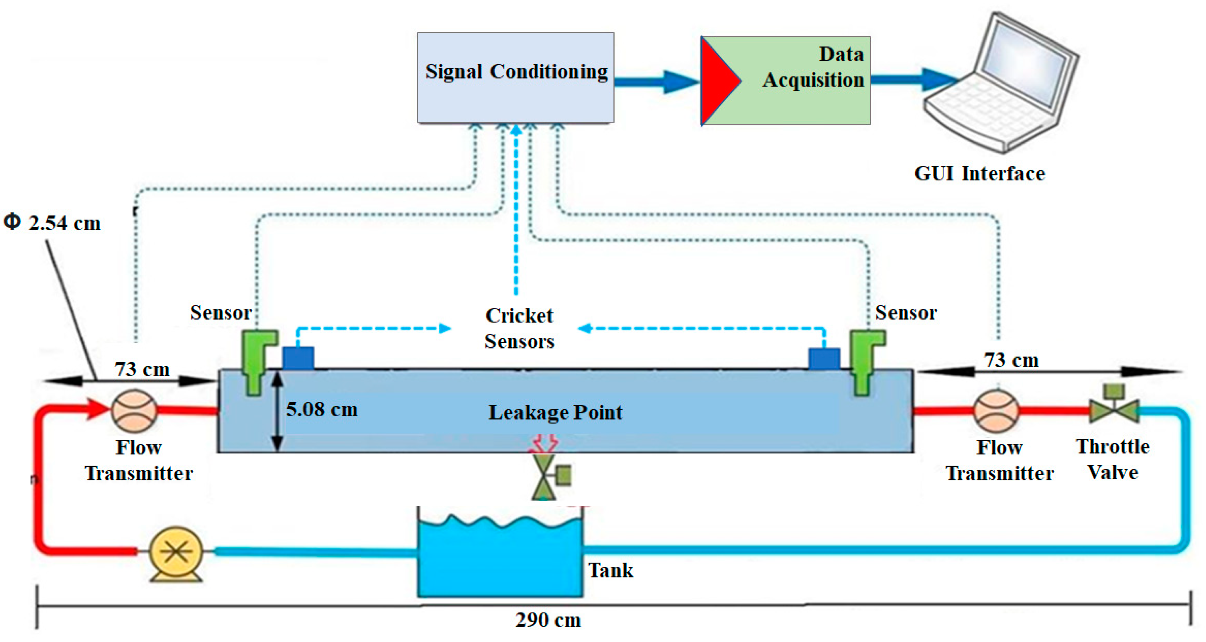
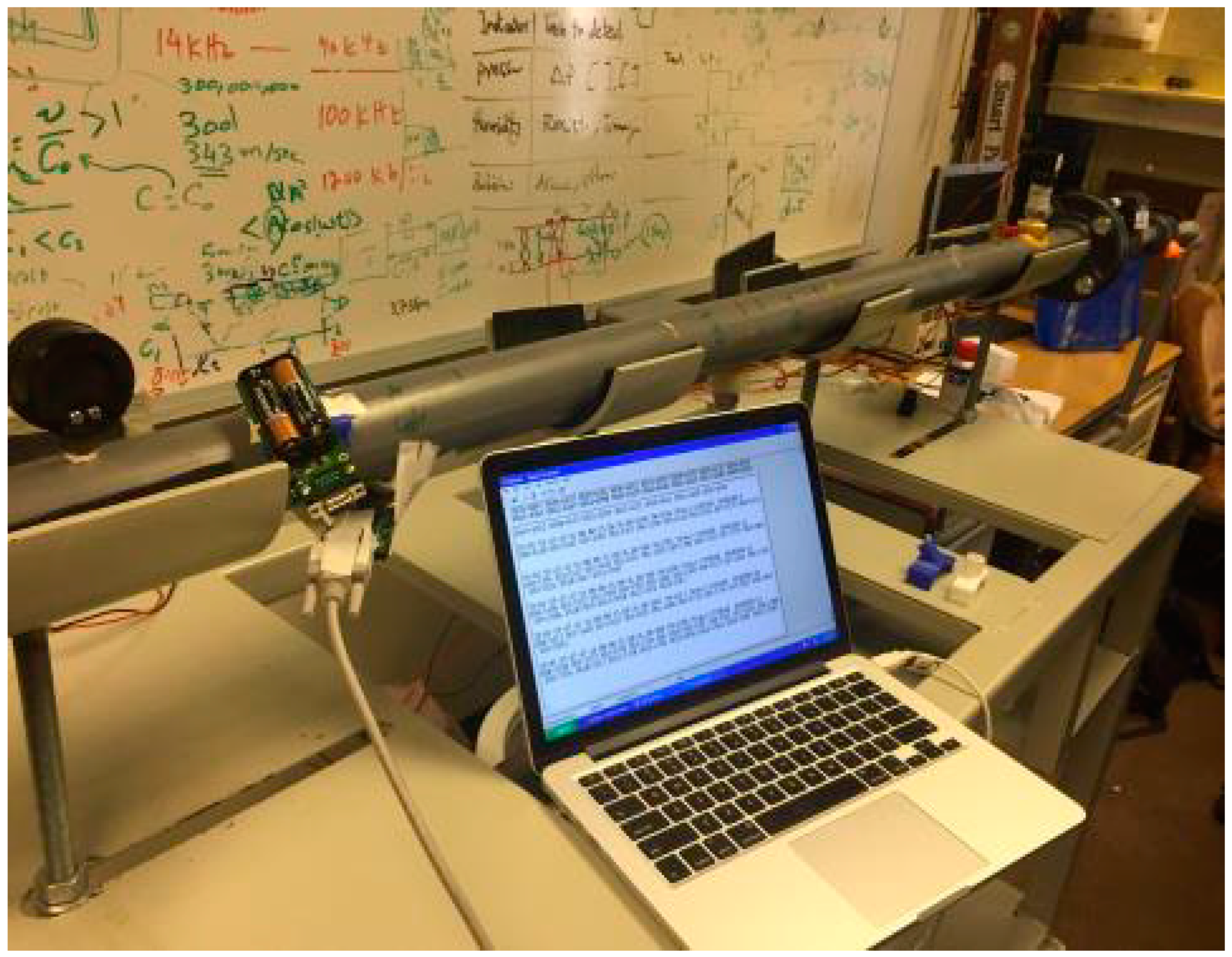
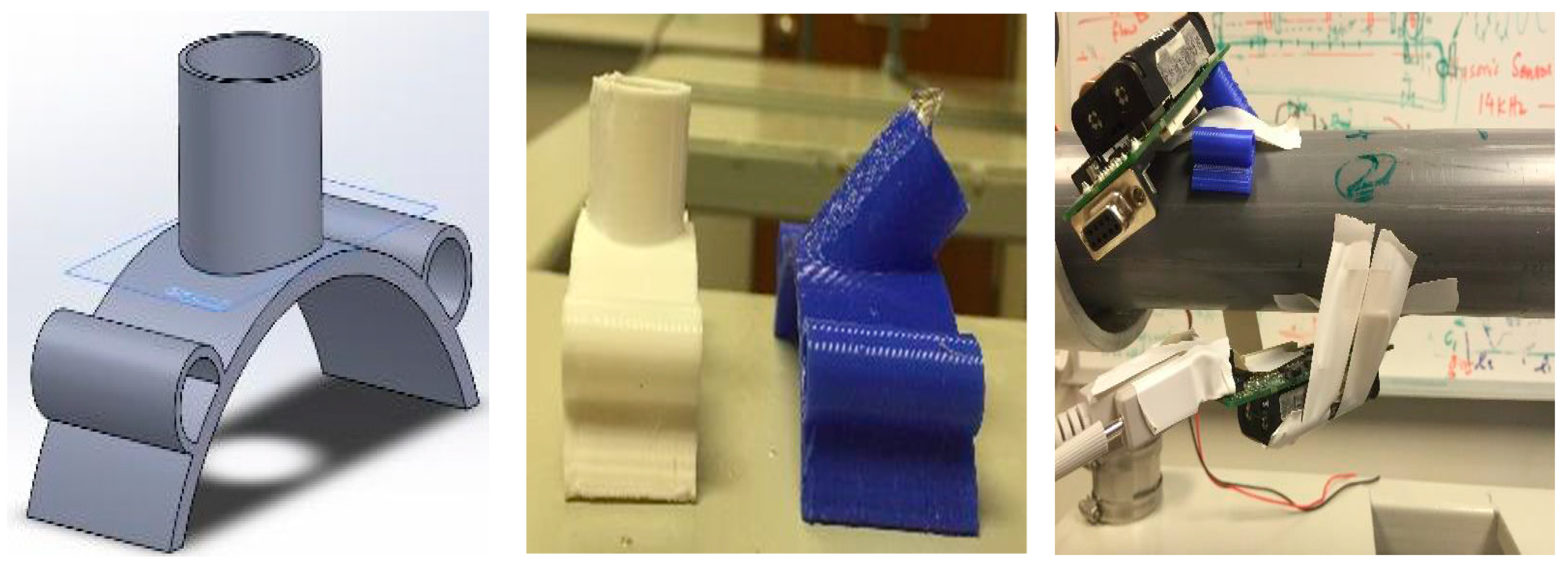
2.1. Experimental Setup

The experimental setup, shown in Figure 1 and Figure 2, is a closed-loop system. Starting at a reservoir tank, water is pumped into a PVC pipe that hosts a designed small leak and then returned to the same reservoir tank. The flow loop is equipped with metering valves that are designed to provide accurate and stable control of fluid flow rates. All recorded measurements are taken under a steady flow condition which is guaranteed by closing the throttle valve manually so that air trapped in the pipe is completely forced out through the pressure sensor vent. The throttle valve is opened after the sensor vent is closed as the flow becomes reasonably uniform. The measurements are taken from the middle pipe, which is 1.77 m long and has a diameter of 5.08 cm. An 88.5 cm distance is measured from the left end of the middle pipe, and a leaking valve is then slightly opened to resemble a tiny leak at the pipe wall. Thus, an early stage leaking pipe situation is studied using the two vital water flow characteristics of flow speed and fluid pressure that are measured at specific locations along the pipe. Five points, located at 50, 83, 89, 96, and 127 cm, measured from the left end of the middle pipe, are selected for measuring flow speed along the pipe.
In order to guarantee the preciseness of experimental measurements, sensor holders, as shown in Figure 3, are designed, along with 3D printed to hold the sensors accurately around the pipe. Two acoustic sensors (acting as a sender and a receiver) are used to find the flow’s speed. Couplet gel is used between the outer wall of the pipe to prevent ultrasonic wave leakage to surrounding air and ensure full coupling to the pipe. These acoustic sensors work by sending an ultrasonic wave that propagates through the pipe flow, as clarified in Figure 4. The acoustic signal is affected by any changes along the wave propagation path. In the case of changing the flow rate of the fluid, the signal time of propagation is altered. In order to measure fluid velocity, two time-of-propagation readings are taken; one is for a signal traveling with the flow, and the other is for a signal traveling in an opposite direction to the flow. The sensors are aligned in a suitable direction to capture the signals propagating with the flow and against it, [45]. The difference between the times of propagation for the two signals is correlated to the fluid velocity according (1)
V = [ ( T d T u ) / T d T u ) ] L 2 / 2 D
where V is the flow velocity, Td is the time of the wave propagating with the flow, and Tu is the time of the wave propagating against the flow. For accurate measurement of the distance (L) between ultrasonic transducers (T), two Cricket (40 kHz) sensors, which work on a combination of radiofrequency and ultrasonic technologies, are used. As depicted in Figure 4, D is Lcosɵ or Lsinɵ. The equipment used for measuring the velocity of flow is designed by “MEMSIC Transducer Systems”.
To measure levels of pressure drop due to fluid leakage, two pressure transducers are employed, one at an upstream location before the leaking point and one at a downstream location after the leaking point. The pressure transducers can measure up to 16 × 105 Pa, although they can withstand up to 25 × 105 Pa. The pressure transducers are also used to make sure that the fluid flow in the pipe is steady.
Flow rates are also measured. The testbed includes two fixed ultrasonic flow meters, which have a 60–200 × 103 cm3/min measuring range and can operate at a pressure value up to 16 × 105 Pa. To evaluate the amount of water being leaked, the inlet flow and the outlet flow are compared. A non-zero difference in the volumetric flow rate indicates the presence of a leak between ultrasonic fluid flow meters. To measure the amount of water leaked, a comparison between the inlet flow and the outlet flow in terms of volumetric flow rate, as apparent in (2)
Q = V A
where Q is the flow rate (cm3/s), V is the flow velocity (cm/s), and A is the cross-sectional pipe area (cm2). Since the cross-sectional area along the pipe is constant, it is sufficient to measure the values of velocity along the pipe rather than the flow rate since velocities can be easily measured at different locations along the pipe using ultrasonic sensors. Thus, the fluid flow rate can be evaluated by two measurements taken at the inlet and outlet of the middle pipe.
LabVIEW software is used to collect data from pressure transducers and fluid flow meters. The analog signals that arise from the flow meter and are generated by the pressure transducer require signal conditioning before digitization. For example, the amplification of the voltage levels of signals from the pressure transducer is required for better data acquisition. The data acquisition (DAQ) unit is used for digitizing measured analog signals before they are fed into the computer for processing. The whole unit can be used for visualization, processing, and storing the measured data. The leaking valve is set to allow the flow rates shown in Table 1.

2.2. Numerical Model

COMSOL Multiphysics® is used to analyze fluid velocity distribution inside the pipe. The values of velocities are close to the wall where the Laminar and the Turbulent velocities have close magnitudes [46], as shown in Figure 5. The difference between the Laminar and Turbulent velocities is highest in the middle of the pipe. The Reynolds number for used experimental conditions, which indicates turbulent flow, was calculated. Turbulent flow, K-ϵ, from the COMSOL Multiphysics is considered to analyze the flow in a pipe. K-ϵ supports both compressible and incompressible flows. The continuity equation and Navier-‘Stokes’ equations (for conservation of mass and conservation of momentum) are the equations that are being solved by K-ϵ. Three boundary conditions (velocity inlet 1, velocity outlet 2, and pressure outlet 3) are used in the simulation. The inlet of the pipe is referred to as “velocity inlet 1”. The outlet of the pipe is referred to as “pressure outlet 3”. The leak point is referred to as “velocity outlet 2”. Values assigned in different cases to these conditions are given in Table 1.

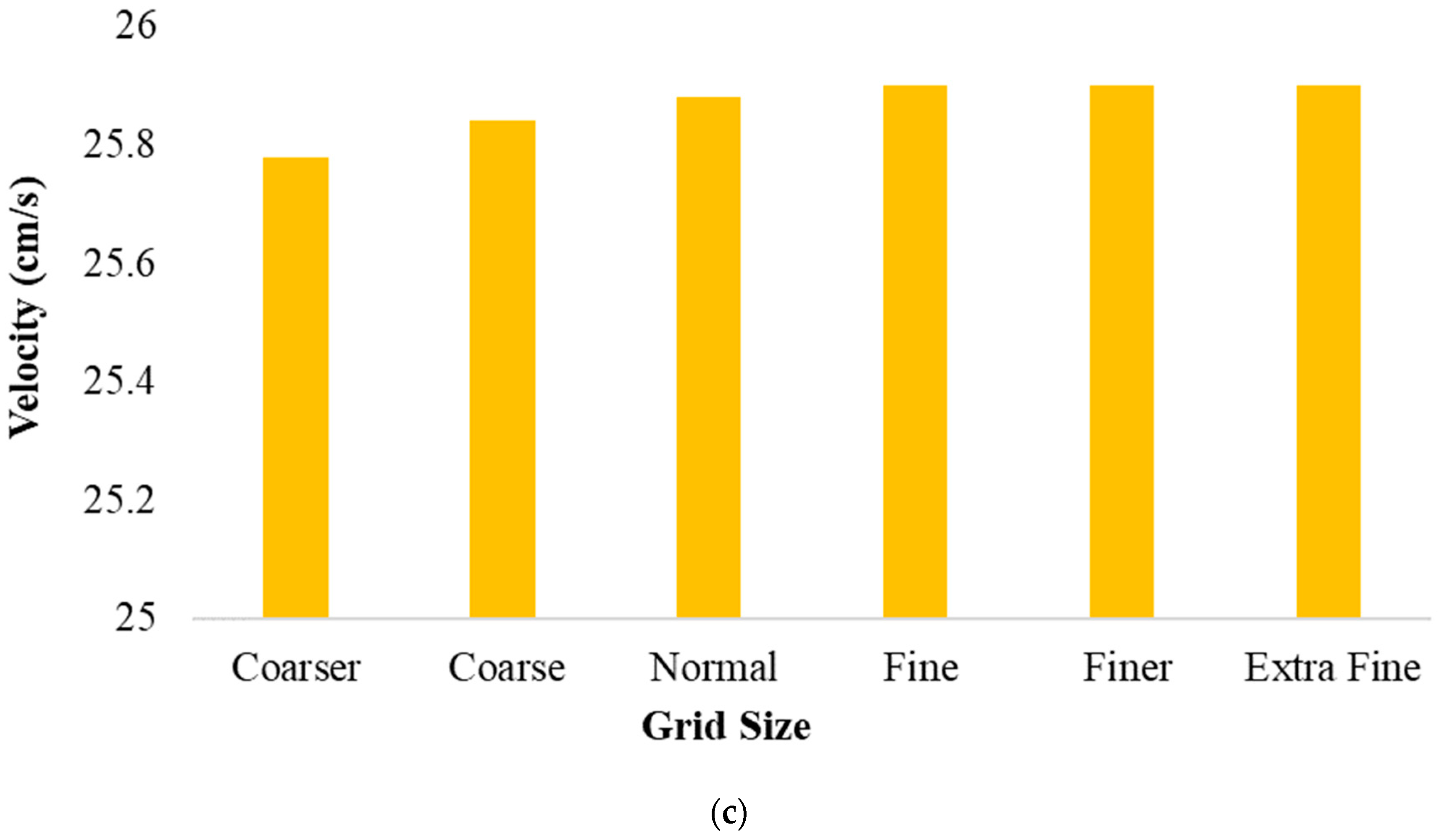
Geometry and Mesh Creation

The analysis is performed on a pipe that is 5.08 cm in internal diameter and 177 cm in length. A leak in the shape of a circular hole is used in the simulation. The leak has an area equal to that of the leak valve used in the experimental testbed. After selecting the Laminar Flow Model, the pipe geometry is created in the geometry section of the model component.
A Free Tetrahedral node is selected to create an unstructured tetrahedral mesh, as shown in Figure 6a. A finer mesh is created around the leaking hole at the pipe wall, as shown in Figure 6b, whereas for a smooth transition, the fine mesh is selected along the main pipe.
A powerful feature in COMSOL is that one can control the number, size, and distribution of elements by using size and distribution sub-nodes. The mesh density is kept nearly consistent to ensure the uniformity of obtained results. The grid dependency study is performed, as shown in Figure 6c. For mesh dependency, coarser mesh (4103 elements, & minimum element size of 4.96 cm), coarse mesh (6115 elements, & minimum element size of 4.05 cm), normal mesh (9059 elements, & minimum element size of 3.19 cm), fine mesh (31,090 elements, & minimum element size of 1.77 cm), finer mesh (244,304 elements, & minimum element size of 0.708 cm), and extra fine mesh (625,959 elements, & minimum element size of 0.266 cm) were considered. The solution becomes almost constant as the grid density is increased beyond the fine grid size.

3. Analysis & Results

In this section, the numerical simulations and the experiments are presented and analyzed in detail.

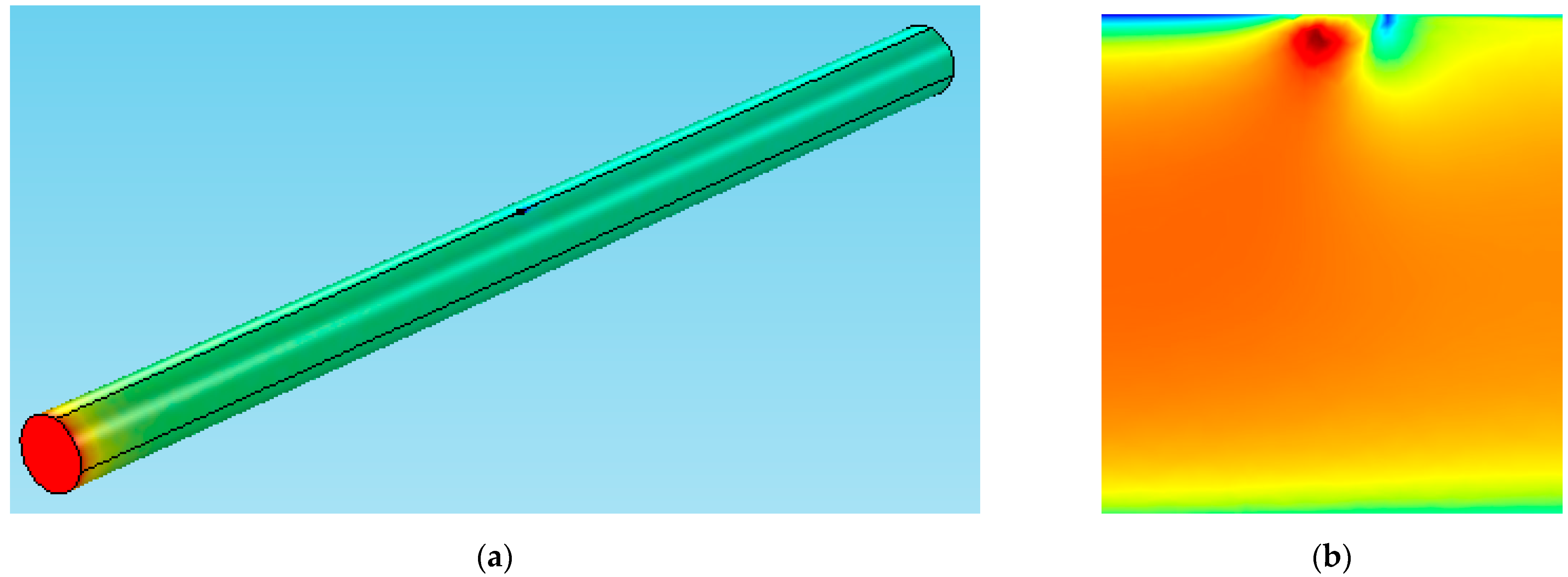
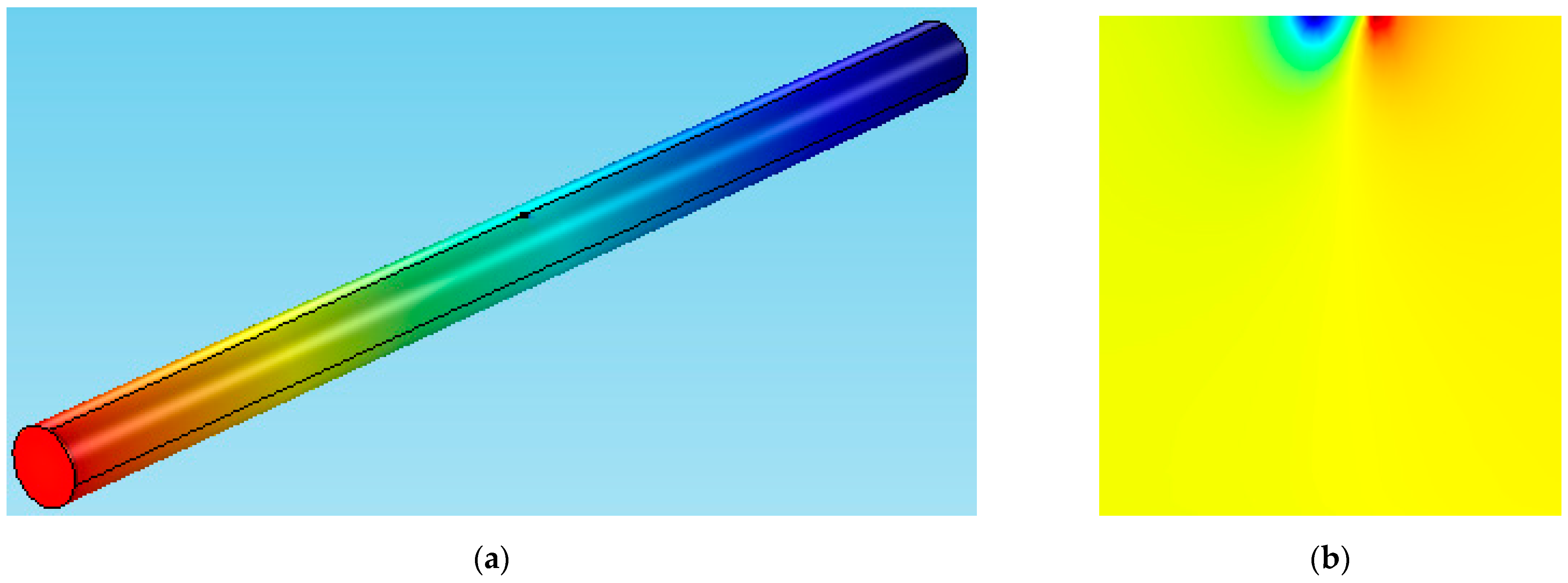
3.1. Numerical Simulations

Figure 7 and Figure 8 show the velocity and pressure contours in the vicinity of the leak (bottom center of the pipe) point in both longitudinal and transverse directions for the case of the mass flow rate of 3 cm3/s through the leaking valve.
The magnitude of the velocity is clearly at its maximum at the center of the pipe and minimum at the vicinity of the pipe wall due to drag viscous forces acting on the fluid near the wall, as shown in Figure 7. Moreover, the magnitude of pressure is observed to be higher in the downstream rather than the upstream due to pressure reduction induced by the leak formed in the middle section of the pipe, as shown in Figure 8.

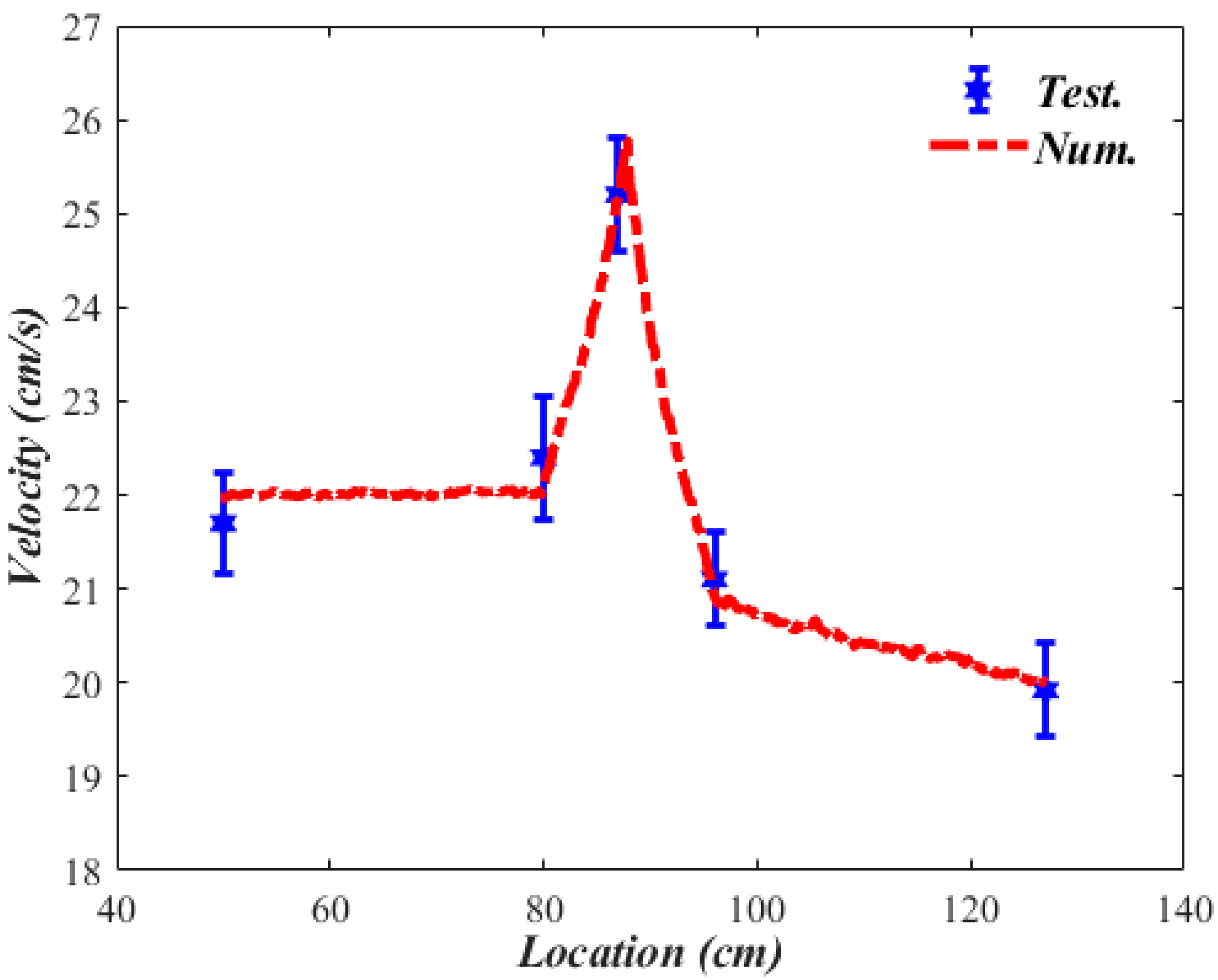
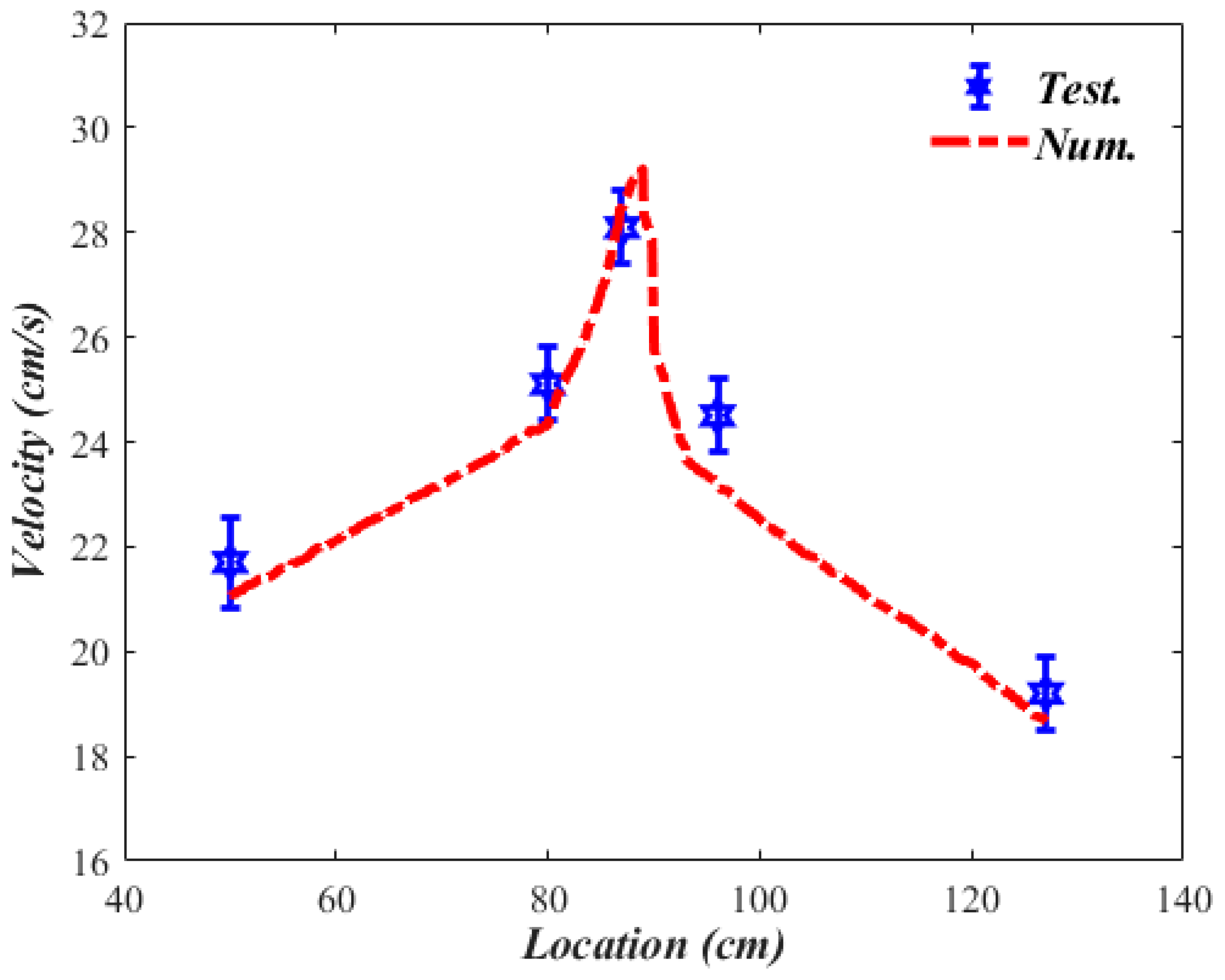
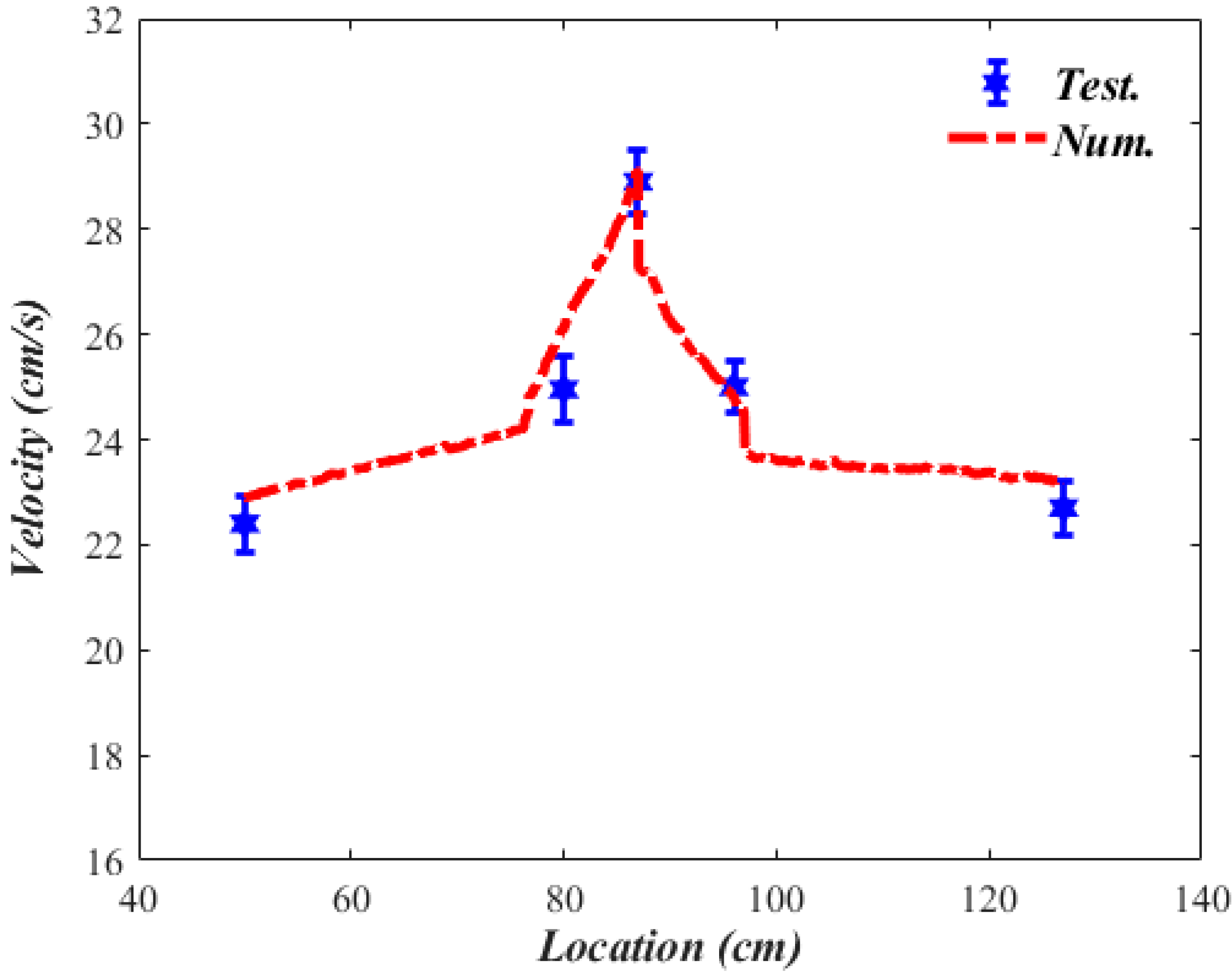
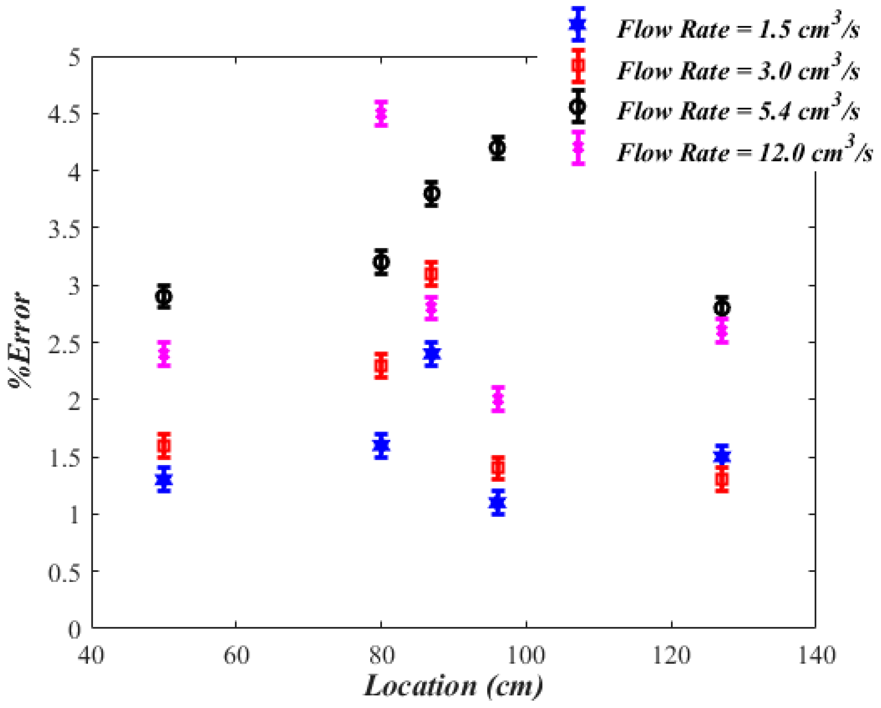
3.2. Comparisons between Experimental Results & Numerical Simulations

The results obtained from the experiments are compared with those obtained from analyses performed in COMSOL. The fluid velocity variation rates along the leaking pipes obtained experimentally and numerically are shown in Figure 9, Figure 10, Figure 11 and Figure 12. Each figure shows the fluid velocity variation for a pipe with leaks of different sizes.
Figure 9 compares experimentally measured and numerically calculated fluid velocity along a defective pipe with a leaking crack that has a mass flow rate of 1.5 cm3/s. A nearly constant velocity magnitude is observed before and after the leak location due to mass conservation. At the center of the pipe, where the leak is located, an experimental peak value of 25.5 cm/s and a numerical peak value of 24.8 cm/s are observed.
Experimental measurements and the numerical solutions are repeated on the same pipe with different leak sizes, as shown in Figure 10, Figure 11 and Figure 12. From these figures, it can be deduced that as one moves along the pipe, there is a sudden fluctuation in the flow velocity magnitude around the leak location; this is common for all leak sizes. A comparison between numerical and experimental results exhibits a similar trend in the flow velocity profile in all cases of differing leak sizes. Results for values at the selected points along the pipe are summarized in Table 2.
Considering the experimental measurements (EM) of the flow velocity as reference values, the percentage errors between experimental measurements (EM) and numerically calculated (NC) values are calculated using % E r r o r = [ ( E M N C ) E M ] × 100 and plotted in Figure 13.
For all cases of different leak sizes, it is observed that the % error is small, ranging between 1.0 and 5.0% at upstream locations far from the leaking point, i.e., at the 50 cm and 83 cm locations on the pipe. At locations close to the leak, i.e., 89 cm and 96 cm, the % error is slightly more. It is noted that bigger % errors are associated with larger sized leaks. For leak flow rate of 1.5 cm3/s, the % error at 89 cm is 2.3%, whereas at the same location, a % error of 2.9% can be seen for the leak flow rate of 12 cm3/s. At downstream locations far from the leak, the % error is small, ranging between 1.0 and 3.0%. The magnitude of error can be linked to the fact that leaking cracks causes eddies/instabilities to form in the flow field, which affects velocity measurements and, in turn leads to a higher level of measurement errors.
Having established a physically sound comparison between experimental measurements and numerical results, one can move to consider the effect of leaking crack geometry on the flow field inside the pipe. Ultimately, the motivation of the numerical simulations is to have a link between the root cause of the leak and the measurements taken from the flow field. This can be significantly valuable for characterizing the leaks that are difficult to bring under direct visibility, such as leaks in buried pipes.

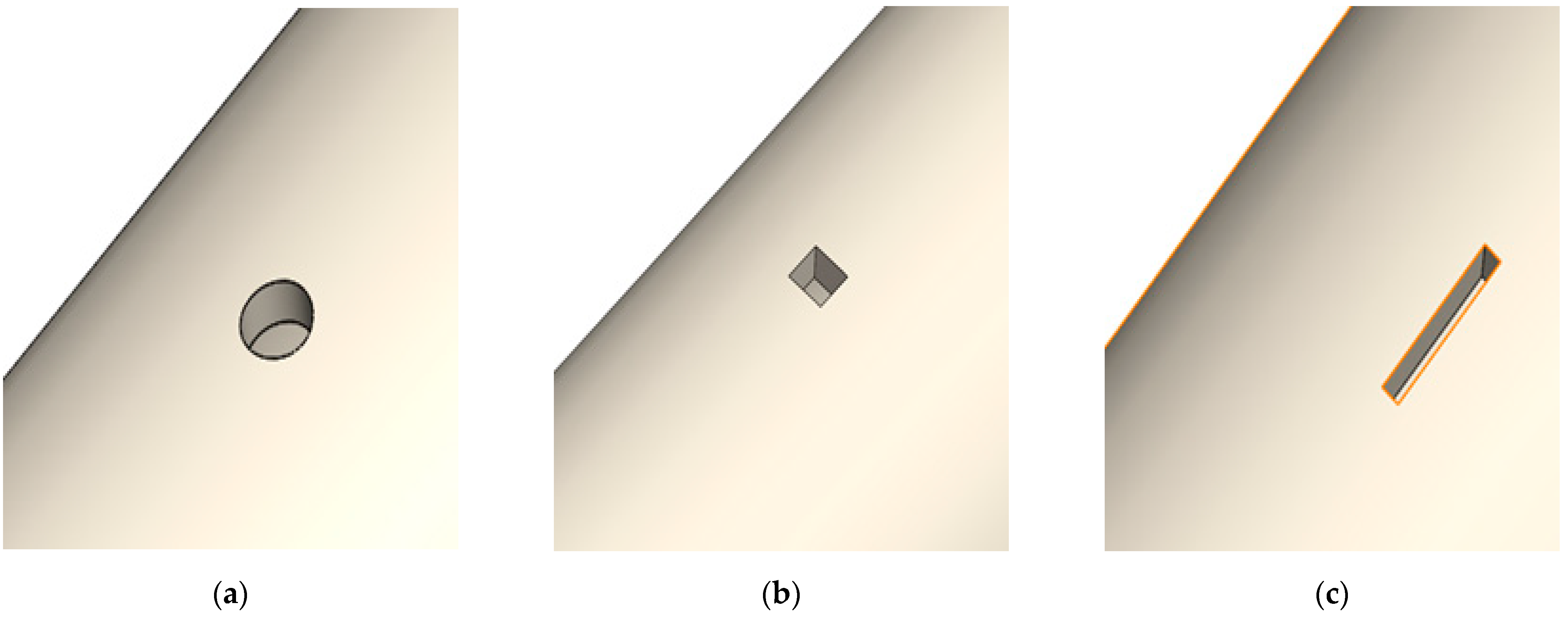
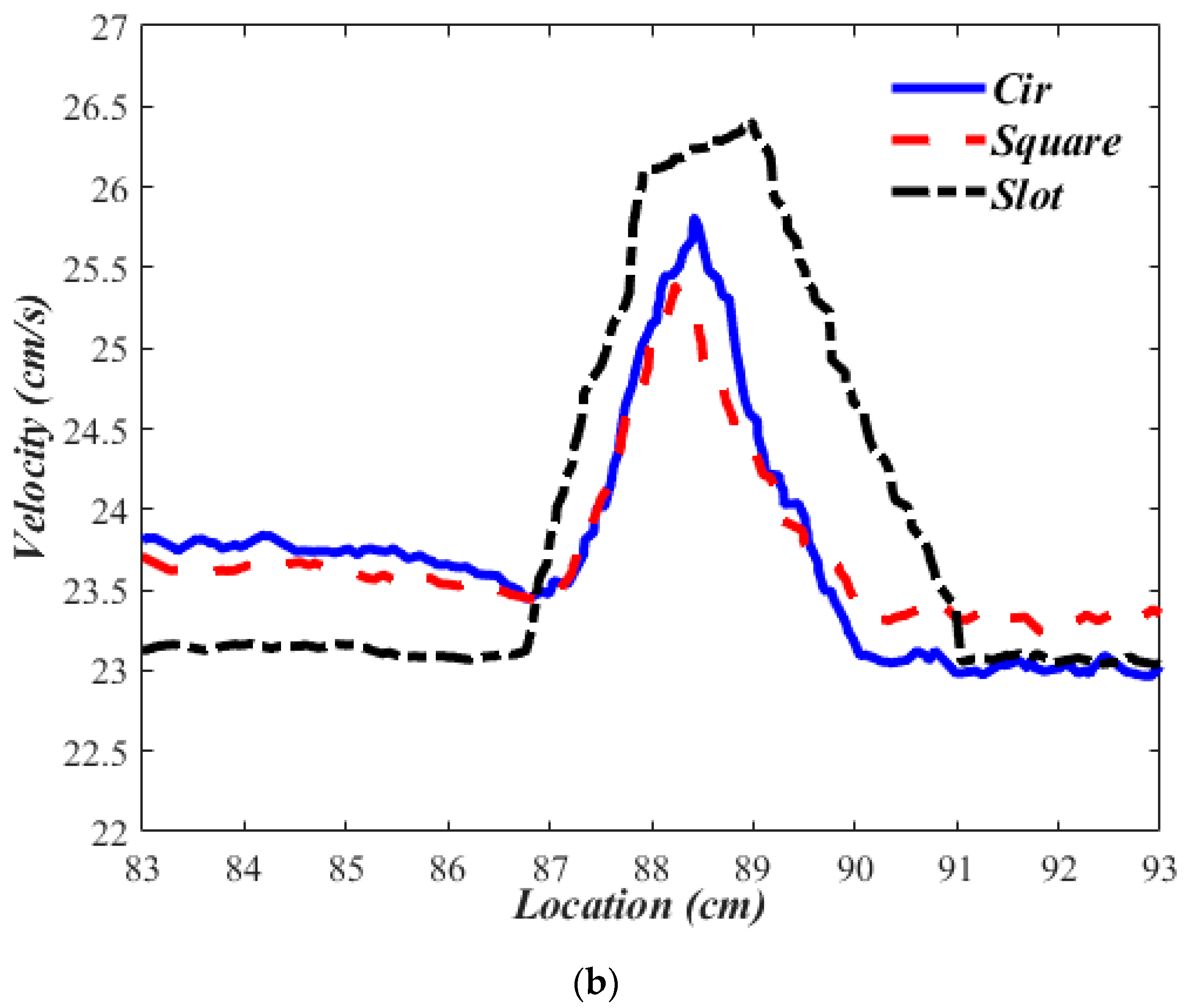
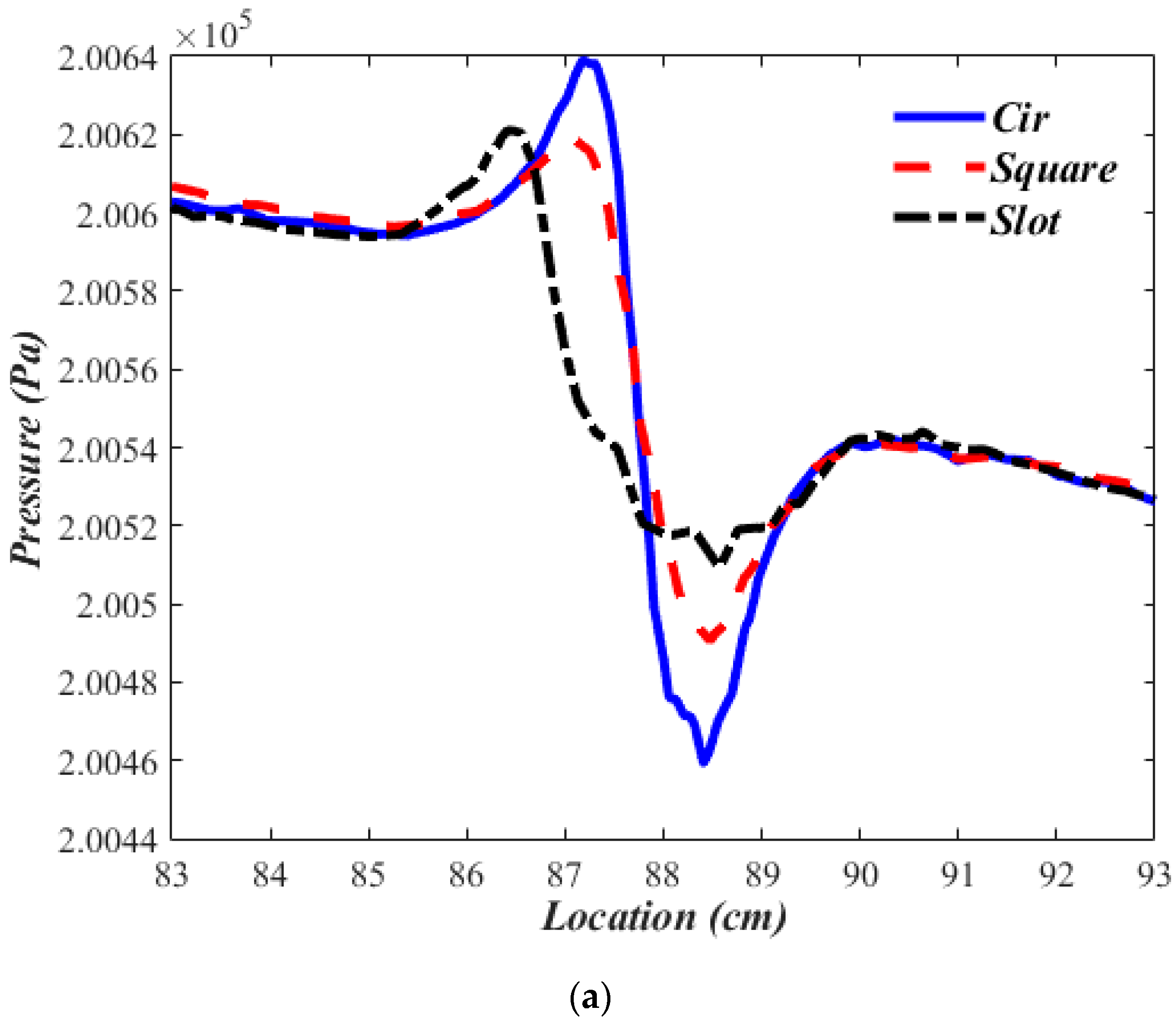
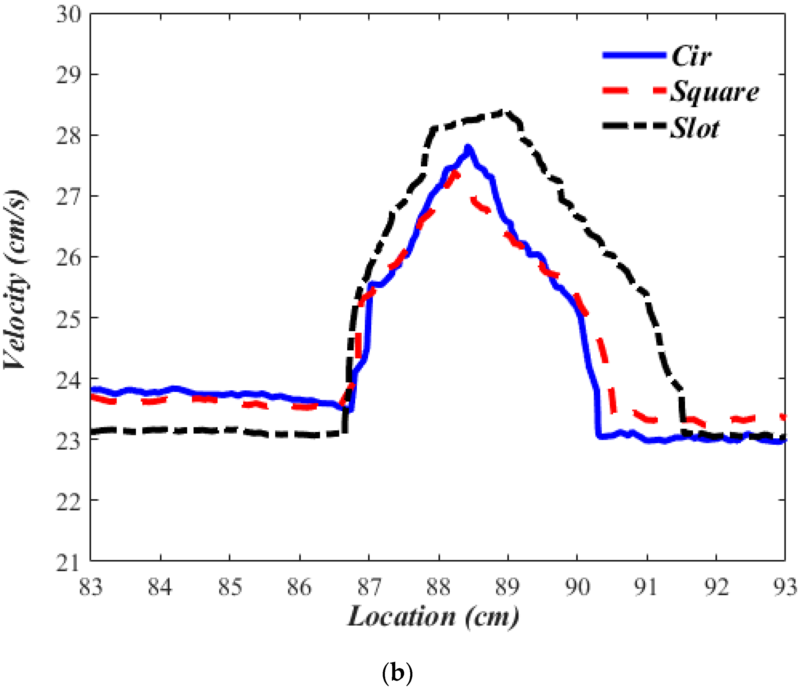
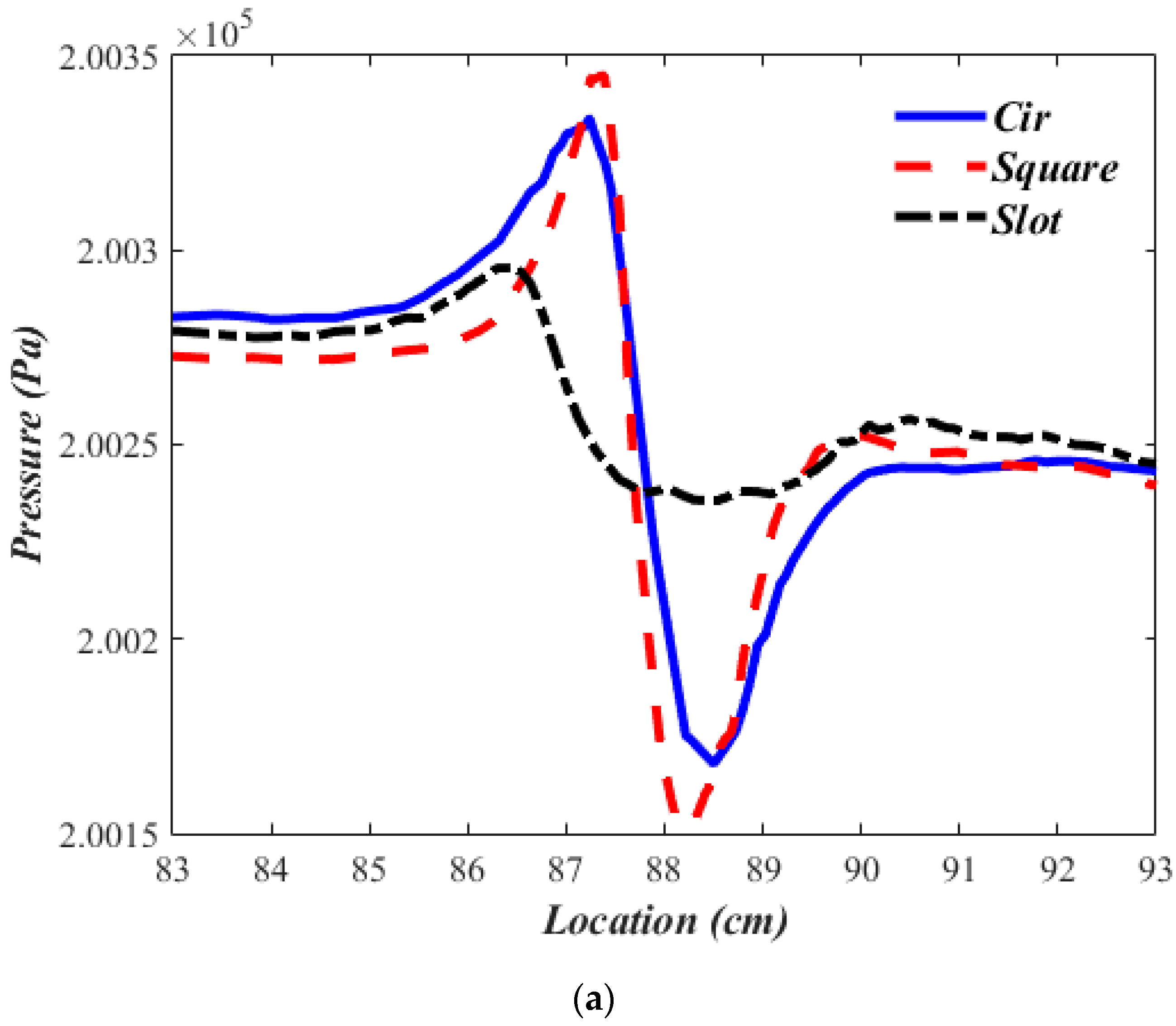
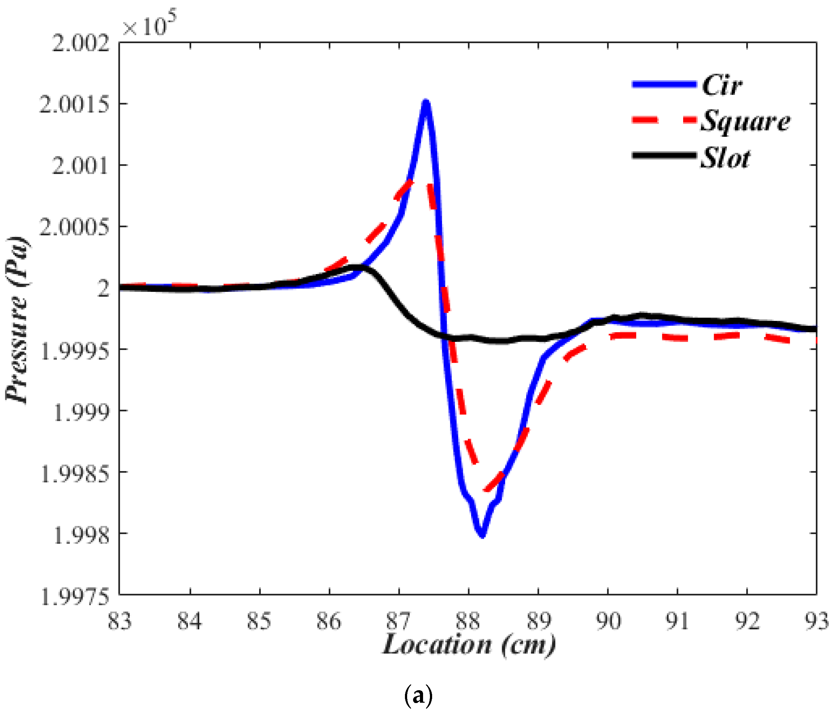
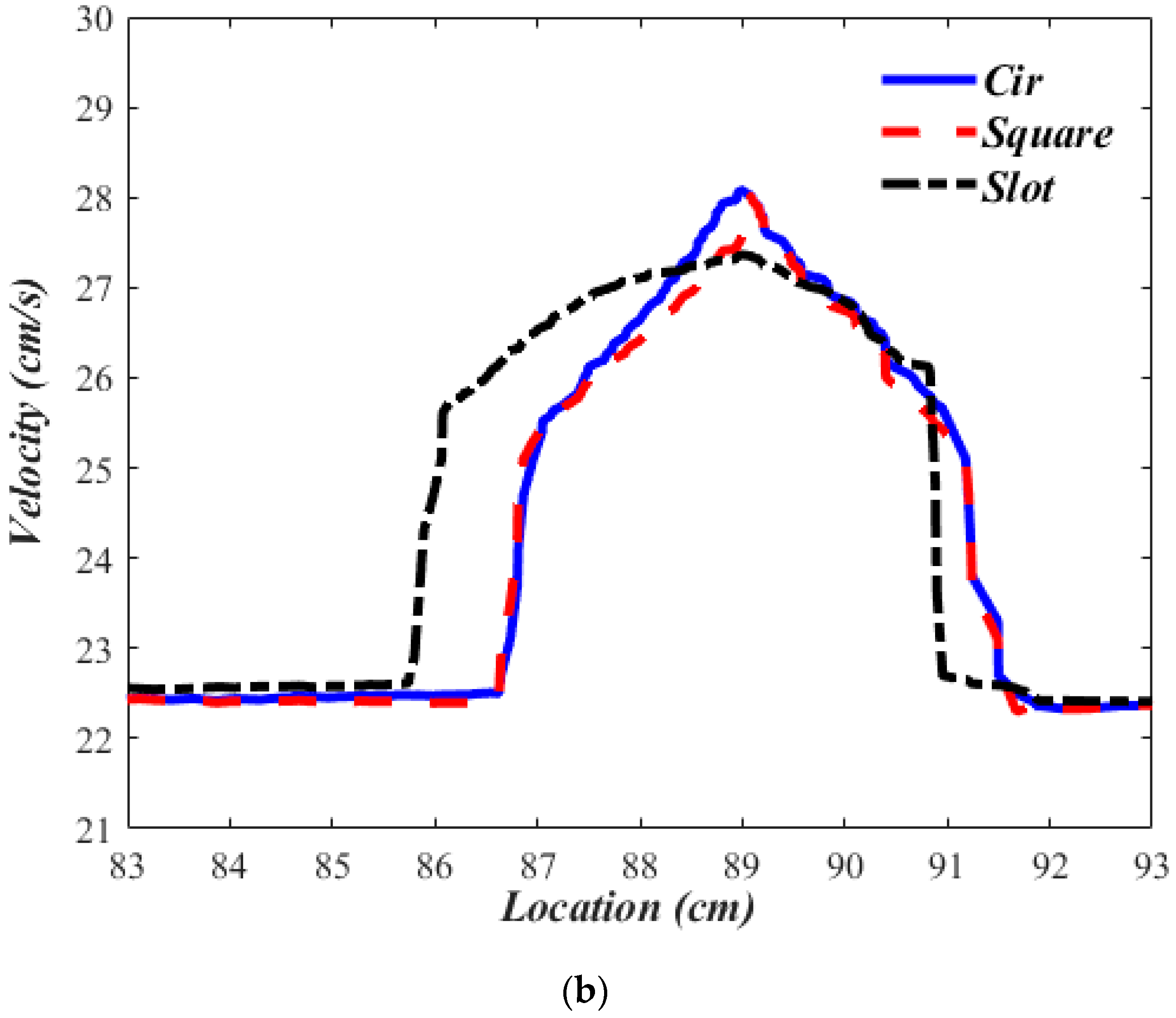
3.3. Pipe Geometry, Crack Geometry & Flow Conditions

Numerical analysis is now performed on two pipes of different sizes that have different flow conditions. Each pipe is assumed to have a leak that has one of three different geometries: a circle-shaped crack, a square-shaped crack, and a slot-shaped crack, as apparent in Figure 14. The numerical simulation can accommodate cracks that are more complex in shape, which also includes irregularly shaped cracks. However, understanding the influence of basic shaped cracks on the fluid flow characteristics is the focus of this paper. Thus, numerical analyses are performed to understand the influence of each crack geometry on pressure and velocity variations along the pipe, assuming that all cracks have the same area of 0.81 cm2. Table 3 shows the dimensions of the two pipes under study, and Table 4 shows the fluid flow conditions in each pipe. Table 5 shows the dimensions of the cracks formed at the walls of the pipes.
As previously mentioned, leaks can be caused by different factors. As a result, leaks can have different geometries. For example, a leak caused by excessive pressure has a different geometry from a leak caused by corrosion. This calls for creating an expert system that links leak geometry to its cause. Since such an expert system does not exist yet, we would like to study three different representative leak geometries, including circular, square, and slot-shaped cracks, and investigate the effect of these cracks on the flow inside a pipe. This will hopefully direct attention towards identifying the causes of the leak by measuring flow characteristics inside a pipe, which would form a cheap, efficient, and non-destructive way of evaluating pipelines.
A comparative study is performed on pressure and velocity distributions along two pipes of different sizes, that are carrying different fluid flows, and hosting leaks with different geometries, as shown in Figure 15, Figure 16, Figure 17 and Figure 18. In all figures, it is observed that the pressure varies rapidly while the velocity is highest in the vicinity of the leaking crack.
In the smaller sized pipe which has a diameter of 5.08 cm, the pressure causes a rise to a maximum value just before the leak, then rapidly dips to a minimum value at the leaking point and returns to its nominal value after the leak. Pressure fluctuations in the vicinity of leak are summarized Table 6. Both the largest and smallest pressure fluctuations occur in case of the circular crack.
The velocity variation around the leak location is characterized by an increase in value where the velocity has a maximum value, as is the case for square and circular leaks. Interestingly the velocity distribution around the leak has a number of peak values, as is the case for the slotted-crack shape. Velocity variations in the vicinity of leak are summarized Table 6.
A similar trend in the pressure and velocity gradient at the leakage locality is observed for flow condition-2 (0.0005 m3/s flow rate & 20 × 103 Pa pressure) conditions with, Figure 17 and Figure 18.
As for the effect of leaks with different shapes on the pipe flow characteristics, one can observe that pressure and velocity fluctuations induced by the circular and square-shaped cracks follow a similar trend with a difference in peak values. On the other hand, the pressure and velocity fluctuations induced by the slot-shaped crack are well distinguished from those induced by circular and square-shaped cracks, based on numerical simulation results. Therefore, if one is able to obtain information regarding the pressure/velocity distribution along a cracked (leaking) pipe, it is then possible to predict the shape and size of the leak. Predicting the geometry of a leak could lead to identifying the cause of the crack and proposing an effective remedy for fluid leak control. The effect of the leakage size is also investigated. For circular shapes, three different radii (0.708 cm, 0.508 cm, and 0.308 cm) were considered.
Pressure and velocity variations along pipe length for cases in which a circular shaped leak has three different leak radii are shown in Figure 19. One can observe that pressure and velocity fluctuations follow a similar trend with a difference in peak values. The effect of the aperture size (leak radius) is more significant in the pressure measurement as compared to the velocity measurement.

4. Conclusions

Experimental and numerical investigations have been carried out to discover the effect of the geometry of a leaking crack on fluid flow characteristics inside water pipes. The influence of a circular shaped crack, drilled through a pipe wall, on the velocity and pressure measured distributions was compared with a COMSOL simulated pipe with a similar leakage. The experimentally measured and numerically calculated velocity distributions along a water pipe were found to agree well in the general trends of increasing/decreasing velocity values around a leak location. The value of the magnitude of pressure was observed to be higher in the upstream than the downstream due to pressure disturbance caused by the leak. Then, CFD numerical investigations were conducted on cracks with different shapes, including those with slot, circle, and square-shaped geometries. The turbulent fluid flow models showed that the variation of pressure and velocity distributions in the vicinity of the leak locations were found to be influenced by the crack geometry. The pressure and velocity fluctuations induced by circular and square-shaped cracks were found to follow similar trends but were different from those brought in by the slot-shaped crack. The influence of the leak size was also numerically investigated. Pressure and velocity variations along pipe length for cases with a circular shaped leak that had three different leak radii were found to follow a similar trend though there was a difference in peak values. While this study is not exhaustive enough to consider leaks with several geometrical configurations, it clearly indicates that crack geometry could be predicted from the measurement of pressure/velocity distribution along the pipeline. This paper calls for conducting extensive experimental and numerical studies with a focus on data analysis. In particular, predictive artificial intelligence mechanisms should be employed to understand the relationships between flow characteristics and leak geometries on one level, as well as the connection of each crack geometry to its root cause at a higher level.

Author Contributions

Conceptualization, U.B. and M.A.H.; methodology, S.A., U.B. and M.A.H.; software, S.A.; validation, S.A. and M.A.H.; formal analysis, S.A. and M.A.H.; investigation, U.B. and M.A.H.; resources, U.B. and M.A.H.; data curation, S.A. and M.A.H.; writing—original draft preparation, S.A.; writing—review and editing, S.A., U.B. and M.A.H.; visualization, S.A.; supervision, U.B. and M.A.H.; project administration, U.B. and M.A.H.; funding acquisition, U.B. All authors have read and agreed to the published version of the manuscript.

Funding

This research was funded by the King Abdulaziz City for Science and Technology (KACST) through King Fahd University of Petroleum & Minerals (KFUPM) via Project No. 12-ELE2381-04) as part of the National Science, Technology and Innovation Plan.

Institutional Review Board Statement

Not applicable.

Informed Consent Statement

Not applicable.

Data Availability Statement

The data that support the findings of this study are available on request from the corresponding author. The data are not publicly available due to privacy or ethical restrictions.

Acknowledgments

The authors would like to acknowledge and appreciate the support provided by the Deanship of Scientific Research (DSR) at King Fahd University of Petroleum & Minerals (KFUPM) for conducting this research.

Conflicts of Interest

The authors declare no conflict of interest.

References

  1. Da Silva, H.V.; Morooka, C.K.; Guilherme, I.R.; da Fonseca, T.C.; Mendes, J.R.P. Leak detection in petroleum pipelines using a fuzzy system. J. Pet. Sci. Eng. 2005, 49, 223–238. [Google Scholar] [CrossRef]
  2. Ishido, Y.; Takahashi, S. A new indicator for real-time leak detection in water distribution networks: Design and simulation validation. Procedia Eng. 2014, 89, 411–417. [Google Scholar] [CrossRef] [Green Version]
  3. Martini, A.; Troncossi, M.; Rivola, A. Vibration Monitoring as a Tool for Leak Detection in Water Distribution Networks. In Proceedings of the International Conference Surveillance 7, Chartres, France, 29–30 October 2013. [Google Scholar]
  4. Baroudi, U.; Al-Roubaiey, A.A.; Devendiran, A. Pipeline Leak Detection Systems and Data Fusion: A Survey. IEEE Access 2019, 7, 97426–97439. [Google Scholar] [CrossRef]
  5. El-Zahab, S.; Zayed, T. Leak detection in water distribution networks: An introductory overview. Smart Water 2019, 4, 5. [Google Scholar] [CrossRef] [Green Version]
  6. Liston, D.A.; Liston, J.D. Leak detection techniques. J. N. Engl. Water Work. Assoc. 1992, 106, 103–108. [Google Scholar]
  7. Hunaidi, O. Detecting Leaks in Water-Distribution Pipes. Inst. Res. Constr. 2000, 40, 1–6. [Google Scholar]
  8. Puust, R.; Kapelan, Z.; Savic, D.A.; Koppel, T. A review of methods for leakage management in pipe networks. Urban Water J. 2010, 7, 25–45. [Google Scholar] [CrossRef]
  9. Ayala-Cabrera, D.; Herrera, M.; Izquierdo, J.; Ocaña-Levario, S.J.; Pérez-García, R. GPR-based water leak models in water distribution systems. Sensors 2013, 13, 15912–15936. [Google Scholar] [CrossRef]
  10. Navarro, A.; Begovich, O.; Sanchez-Torres, J.D.; Besancon, G.; Murillo, J.A.P. Leak detection and isolation using an observer based on robust sliding mode differentiators. In Proceedings of the World Automation Congress Proceedings, Puerto Vallarta, Mexico, 24–28 June 2012. [Google Scholar]
  11. Torres, L.; Besançon, G.; Navarro, A.; Begovich, O.; Georges, D. Examples of pipeline monitoring with nonlinear observers and real-data validation. In Proceedings of the 8th International Multi-Conference on Systems, Signals & Devices, Sousse, Tunisia, 22–25 March 2011; pp. 1–6. [Google Scholar]
  12. Liu, Z.; Kleiner, Y. State of the art review of inspection technologies for condition assessment of water pipes. Meas. J. Int. Meas. Confed. 2013, 46, 1–15. [Google Scholar] [CrossRef] [Green Version]
  13. Cataldo, A.; Cannazza, G.; De Benedetto, E.; Giaquinto, N. A new method for detecting leaks in underground water pipelines. IEEE Sens. J. 2012, 12, 1660–1667. [Google Scholar] [CrossRef]
  14. Choi, J.; Shin, J.; Song, C.; Han, S.; Park, D., II. Leak detection and location of water pipes using vibration sensors and modified ML prefilter. Sensors 2017, 17, 2104. [Google Scholar] [CrossRef] [PubMed] [Green Version]
  15. Bentoumi, M.; Chikouche, D.; Mezache, A.; Bakhti, H. Wavelet DT method for water leak-detection using a vibration sensor: An experimental analysis. IET Signal Process. 2017, 11, 396–405. [Google Scholar] [CrossRef]
  16. Asada, Y.; Kimura, M.; Azechi, I.; Iida, T.; Kubo, N. Transient damping method for narrowing down leak location in pressurized pipelines. Hydrol. Res. Lett. 2020, 14, 41–47. [Google Scholar] [CrossRef] [Green Version]
  17. Zhang, Y.; Chen, S.; Li, J.; Jin, S. Leak detection monitoring system of long distance oil pipeline based on dynamic pressure transmitter. Meas. J. Int. Meas. Confed. 2014, 49, 382–389. [Google Scholar] [CrossRef]
  18. Chatzigeorgiou, D.; Youcef-Toumi, K.; Ben-Mansour, R. Design of a novel in-pipe reliable leak detector. IEEE/ASME Trans. Mechatronics 2015, 20, 824–833. [Google Scholar] [CrossRef] [Green Version]
  19. Liu, C.W.; Li, Y.X.; Yan, Y.K.; Fu, J.T.; Zhang, Y.Q. A new leak location method based on leakage acoustic waves for oil and gas pipelines. J. Loss Prev. Process Ind. 2015, 35, 236–346. [Google Scholar] [CrossRef]
  20. Lang, X.; Li, P.; Cao, J.; Li, Y.; Ren, H. A small leak localization method for oil pipelines based on information fusion. IEEE Sens. J. 2018, 18, 6115–6122. [Google Scholar] [CrossRef]
  21. Lang, X.; Li, P.; Guo, Y.; Cao, J.; Lu, S. A multiple leaks’ localization method in a pipeline based on change in the sound velocity. IEEE Trans. Instrum. Meas. 2019, 69, 5010–5017. [Google Scholar] [CrossRef]
  22. Zeng, Y.; Luo, R. Numerical Analysis of Incompressible Flow Leakage in Short Pipes. In Proceedings of the 12th Pipeline Technology Conference, Berlin, Germany, 2–4 May 2017. [Google Scholar]
  23. Ali, S.; Kamran, M.A.; Khan, S. Effect of baffle size and orientation on lateral sloshing of partially filled containers: A numerical study. Eur. J. Comput. Mech. 2017, 26, 584–608. [Google Scholar] [CrossRef]
  24. Ali, S.; Khan, S.; Horoub, M.M.; Ali, S.; Albalasie, A.; Jamal, A. Effect of Baffles Location on the Rollover Stability of Partially Filled Road Container. In Proceedings of the 2020 2nd International Conference on Electrical, Communication, and Computer Engineering (ICECCE), Istanbul, Turkey, 12–13 June 2020; pp. 12–13. [Google Scholar] [CrossRef]
  25. Liu, C.; Li, Y.; Xu, M. An integrated detection and location model for leakages in liquid pipelines. J. Pet. Sci. Eng. 2019, 175, 852–867. [Google Scholar] [CrossRef]
  26. Zhang, Q.; Wu, F.; Yang, Z.; Li, G.; Zuo, J. Simulation of the transient characteristics of water pipeline leakage with different bending angles. Water 2019, 11, 1871. [Google Scholar] [CrossRef] [Green Version]
  27. He, J.; Yang, L.; Ma, Y.; Yang, D.; Li, A.; Huang, L.; Zhan, Y. Simulation and application of a detecting rapid response model for the leakage of flammable liquid storage tank. Process Saf. Environ. Prot. 2020, 141, 390–401. [Google Scholar] [CrossRef]
  28. Karney, B.; Khani, D.; Halfawy, M.; Hunaidi, O. A Simulation Study on Using Inverse Transient Analysis for Leak Detection in Water Distribution Networks. J. Water Manag. Model. 2009, 399–416. [Google Scholar] [CrossRef] [Green Version]
  29. Jang, S.P.; Cho, C.Y.; Nam, J.H.; Lim, S.H.; Shin, D.; Chung, T.Y. Numerical study on leakage detection and location in a simple gas pipeline branch using an array of pressure sensors. J. Mech. Sci. Technol. 2010, 24, 983–990. [Google Scholar] [CrossRef]
  30. Hosseinalipour, S.M.H.; Aghakhani, H. Numerical & experimental study of flow from a leaking buried pipe in an unsaturated porous media. World Acad. Sci. Eng. Technol. 2011, 5, 859–864. [Google Scholar] [CrossRef]
  31. De Sousa, J.V.N.; Sodré, C.H.; de Lima, A.G.B.; de Farias Neto, S.R. Numerical Analysis of Heavy Oil-Water Flow and Leak Detection in Vertical Pipeline. Adv. Chem. Eng. Sci. 2013, 3, 9–15. [Google Scholar] [CrossRef] [Green Version]
  32. Ben-Mansour, R.; Habib, M.A.; Khalifa, A.; Youcef-Toumi, K.; Chatzigeorgiou, D. Computational fluid dynamic simulation of small leaks in water pipelines for direct leak pressure transduction. Comput. Fluids 2012, 57, 110–123. [Google Scholar] [CrossRef]
  33. Guo, X.L.; Yang, K.L.; Li, F.T.; Wang, T.; Fu, H. Analysis of first transient pressure oscillation for leak detection in a single pipeline. J. Hydrodyn. 2012, 24, 363–370. [Google Scholar] [CrossRef]
  34. Olegario, F.; Seleghim, P. Model Development and Numerical Simulation for Detecting Pre-Existing Leaks in Liquid Pipeline. In Proceedings of the 22nd International Congress of Mechanical Engineering (COBEM 2013), Ribeirão Preto, Brazil, 3–7 November 2013; pp. 6906–6915. [Google Scholar]
  35. Meniconi, S.; Brunone, B.; Ferrante, M.; Massari, C. Numerical and experimental investigation of leaks in viscoelastic pressurized pipe flow. Drink. Water Eng. Sci. 2013, 6, 11–16. [Google Scholar] [CrossRef] [Green Version]
  36. Xanthos, S.S.; Agathokleous, A.; Gagatsis, A.; Kranioti, S.; Christodoulou, S.E. Experimental and Numerical Investigation of Water-Loss in Water Distribution Networks. In Proceedings of the 2014 Intelligent Distribution for Efficient and Affordable Supplies [Water IDEAS 2014], Bologna, Italy, 22–24 October 2014; Available online: https://www.researchgate.net/profile/Symeon-Christodoulou/publication/267214360 (accessed on 15 March 2022).
  37. Liu, C.; Li, Y.; Meng, L.; Wang, W.; Zhao, F.; Fu, J. Computational fluid dynamic simulation of pressure perturbations generation for gas pipelines leakage. Comput. Fluids 2015, 119, 213–223. [Google Scholar] [CrossRef]
  38. De Sousa, C.A.; Romero, O.J. Influence of oil leakage in the pressure and flow rate behaviors in pipeline. Lat. Am. J. Energy Res. 2017, 4, 17–29. [Google Scholar] [CrossRef] [Green Version]
  39. Abdulshaheed, A.; Mustapha, F.; Ghavamian, A. A pressure-based method for monitoring leaks in a pipe distribution system: A Review. Renew. Sustain. Energy Rev. 2017, 69, 902–911. [Google Scholar] [CrossRef]
  40. Fu, H.; Yang, L.; Liang, H.; Wang, S.; Ling, K. Diagnosis of the single leakage in the fluid pipeline through experimental study and CFD simulation. J. Pet. Sci. Eng. 2020, 193, 107437. [Google Scholar] [CrossRef]
  41. Lyu, S.; Wang, W.; Zhang, Y. Leakage position of pipeline on the underground diffusion of crude oil. IOP Conf. Ser. Earth Environ. Sci. 2019, 237, 32119. [Google Scholar] [CrossRef]
  42. Gong, J.; Lambert, M.F.; Zecchin, A.C.; Simpson, A.R. Experimental verification of pipeline frequency response extraction and leak detection using the inverse repeat signal. J. Hydraul. Res. 2016, 54, 210–219. [Google Scholar] [CrossRef] [Green Version]
  43. Duan, H.-F. Transient frequency response based leak detection in water supply pipeline systems with branched and looped junctions. J. Hydroinform. 2016, 19, 17–30. [Google Scholar] [CrossRef]
  44. Bohorquez, J.; Alexander, B.; Simpson, A.R.; Lambert, M.F. Leak Detection and Topology Identification in Pipelines Using Fluid Transients and Artificial Neural Networks. J. Water Resour. Plan. Manag. 2020, 146, 4020040. [Google Scholar] [CrossRef]
  45. Markey, B.; Yu, Y.; Ban, T.; Johal, G. Time-of-flight application for fluid flow measurement. Opt. Diagnostics Sens. IX 2009, 7186, 71860S. [Google Scholar] [CrossRef]
  46. Hadush, T. Flow in pipes. Fluid Mech. 2004, 1–25. [Google Scholar]
Figure 1. A Schematic of the experimental testbed.
Sustainability 14 05224 g001
Figure 2. Experimental testbed.
Sustainability 14 05224 g002
Figure 3. 3D printed ultrasonic sensor holders at a right angle and a 45° angle.
Sustainability 14 05224 g003
Figure 4. Working principle of acoustic sensors.
Sustainability 14 05224 g004
Figure 5. Laminar (left), and turbulent (right) velocity profiles.
Sustainability 14 05224 g005
Figure 6. (a) Entire meshed pipe, (b) Meshing near the leakage, & (c) Grid dependency.
Sustainability 14 05224 g006aSustainability 14 05224 g006b
Figure 7. (a) Velocity contours in the longitudinal direction along the pipe, and (b) near leak area.
Sustainability 14 05224 g007
Figure 8. (a) Pressure contours in a transverse direction to the pipe, and (b) near leak area.
Sustainability 14 05224 g008
Figure 9. Velocity magnitude comparison along the pipe (with leak flow of 1.5 cm3/s).
Sustainability 14 05224 g009
Figure 10. Velocity magnitude comparison along the pipe (with leak flow of 3 cm3/s).
Sustainability 14 05224 g010
Figure 11. Velocity magnitude comparison along the pipe (with leak flow of 5.4 cm3/s).
Sustainability 14 05224 g011
Figure 12. Velocity magnitude comparison along the pipe (with leak flow of 12 cm3/s).
Sustainability 14 05224 g012
Figure 13. Percentage of error between experimentally and numerically obtained speeds of flow along the pipe.
Sustainability 14 05224 g013
Figure 14. (a) Circle-shaped crack, (b) square-shaped crack, and (c) slot-shaped crack.
Sustainability 14 05224 g014
Figure 15. Pressure (a) and Velocity (b) distributions along the 5.08 cm diameter pipe, with flow condition 1.
Sustainability 14 05224 g015aSustainability 14 05224 g015b
Figure 16. Pressure (a) and Velocity (b) distributions along the 5.08 cm diameter pipe, with flow condition 2.
Sustainability 14 05224 g016aSustainability 14 05224 g016b
Figure 17. Pressure (a) and Velocity (b) distributions along the 10.16 cm diameter pipe, with flow condition 1.
Sustainability 14 05224 g017aSustainability 14 05224 g017b
Figure 18. Pressure (a) and Velocity (b) distributions along the 10.16 cm diameter pipe, with flow condition 2.
Sustainability 14 05224 g018aSustainability 14 05224 g018b
Figure 19. Pressure (a) and Velocity (b) distributions along the pipe, with radius of “0.708 cm, 0.508 cm, and 0.308 cm”.
Sustainability 14 05224 g019
Table 1. Leaking valve flow rates.
Sample No.Flow Rate (cm3/s)
11.5
23
35.4
41.2
51
Table 2. Velocity magnitude comparison at different points along the pipe.
The Flow Rate through Leak (dia 1.016 cm)
(cm3/s)
Point 1
(50 cm)
Point 2
(83 cm)
Point 3
(89 cm)
Point 4
(96 cm)
Point 5
(127 cm)
Test.
(cm/s)
Num.
(cm/s)
Test.
(cm/s)
Num.
(cm/s)
Test.
(cm/s)
Num.
(cm/s)
Test.
(cm/s)
Num.
(cm/s)
Test.
(cm/s)
Num.
(cm/s)
1.523.123.423.523.925.524.923.423.223.623.9
321.622.022.421.925.125.921.120.820.119.9
5.421.721.125.124.328.129.224.623.619.218.7
1222.423.024.425.528.928.125.024.522.723.3
Table 3. Pipe dimensions.
Length (cm)Diameter (cm)Sample No.
1775.081
17710.162
Table 4. Flow conditions.
Condition 2Condition 1
Flow Rate = 5 × 102 cm3/sVelocity = 2 × 102 cm/s
Pressure = 20 × 103 PaPressure = 20 × 104 Pa
Table 5. Crack geometry.
DimensionsCrack ShapeSample No.
0.508 cm RadiusCircular1
0.9 cm × 0.9 cmSquare2
2.54 cm × 0.32 cmSlot3
Table 6. Pressure and velocity variations in the vicinity of leak.
Flow Conditions 1
(Pipe Diameter 5.08 cm)
Flow Conditions 2
(Pipe Diameter 5.08 cm)
Flow Conditions 1
(Pipe Diameter 10.16 cm)
Flow Conditions 2
(Pipe Diameter 10.16 cm)
Pressure
(Pa)
Velocity (m/s)Pressure
(Pa)
Velocity (m/s)Pressure
(Pa)
Velocity (m/s)Pressure
(Pa)
Velocity (m/s)
MinMaxMaxMinMaxMaxMinMaxMaxMinMaxMax
Circular200459.320063925.80820015.9120009.3727.808200167.9200333.925.08199798.4200151.128.079
Slot200490.720061925.38520015.8520009.4127.385200152.1200344.925.01199835.520009028.009
Square200509.520062126.420015.1520013.4428.4200235.5200295.724.36199956.520016.727.364
Publisher’s Note: MDPI stays neutral with regard to jurisdictional claims in published maps and institutional affiliations.

