Article

Numerical Implementation of Three-Dimensional Nonlinear Strength Model of Soil and Its Application in Slope Stability Analysis

1
China Electric Power Research Institute, Beijing 100055, China
2
School of Civil Engineering, Beijing Jiaotong University, Beijing 100044, China
*
Author to whom correspondence should be addressed.
Sustainability 2022, 14(9), 5127; https://doi.org/10.3390/su14095127
Submission received: 2 March 2022 / Revised: 18 April 2022 / Accepted: 20 April 2022 / Published: 24 April 2022
(This article belongs to the Section Hazards and Sustainability)

Abstract

:
Based on previous research results and the three-dimensional strength characteristics of different soil types, a three-dimensional nonlinear strength model of soil considering tenso-shear (T-S) coupling strength and compressive-shear (C-S) strength is established. The proposed model can better describe the influences of intermediate principal stress and T-S coupling stress in soil. The secondary development of user material subroutine (UMAT) is conducted in ABAQUS. The UMAT procedure is programmed using an implicit backward Euler integral algorithm, and numerical experiments verify its accuracy. This procedure is then applied to the analysis of slope stability. Using the strength reduction method, the stability of the saturated slope and unsaturated slope are analyzed. The numerical results show that when the slope approaches instability, the T-S coupling plastic zone and T-S coupling failure surface develop downward from the top surface of the slope. The critical slip surface is a composite slip surface composed of a C-S slip surface and a T-S coupling failure surface. Compared with the M-C strength model, the three-dimensional nonlinear strength model can describe the failure mechanism of the slope more clearly and reasonably and can provide an accurate stability evaluation.

1. Introduction

The strength of soil under a complex stress state—which is affected by many factors such as intermediate principal stress, hydrostatic pressure (mean stress) and tenso-shear (T-S) coupling stress (the stress of soil under the combined action of tensile stress and shear stress)—exhibits nonlinear characteristics in three-dimensional stress space [1]. Strength theories such as the spatial mobilization plane (SMP) criterion [2], Lade criterion [3,4], and generalized nonlinear strength theory [1,5] can describe the nonlinear strength characteristics of the soil well. However, Choi [6] pointed out that traditional studies on soil strength are mainly concerned with soil subjected to the compressive-shear (C-S) stress state and cannot describe the T-S coupling strength characteristics of soil. In geotechnical engineering, tension and shear stress always exist together, and soil failure under T-S coupling stress may occur in soil slopes, impervious layers of landfill, expressway embankment, and so on [7]. When soil slopes (especially clay slopes) are under significant T-S coupling stress, its failure exhibits the prominent characteristics of T-S coupling failure and C-S failure, such as slope during rainfall, relatively steep slope, and slope under earthquake. Therefore, the influence of the T-S coupling stress should be considered in slope stability analysis.
The strength reduction finite element method is a mathematical method widely used in slope stability analysis. Zienkiewicz et al. [8] first proposed using the strength reduction finite element method to analyze slope stability. Ugai [9], Ugai and Leshchinsky [10], Griffiths and Lane [11], Lane and Griffiths [12], Cai and Ugai [13], and Schneider-Muntau et al. [14] also conducted numerous studies that have promoted the development and application of the strength reduction finite element method. It should be noted that the traditional slope stability analysis theories focus on the C-S failure of soil, paying less attention to or ignoring tensile failure and T-S coupling failure. Furthermore, the strength theory involved in the above theories is primarily the C-S strength theory. In recent years, an increasing number of scholars have begun to focus on the effect of tension and tensile failure on slope stability. Baker [15] analyzed the influence of existing tensile cracks in soil on the stability of slopes based on the limit equilibrium method. Toyota et al. [16] established the three-dimensional failure criterion of soil considering tensile stress and verified its application in the stability analysis of unsaturated soil slopes. Somewhat unfortunately, given the progressive failure process of tensile cracks, the established failure criterion was still linear in the T-S coupling zone. Radoslaw [17] used the limit analysis method to study the influence of cracks with different development degrees on the safety factor of soil slopes, and found that the influence of the cracks increased with an increase in inclination angle and the presence of pore water pressure. Michalowski [18] presented a new slope stability analysis that accounts for tension cut-off, and analyzed the significant impact of reduced tensile strength on the outcome of the stability assessment. Yin et al. [19] investigated the soil slope stability for earthquakes based on a new criterion for T-S coupling strength. Tang et al. [20] systematically summarized the research progress on soil tensile strength and noted that revealing the mechanism and law of T-S coupling failure and establishing a reasonable T-S failure criterion are the main research directions in this field. As described above, the existing slope stability studies considering tensile failure still fail to better describe the formation mechanism and deformation process of T-S coupling failure surface in the upper part of the slope. This is principally because there is currently no reasonable theoretical system describing the T-S and C-S coupling strength. Therefore, the method of simplified consideration is mostly used in slope stability calculations, which cannot reasonably describe the failure characteristics of slopes under T-S coupling stress.
Based on previous research results and the three-dimensional strength characteristics of different soil types, a three-dimensional nonlinear strength model of soil considering T-S coupling strength and C-S strength is established. In this paper, the proposed strength model is numerically implemented in ABAQUS, in which an implicit backward Euler integral algorithm [21,22,23] compiles the user material subroutine (UMAT) subroutine. After the UMAT subroutine is verified by numerical experiments, it is applied to slope stability analysis. The mechanisms of slope deformation and failure are discussed for different slope examples.

2. Three-Dimensional Nonlinear Strength Model

Considering that it is difficult to directly study the failure surface of soil in the three-dimensional stress space because of the complexity of the three-dimensional nonlinear strength, the method of decomposing the three-dimensional strength problem into two orthogonal two-dimensional plane problems is adopted [1]. In other words, the three-dimensional failure surface is decomposed into a π plane and a triaxial compression meridian plane. According to the experimental law, we research the strength characteristics of soils on the π and triaxial compression meridian planes and respectively establish the failure functions on these two planes. By reasonably combining the two functions, a nonlinear strength model in a three-dimensional principal stress space has been built.

2.1. Failure Function on π Plane

Taking the intermediate principal stress effect into account, the Lade criterion provides better predicting effects for the strength of various types of soils [2,3,4,5,24]. In view of the fact that the failure curve deviates from the intersection of the M-C strength curve when a certain principal stress is tensile stress, the failure function on the π plane is constructed by use of Lade criterion and can be expressed in terms of stress invariance as follows:
q m = Ι 1 2 [ 1 + 2 sin ( π 6 1 3 ( arccos Ι 1 3 54 Ι 3 Ι 1 3 ) ) ]
where q m is the failure shear stress under the corresponding triaxial compression stress state; and Ι 1 = σ 1 + σ 2 + σ 3 and Ι 3 = σ 1 σ 2 σ 3 are the first and third stress invariants, respectively.

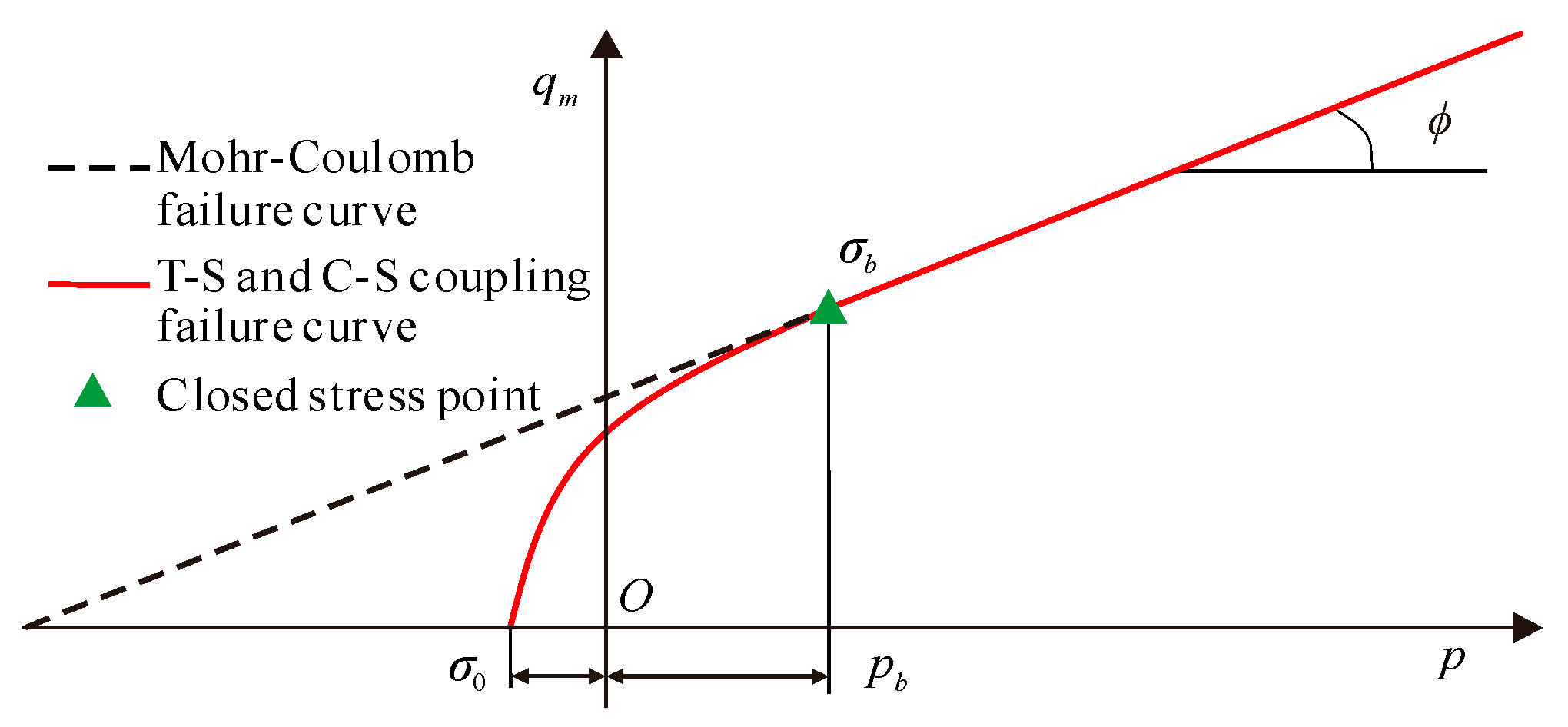
2.2. Failure Function on the Triaxial Compression Meridian Plane

Due to the influences of hydrostatic pressure (mean pressure) and T-S coupling stress, the failure curve of soil on the triaxial compression meridian is nonlinear, as shown in Figure 1. Using the reference of the concept of the closed stress point [25], the closed stress point is defined as the dividing point between the T-S coupling zone and C-S zone, which is by definition the uniaxial compression failure point. First, by establishing the failure functions in the T-S coupling and C-S stress-affected regions and then smoothly connecting the two functions at the closed stress point, we can obtain the failure function on the triaxial compression meridian plane.
Under C-S stress, the failure curve of soil on the triaxial compression meridian plane conforms to the M-C strength criterion, which can be expressed as
q m = 6 sin φ 3 sin φ p + 6 c cos φ 3 sin φ
where p = ( σ 1 + σ 2 + σ 3 ) / 3 is hydrostatic pressure; and the c and φ are the cohesion and C-S internal friction angle, respectively.
Under T-S coupling stress, the quadratic curve function q m = A m ( p + σ 0 ) 2 + B m ( p + σ 0 ) + C m is used to describe the strength in the T-S coupling zone based on the analysis of the strength test results of soils [26,27,28,29,30]. A m , B m , and C m are the coefficients which can be determined according to the geometrical relationship:
{ q m | p = σ 0 = 0 q m | p = p b = q b q m | p = p b = tan ϕ { A m = 18 sin φ ( 3 σ 0 + σ u ) ( 3 sin φ ) 9 σ u ( 3 σ 0 + σ u ) 2 B m = 6 σ u ( 3 σ 0 + σ u ) 6 sin φ ( 3 sin φ ) C m = 0
where p b = σ u / 3 and q b = σ u , which can be obtained from the definition of the uniaxial compression failure point σ b ( p b , q b ) ; σ u is the uniaxial compressive strength of soil; σ 0 = β σ t is the three-dimensional tensile strength; σ t is the uniaxial tensile strength; and β is the scale factor. σ t and σ u can be simplified as σ t = 2 c cos φ / ( 1 + sin φ ) and σ u = 2 c cos φ / ( 1 sin φ ) , respectively.
Combining the failure functions in the T-S coupling and C-S zones, we can obtain the integrated failure function of soil on the triaxial compression meridian plane:
{ q m = A m ( p + σ 0 ) 2 + B m ( p + σ 0 ) σ 0 p σ u / 3 q m = 6 sin φ 3 sin φ p + 6 c cos φ 3 sin φ p > σ u / 3  

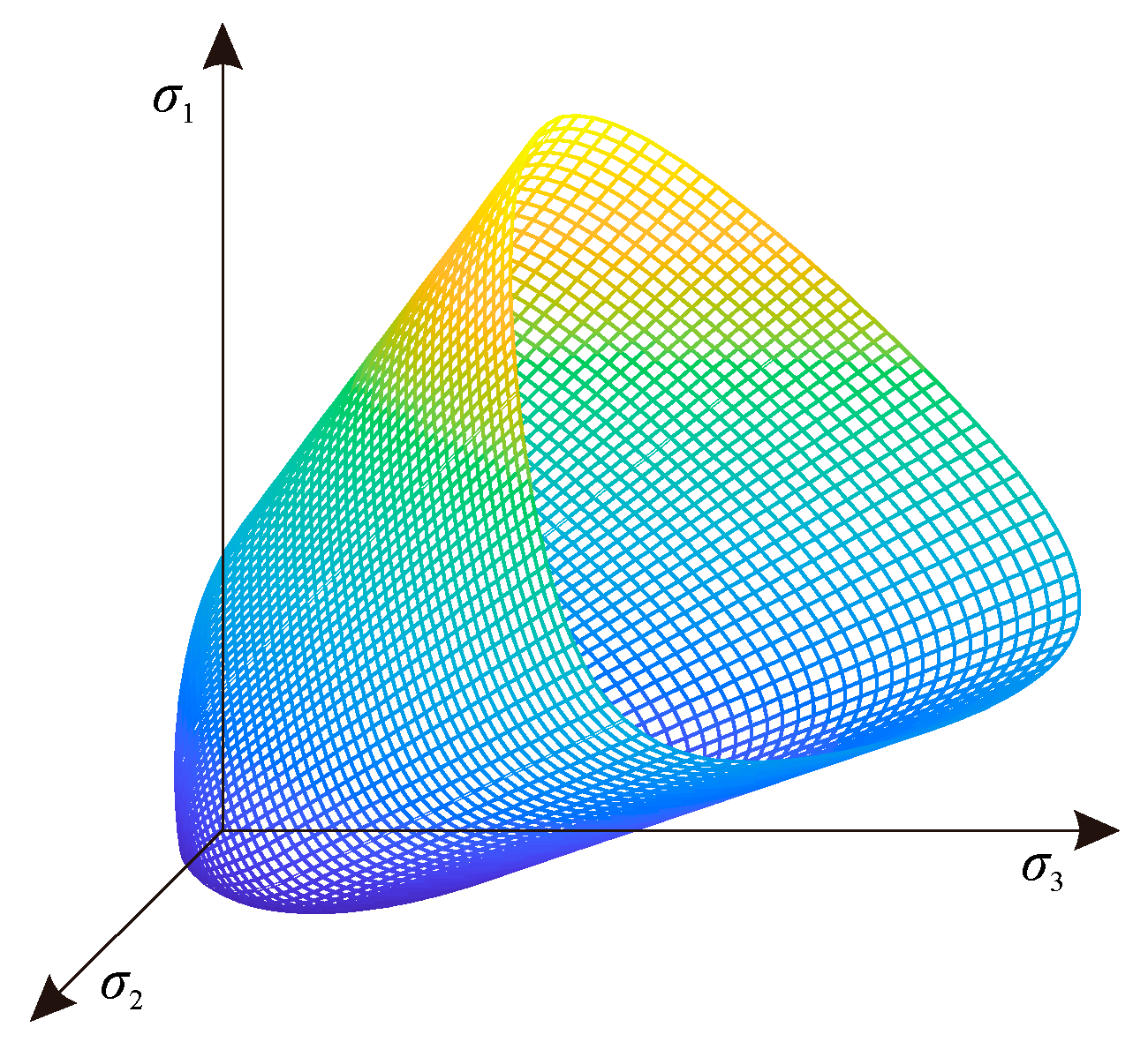
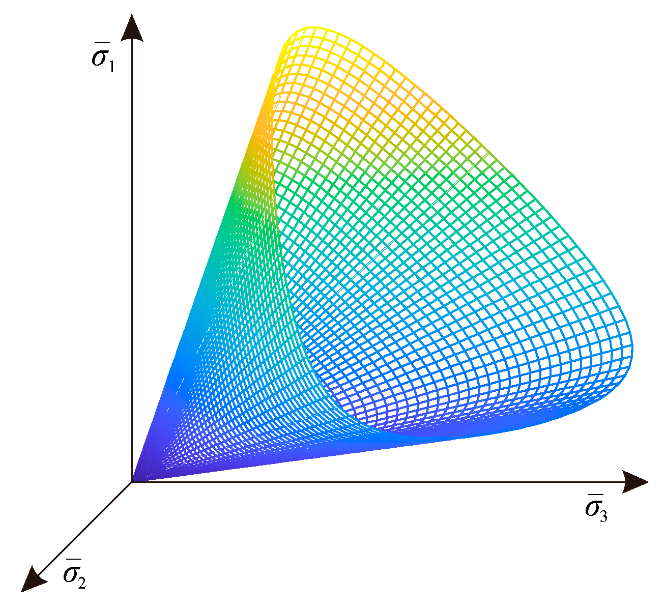
2.3. Nonlinear Strength Model in Principal Stress Space

As described in Section 2.1 and Section 2.2, the failure functions on the π plane and triaxial compression meridian plane are both nonlinear. The direct combination of the two functions would result in non-coordination between the mathematical representation and its figures [1]. Therefore, the method of linear transformation [5] is used to transform the failure function on the triaxial compression meridian plane into the linear function in a new stress space which is called transition space. As illustrated in Figure 2, the linear transformation satisfies the following relationships:
{ q ¯ m = q m q ¯ m = M f p ¯
where q ¯ m is the generalized shear stress in the transition space under triaxial compression conditions; M f is the slope of the linear failure function on the triaxial compression meridian plane in the transition space, which can be expressed as M f = 3 σ u / ( 3 σ 0 + σ u ) ; and p ¯ is the hydrostatic pressure in the transition space.
Substituting Equation (5) into Equation (4), the following general form of the stress tensor can be obtained:
{ σ ¯ i j = σ i j + [ 3 k 3 3 σ 0 + σ u ( p + σ 0 ) 2 + ( 2 k ) ( p + σ 0 ) p ] δ i j σ 0 p σ u / 3 σ ¯ i j = σ i j + [ ( k 1 ) p + k c cot φ ] δ i j p > σ u / 3
where k = 2 ( 3 σ 0 + σ u ) sin φ / [ σ u ( 3 sin φ ) ] is the model parameter; σ ¯ i j and σ i j are the stress components of transition and principal stress space, respectively; and δ i j is the Kronecker symbol.
Combining Equations (1), (5), and (6), we can obtain the nonlinear strength model:
Ι ¯ 1 2 [ 1 + 2 sin ( π 6 1 3 ( arccos Ι ¯ 1 3 54 Ι ¯ 3 Ι ¯ 1 3 ) ) ] = M f p ¯
where Ι ¯ 1 = σ ¯ 1 + σ ¯ 2 + σ ¯ 3 , Ι ¯ 3 = σ ¯ 1 σ ¯ 2 σ ¯ 3 and p ¯ = ( σ ¯ 1 + σ ¯ 2 + σ ¯ 3 ) / 3 are the first and third principal stress invariants and hydrostatic pressure in the transition space, respectively. The failure surfaces of the nonlinear strength model in the principal stress space and transition space are shown in Figure 3 and Figure 4, respectively.

3. Numerical Implementation of the Strength Model and UMAT Subroutine

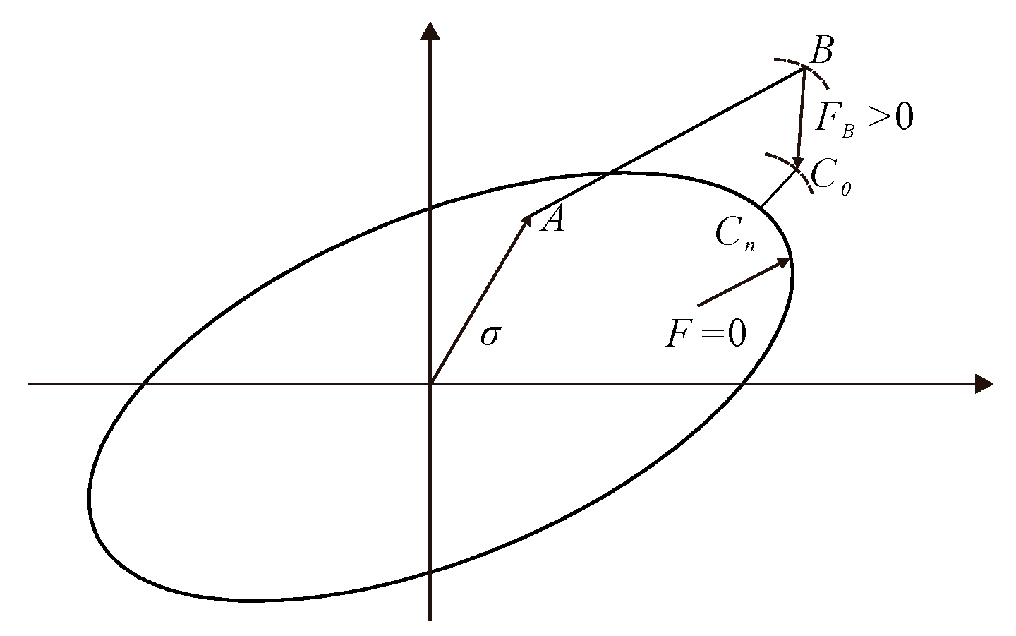
3.1. Stress Updating Algorithm

The selection of a stress updating algorithm is a key problem in the numerical realization of the elastoplastic constitutive relationship, which directly affects the efficiency and accuracy of numerical calculations. There are two kinds of stress updating algorithms: one is the explicit algorithm that is conditionally stable and strictly limited by the integral step, and the other is the implicit algorithm that is unconditionally stable. According to the user subroutines in ABAQUS, the implicit backward Euler integral algorithm is adopted [21,22,23]. When the stress exceeds the yield surface, plastic strain appears, and then the implicit backward Euler integral algorithm is used for stress adjustment to bring the stress back to the updated yield surface. The diagram of the stress updating algorithm is shown in Figure 5.
Since the tensile stress is positive in ABAQUS, the corresponding transformation of the three-dimensional nonlinear strength model has been carried out. The yield function can be expressed as follows:
F = Ι ¯ 1 2 [ 1 + 2 sin ( π 6 1 3 ( arccos Ι ¯ 1 3 54 Ι ¯ 3 Ι ¯ 1 3 ) ) ] M f p ¯
The plastic potential function G is consistent with the expression of the yield function F except that the expansion angle ψ replaces the internal friction angle φ . If ψ = φ , the flow rule is associated; otherwise, the flow rule is non-associated. When using the implicit backward Euler integral algorithm, the first-order derivative of the yield function to stress and the first-order and second-order derivatives of the plastic potential function to stress are required (refer to Appendix A).

3.2. Secondary Development of UMAT

The user material subroutine UMAT is a secondary development interface provided by ABAQUS to define the physical properties of materials. Its main task is to update the stress increments and related state variables according to the strain increments imported by the ABAQUS main program and to give the Jacobian matrix Δ σ / Δ ε of the material [31,32].
The UMAT subroutine compiled in Fortran includes the following parts: subroutine definition statements, parameter descriptions, user-defined variable descriptions, user-written programs, and return and end statements of subroutines [33,34]. The flowchart of the UMAT subroutine is shown in Figure 6; the main flow of the ABAQUS main program calling the UMAT subroutine for the solution [35,36] is as follows:
(1)
At the beginning of incremental loading step n, the ABAQUS main program transfers the stress tensor σ   t n , the total strain ε   t n , the total strain increment Δ   t n ε , and the time increment Δ t to the UMAT subroutine.
(2)
First, the elastic trial stress is calculated, and the plastic parameters are calculated with the implicit backward Euler integration algorithm. Second, the stress is pulled back to the yield surface through iterative calculation, and the consistent tangent modulus D a lg , the Jacobian matrix, is calculated. Finally, the stress increment Δ σ = D   t n a lg Δ   t n ε can be calculated, and the stress is updated to σ   t n + Δ t = σ   t n + Δ σ .
(3)
At time t n + 1 , the ABAQUS main program uses the Newton–Raphson iterative method to perform the iterative calculations. If the calculation result converges, the next incremental step is performed with n = n + 1 ; if not, the time increment Δ t of the incremental step is reduced until the calculation result converges.

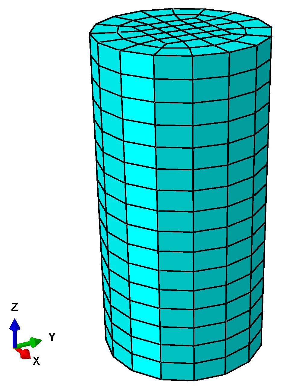
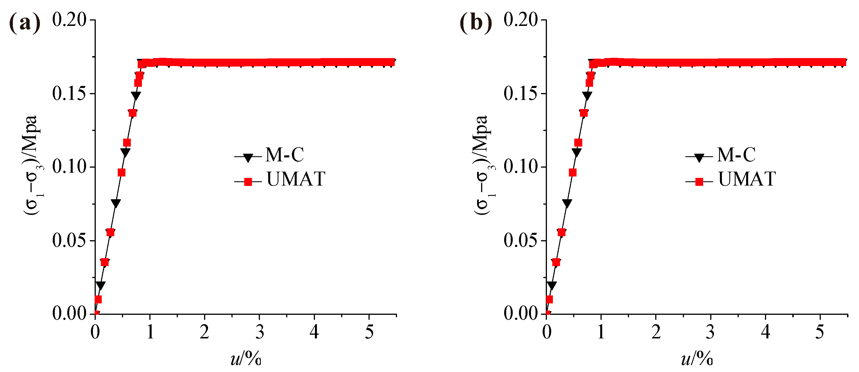
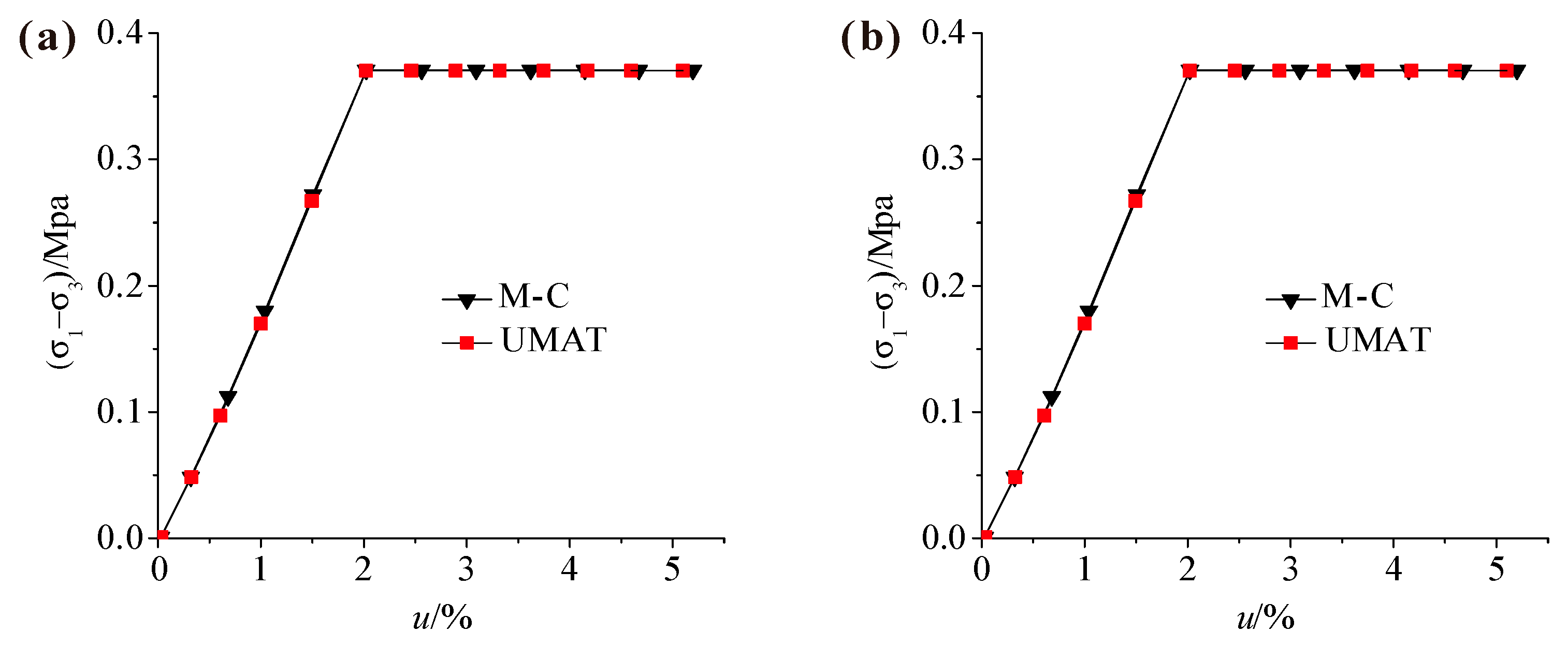
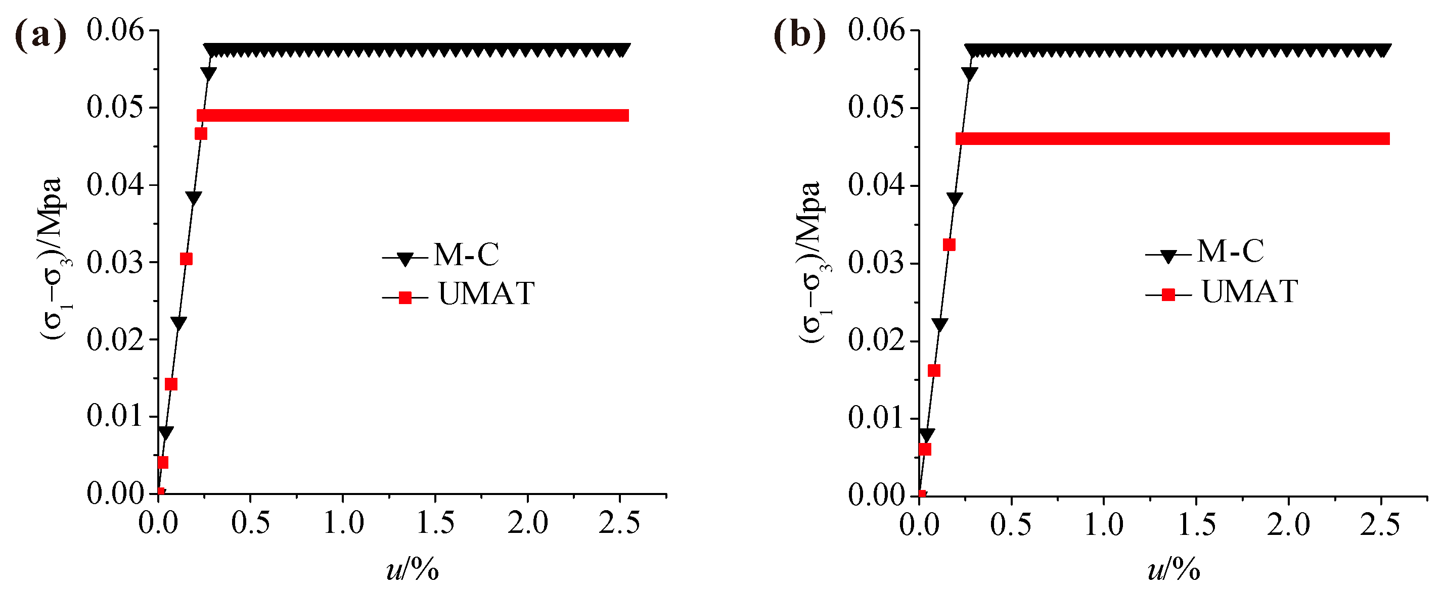
3.3. UMAT Subroutine Verification

After compiling and debugging the UMAT subroutine based on the three-dimensional nonlinear strength model of soil, a finite element analysis of conventional soil mechanics tests under triaxial compression and uniaxial tension is conducted. Through comparative analysis of the calculation results of the UMAT subroutine and M-C model embedded in ABAQUS, the calculation ability and the accuracy and efficiency of the developed UMAT subroutine are verified.

3.3.1. Triaxial Compression Test

The element type of the triaxial specimen with a diameter of 50 mm and height of 100 mm is a fully integrated C3D8 solid element; the analysis model is shown in Figure 7. Applying a displacement load of 5 mm along the negative direction of the Z-axis with the displacements restrained in all directions of the Z = 0 surface, calculations under confining pressures of 0 kPa and 100 kPa are carried out. The material parameters are shown in Table 1.
The test results under uniaxial and triaxial compression are shown in Figure 8 and Figure 9, respectively, with the scale factor β assuming different values. According to the comparison of the test results, the calculation results of the UMAT subroutine are the same as those of the M-C model, and the yield stresses of the two are equal. This is mainly because under uniaxial and triaxial compression, the yield surface is in the C-S zone. Only the shear deformation caused by compression is produced, which results in the coincidence of the yield surfaces of the two strength models. Moreover, the scale factor β only contributes to the strength of the T-S coupling zone, not the C-S zone; therefore, the stress–strain relationships are consistent when β is 1 and 0.9.

3.3.2. Uniaxial Tensile Test

The calculation model and material parameters of the uniaxial tensile tests are consistent with those of the triaxial compression tests in the previous section. A displacement load of 2 mm is applied along the positive direction of the Z-axis, with the displacements restrained in all directions of the Z = 0 surface.
The calculation results under uniaxial tension are shown in Figure 10, assuming different values for β . From the comparison of stress–strain relationships, it can be found that the soil element of the UMAT subroutine enters the plastic state earlier, and the yield stress is less than that of the M-C model; with the decrease in β , the UMAT yield stress decreases gradually. This is because the yield surface is in the T-S coupling zone under uniaxial tension, and the uniaxial tensile strength of the three-dimensional nonlinear strength model slightly decreases with the decrease in β . Still, the conventional M-C model significantly overestimates the tensile properties of soil. Therefore, based on the tenso-shear performance of actual soil, we can adjust the T-S coupling zone through β . The calculation results of the UMAT subroutine are more practical under T-S coupling stress.

4. Numerical Examples of Saturated Slope

In the analysis of slope stability, it is necessary to clarify the failure mechanism of slopes. The instability failure of the slope is the result of the coaction of T-S coupling failure and C-S failure; therefore, the slope body’s T-S coupling failure and C-S failure should be considered simultaneously in slope stability analysis. Based on the three-dimensional nonlinear strength model, the reduction of the C-S strength parameters [37] is as follows:
c m = c F r , φ m = arctan ( tan φ F r )
where F r is the safety factor; and c m and φ m are the mobilized cohesion and internal friction angle of the soil, respectively.
Since the parameters σ 0 and σ u are simplified in the numerical implementation of the model, the yield function F is directly related to the C-S strength parameters c and φ ( tan φ ) . Therefore, the changes in σ 0 and σ u can be described by Equation (9) during strength reduction. The yield and plastic potential functions in the T-S coupling and C-S zones are updated continuously, thereby avoiding the incompatibility problem.

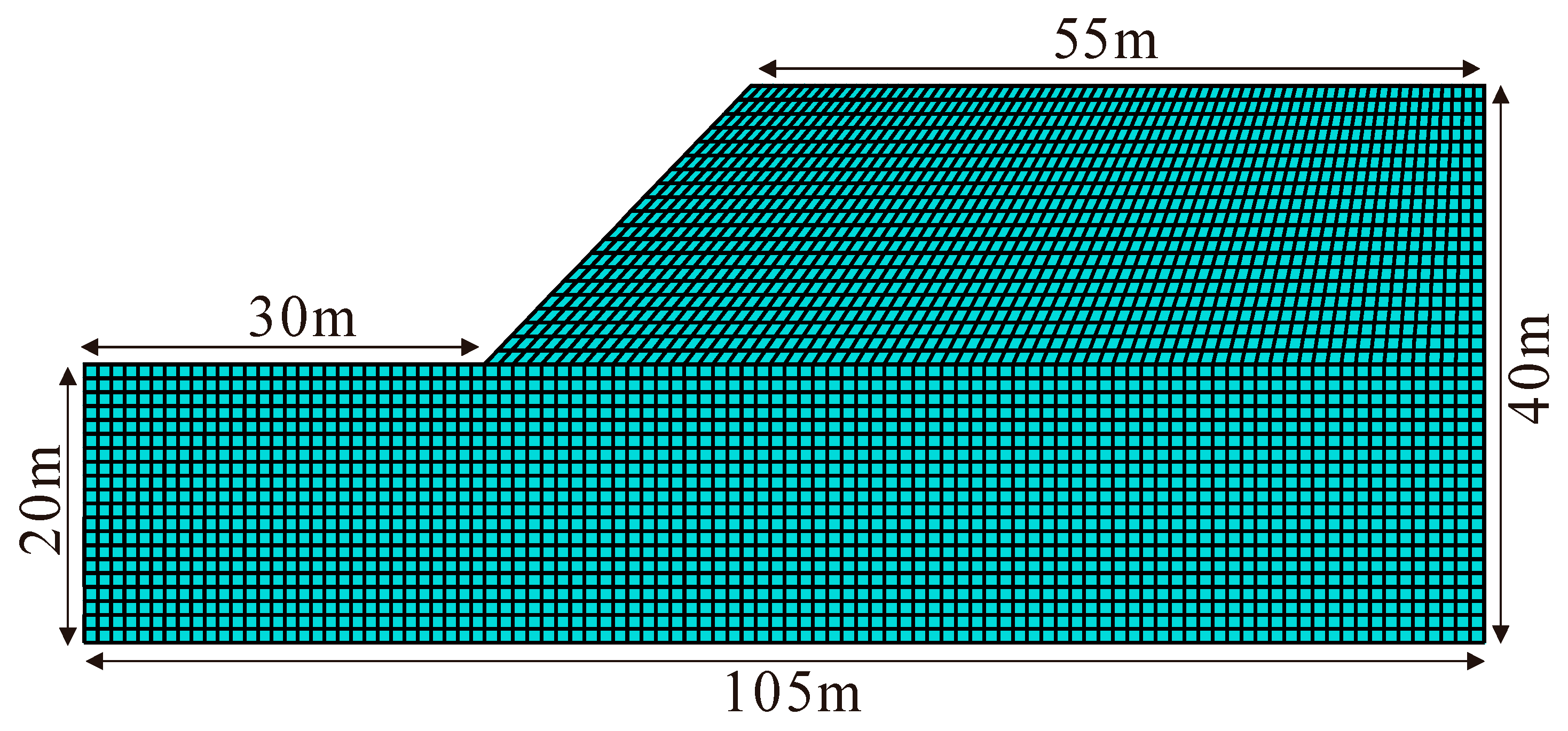
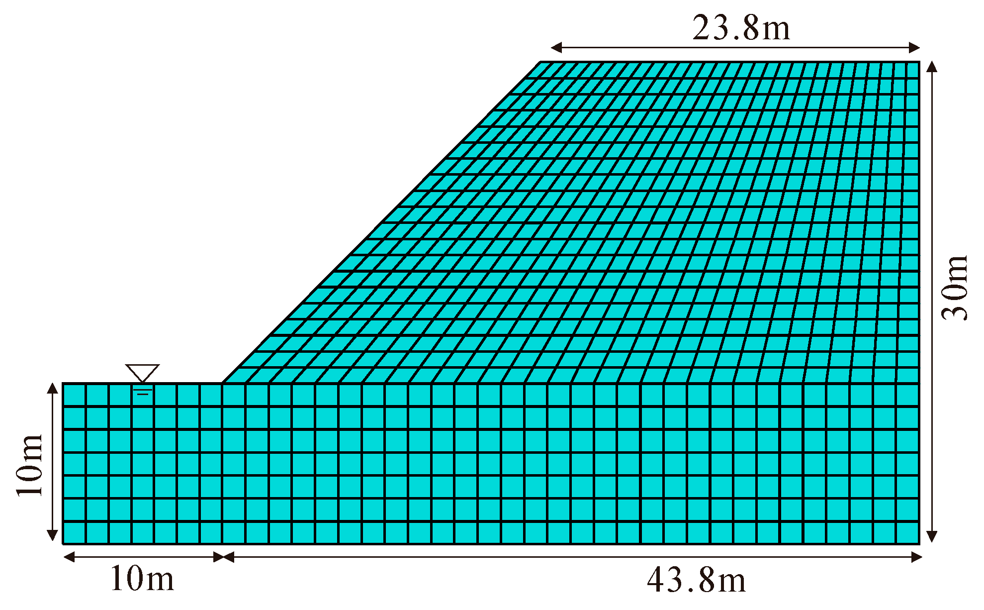
4.1. Analysis Model of Slope

A classic model [38] of saturated slopes is selected to analyze the mechanism of slope deformation and failure; the analysis model is shown in Figure 11. The boundary conditions are horizontal constraints on the left and right sides, horizontal and vertical constraints at the bottom, and free boundaries on the slope surfaces. The yield criteria for the soil as an ideal elastoplastic material are the M-C yield criterion and the three-dimensional nonlinear yield criterion. The material parameters of the soil are shown in Table 2.

4.2. Slope Analysis Based on M-C Strength Model

First, according to the M-C yield criterion, the calculation of the associated flow ( ψ = φ ) is carried out. The equivalent plastic strain (shear strain) nephogram and maximum principal stress nephogram of the unstable slope are shown in Figure 12 and Figure 13, respectively. The slope safety factor is 1.24 when taking the run-through of the plastic zone as the instability criterion. According to the calculation results, under the influence of self-weight stress, the upper slope is in the tensile stress area within a certain depth from the top surface; when the slope is unstable, the slope in the tensile stress area is subjected to T-S coupling stress and results in T-S coupling failure. However, the equivalent plastic zone of the slope obtained by the M-C yield criterion cannot describe the upper slope’s T-S coupling failure, and the slope’s critical slip surface is a C-S slip surface that develops from the slope toe upward to the top surface of the slope.

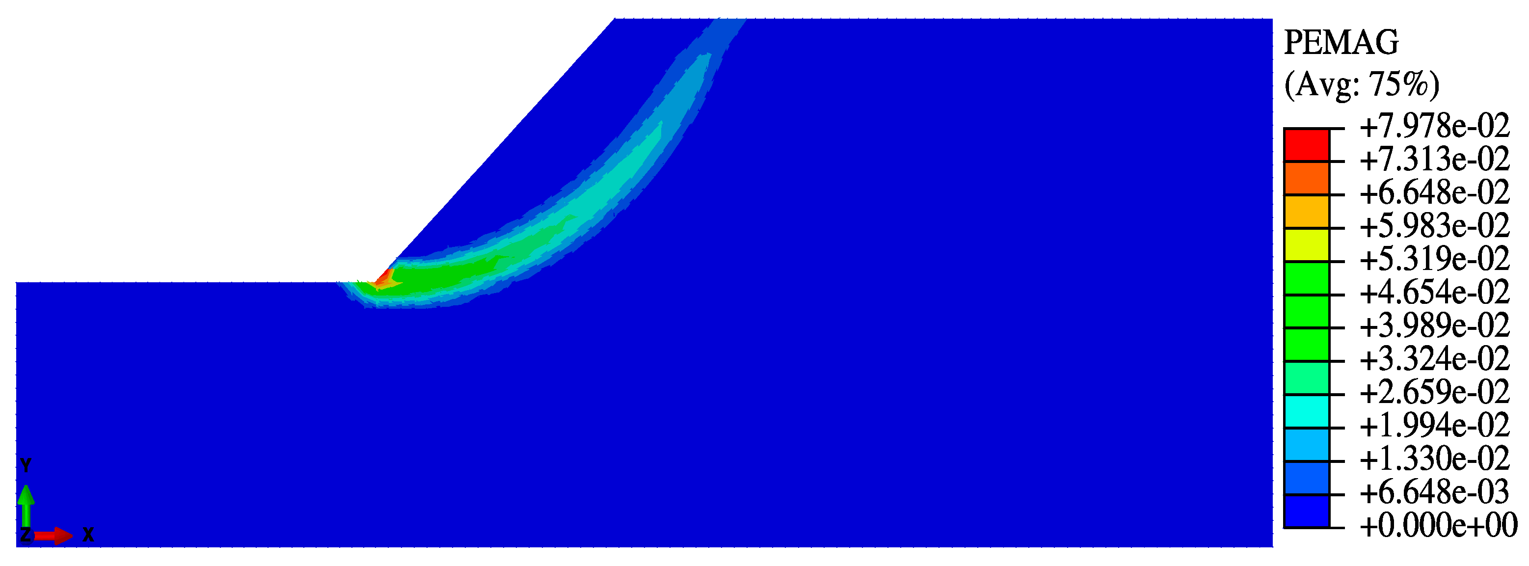
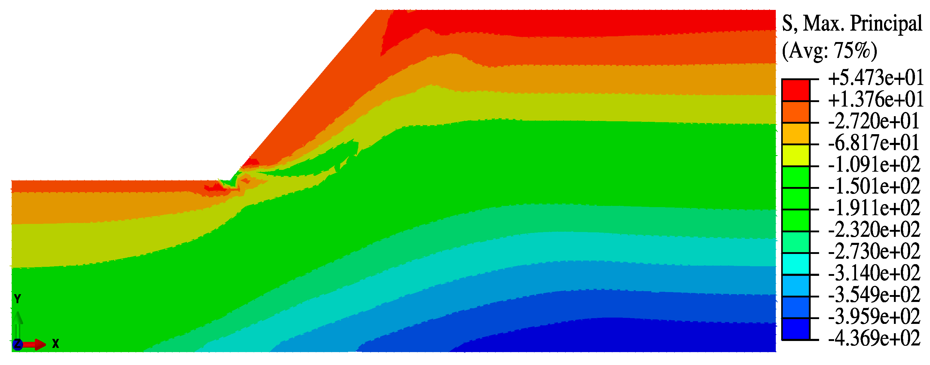
4.3. Slope Analysis Based on Three-Dimensional Nonlinear Strength Model

According to the nonlinear yield criterion, the calculation of associated flow is carried out, taking β = 1 and β = 0.9 . Figure 14 shows the development of the equivalent plastic zone of the progressively unstable slope. To clearly illustrate and compare the instability processes under different yield criteria, three calculation steps are selected during slope instability from the near instability to the final instability in Figure 14, and the slope graphs are intercepted for the convenience of comparison. Figure 14a,b shows that when the slope approaches instability, a T-S coupling plastic zone generated from the top surface of the slope gradually develops downward and finally connects with the equivalent plastic zone that develops upward from the slope toe, resulting in the instability of the slope. However, Figure 14c shows that the equivalent plastic zone obtained by the M-C yield criterion develops upward from the slope toe and reaches the top surface to produce a plastic penetration zone. Therefore, the three-dimensional nonlinear yield criterion can better describe the T-S coupling failure of the upper slope. Taking the run-through of the plastic zone as the instability criterion, the safety factors of the slope are 1.23 and 1.226 when β = 1 and β = 0.9 , respectively.
The maximum principal stress nephograms and critical slip surfaces of unstable slopes with T-S coupling strength are shown in Figure 15 and Figure 16, respectively. During the development of the slip surface, plastic deformation first appears in the C-S zone and results in the C-S slip surface developing upward from the slope toe; when the slip surface develops to the T-S coupling zone, the T-S coupling failure surface develops upward from the interface and downward from the top surface of the slope, finally forming a continuous failure surface. The critical slip surface is a composite slip surface composed of a C-S slip surface and a T-S coupling failure surface.
Comparing the calculation results of the three-dimensional nonlinear yield criterion and M-C yield criterion, the following can be determined: (1) The range of the tensile stress zone in the unstable slope based on the two yield criteria is the same. Still, the maximum tensile stress value in the tensile stress zone of the former decreases with the decrease in β (51.66 kPa for β = 1 and 49.77 kPa for β = 0.9 ), and is less than that of the latter (54.73 kPa). (2) The former can give a reasonable T-S coupling plastic zone and T-S coupling failure surface and clearly describe their progressive developments. (3) The safety factor obtained by the former is less than that obtained by the latter and gradually decreases with decreasing β (M-C, F r = 1.24 ; β = 1 , F r = 1.23 ; β = 0.9 , F r = 1.226 ).
This is because the M-C yield criterion does not consider T-S coupling stress, so it overestimates the T-S coupling strength of soil and obtains a larger safety factor that is dangerous in practice. The three-dimensional nonlinear yield criterion can reasonably describe the strength characteristics of soil under T-S coupling stress and adjust the T-S coupling zone through β , reflecting the actual soil’s T-S performance. Accordingly, the three-dimensional nonlinear yield criterion can give a reasonable T-S coupling failure area, and the obtained safety factor is relatively small.

5. Numerical Examples of Unsaturated Slope

Based on the three-dimensional nonlinear strength model, the stability of unsaturated slopes under the conditions of no rainfall and rainfall infiltration are analyzed by using the strength reduction finite element method under fluid–solid coupling [39,40]. Compared with the calculation results of the M-C strength model, the applicability and accuracy of the three-dimensional nonlinear strength model in the stability analysis of unsaturated soil slopes are discussed.
In the finite element calculation, the additional strength under the combined action of matrix suction and saturation can be simplified as follows [41,42]:
( u a u w ) S e tan φ
where S e is the effective degree of saturation.
Thus, the C-S strength formula of unsaturated soils has the following expression:
τ f c = c + ( σ u a ) tan φ + ( u a u w ) S e tan φ
The soil–water characteristic curve is described by the Van Genuehten model [43], and the relationship between effective saturation and matrix suction is as follows:
S e = { 1 1 + [ α ( u a u w ) ] n } 1 1 / n
where α and n are the fitting parameters related to the air entry value and pore distribution, respectively. Since the slope is connected to the atmosphere, the pore pressure can be taken as zero in slope analysis; thus, the matrix suction can be expressed by negative pore water pressure.
The permeability coefficient of unsaturated soil, which cannot generally be regarded as a constant like saturated soil, is associated with matrix suction (or volumetric water content). Based on the Mualem model [44] and Van Genuehten soil–water characteristic curve [43], the permeability coefficient of unsaturated soil can be expressed as follows:
k w = k r ( S e ) k s = S e 1 / 2 [ 1 ( 1 S e n / ( n 1 ) ) 1 1 / n ] 2 k s
where k r is the relative permeability coefficient and k s is the saturated permeability coeficient.

5.1. Analysis Model of Slope

A soil slope 20 m in height and 45° in slope gradient, with the groundwater level at the toe, is selected to analyze the stability of unsaturated slopes. The soil in the slope composed of homogeneous silt, with its material parameters in Table 3, is regarded as an ideal elastoplastic material. The calculation model of the slope is shown in Figure 17. The associated flow law is adopted in the calculation. The boundary conditions are given as follows: (1) Displacement boundary conditions: the left and right sides are horizontally constrained; bottom side is horizontally and vertically constrained, and the other sides (slope surfaces) are free boundaries. (2) Pore pressure boundary conditions: the left and right sides below the slope toe are set as the static water pore pressure boundary that increases linearly with depth. (3) Seepage boundary conditions: the left, right, and bottom sides are waterproof boundaries; the slope surfaces are all permeable boundaries. (4) Rainfall boundary conditions: the slope surfaces are all flux boundaries when rainfall occurs.

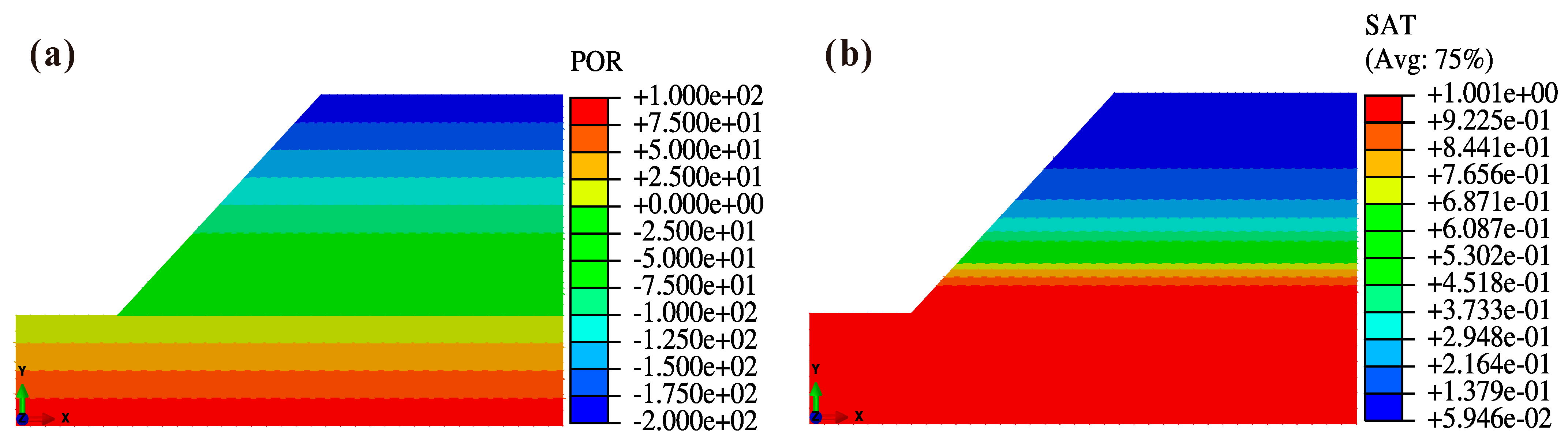
5.2. Unsaturated Slope without Rainfall

Before the stability analysis of the unsaturated slope, the effect of the static water level is analyzed first, and a series of initial conditions (such as pore pressure, effective saturation, pore ratio, and stress distribution of the slope) are obtained, which are the initial states of subsequent analysis (the initialization of the stress states involving geological history and loading history [45] is not involved in this paper). The distributions of pore pressure and effective saturation at the initial state are shown in Figure 18.
The development of the equivalent plastic zone of the progressively unstable slope is shown in Figure 19; the slope graphs are intercepted for the convenience of comparison. Figure 19 shows that the equivalent plastic zone obtained by the M-C yield criterion develops upward from the slope toe and reaches the top surface of the slope to produce a plastic penetration zone. However, based on the nonlinear yield criterion ( β = 0.9 ), when the slope approaches instability, a T-S coupling plastic zone generated from the top surface of the slope gradually develops downward and finally connects with the equivalent plastic zone that extends upward from the slope toe. Taking the run-through of the plastic zone as the instability criterion, the safety factors of the slope based on the two yield criteria are 1.516 and 1.504.
The maximum principal stress nephograms and critical slip surfaces of unstable slopes are shown in Figure 20 and Figure 21, respectively. Based on the M-C yield criterion, the critical slip surface is a C-S slip surface that develops from the slope toe upward to the top surface of the slope. However, based on the nonlinear yield criterion, the critical slip surface is a composite slip surface composed of a C-S slip surface and a T-S coupling failure surface. Figure 20 shows that the range of the tensile stress zone and the maximum value of tensile stress based on the two yield criteria are relatively small. This is because the suction in slope increases with height; thus, the additional strength due to the suction and the degree of saturation also increase with height. As a result, the T-S coupling strength of slope soil increases with height. During the slope instability, the higher the height of soil is, the later its time of entering the tensile stress zone; therefore, the tensile stress value and the range of the tensile stress zone are small when the slope becomes unstable.
Comparing the calculation results of the three-dimensional nonlinear yield criterion and M-C yield criterion, conclusions similar to the numerical examples of saturated slopes can be found: (1) The safety factor obtained by the former (1.504) is less than that of the latter (1.516). (2) The former can give a reasonable T-S coupling plastic zone and T-S coupling failure surface and clearly describe their progressive developments. (3) The range of the tensile stress zone in the unstable slope based on the two yield criteria is the same, but the maximum tensile stress value in the tensile stress zone of the former (32.20 kPa) is less than that of the latter (41.48 kPa).

5.3. Unsaturated Slope with Rainfall Infiltration

Due to the complicated rainfall infiltration process, which is closely correlated with factors such as rainfall intensity and soil properties, the rainfall process is simplified. In this example, the rainfall boundary function is expressed in terms of rainfall intensity (that is, flow flux q (m/s)); moreover, the runoff of slope is activated. The rainfall intensity is taken as 0.01 m/h (2.78 × 10⁻⁶ m/s); rainfall with a 72 h duration will affect the top and surface of the slope. Figure 18 illustrates the distributions of pore water pressure and effective saturation after 72 h of rainfall. Figure 22 shows that a transient saturation zone occurs on the surface layer of the slope, and that the effective saturation in the shallow layer of the slope (especially the slope body above the toe) increases with the significant increase in pore water pressure and the reduction or disappearance of matrix suction. However, the increase in effective saturation of soil inside the slope body is slight, and the pore water pressure exhibits little change.
The safety factors of the slope are 1.381 and 1.368 based on the nonlinear yield criterion ( β = 0.9 ) and M-C yield criterion, respectively; the equivalent plastic zones and critical slip surfaces of the unstable slope are shown in Figure 23. Comparing the calculation results of the two yield criteria, conclusions similar to the previous section can be found: the three-dimensional nonlinear yield criterion can clearly describe the progressive developments of the T-S coupling plastic zone and T-S coupling failure surface; the critical slip surface is a composite slip surface composed of a C-S slip surface and a T-S coupling failure surface; and the safety factor obtained is relatively small, which is safe in practice.

6. Conclusions

Taking the intermediate principal stress effect and T-S coupling strength mechanism in soil into account, a three-dimensional nonlinear strength model of soil is established. Based on this model, a UMAT subroutine in which the constitutive relationship is programmed using an implicit backward Euler integration algorithm is secondarily developed with the ABAQUS platform. Through triaxial compression and uniaxial tension numerical tests, the accuracy was determined. The effectiveness of the program algorithm is verified. Subsequently, the UMAT subroutine is applied to the analysis of slope stability, and the following works are carried out:
(1)
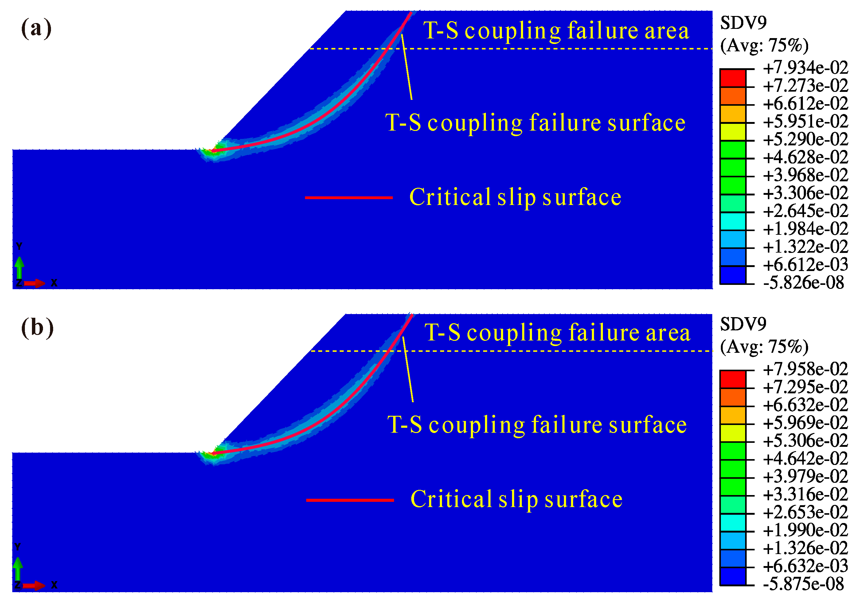
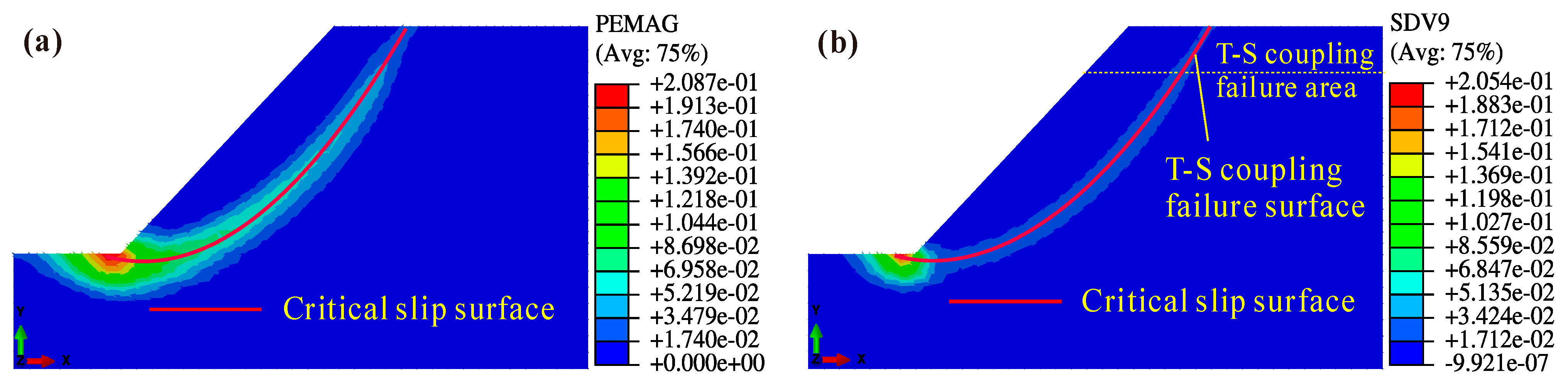
For saturated slopes, a comparative analysis of the calculation results between the three-dimensional nonlinear strength model and the MC strength model, using the strength reduction finite element method, is conducted. The three-dimensional nonlinear strength model proposed in this paper can better describe the gradual development processes of the T-S coupling plastic zone and T-S coupling failure surface. The critical slip surface is a composite slip surface composed of a C-S slip surface and T-S coupling failure surface, and the obtained safety factor is small and inclined to be safe.
(2)
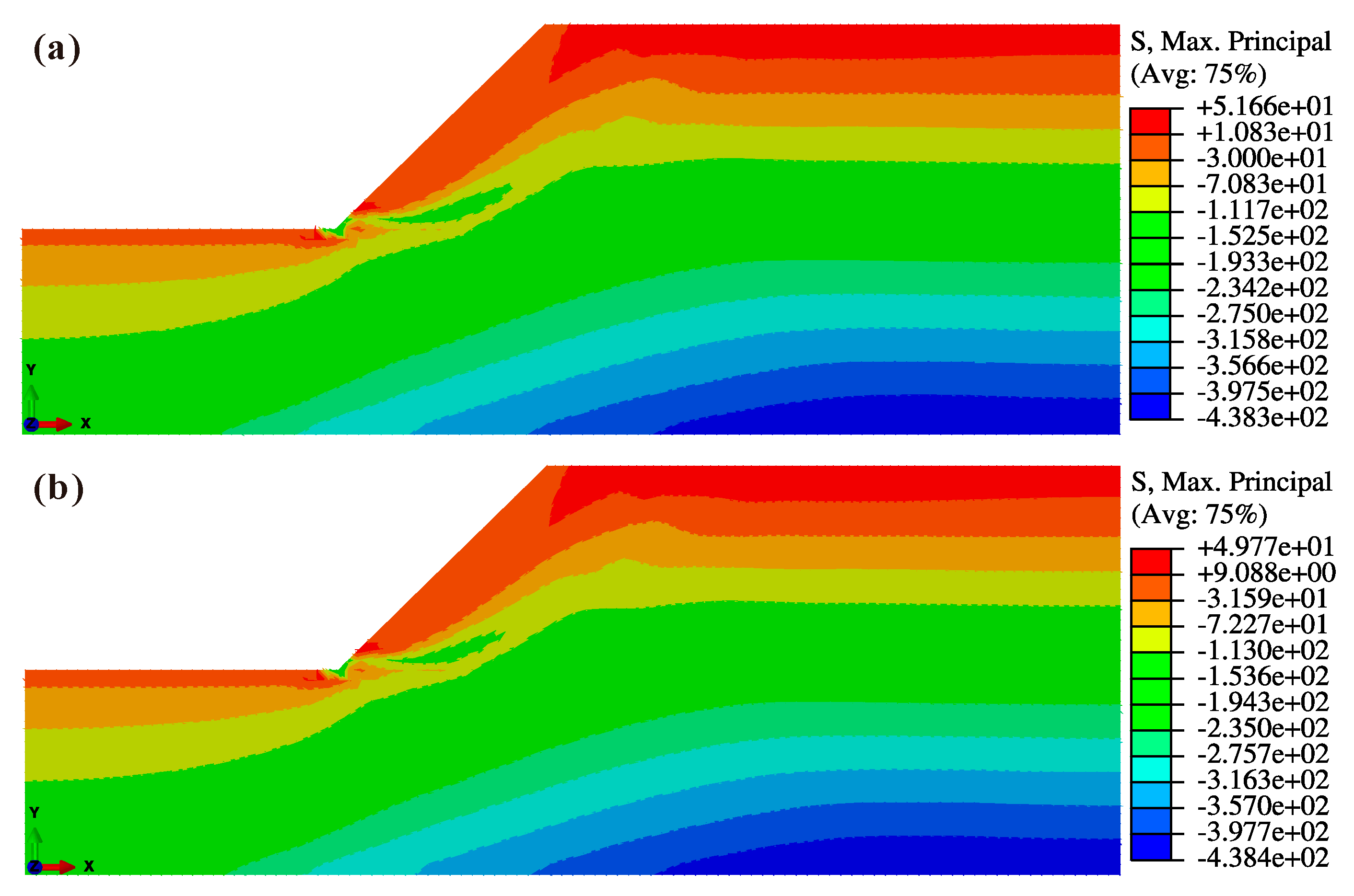
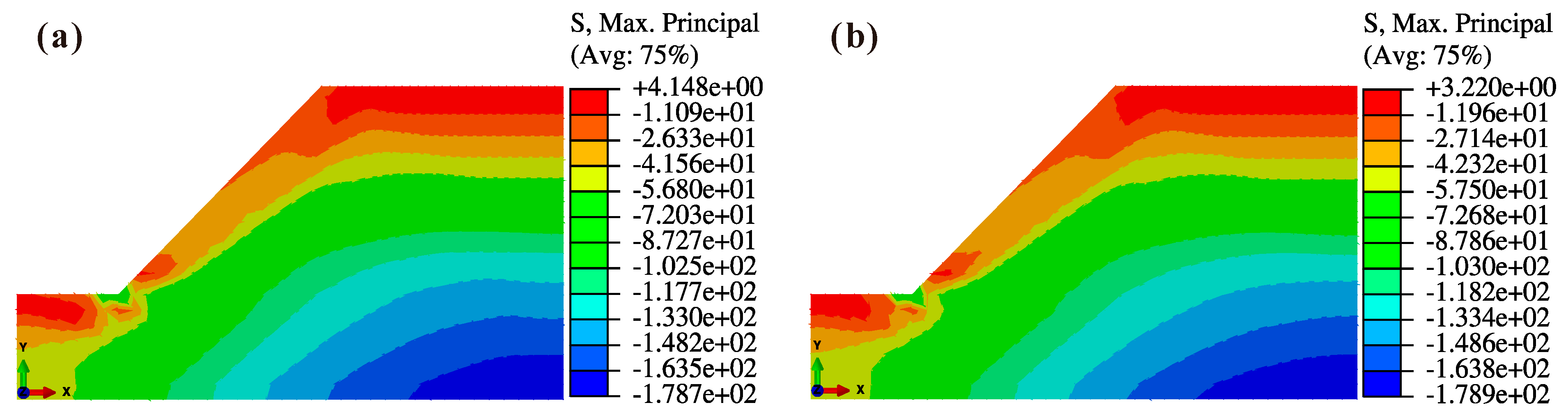
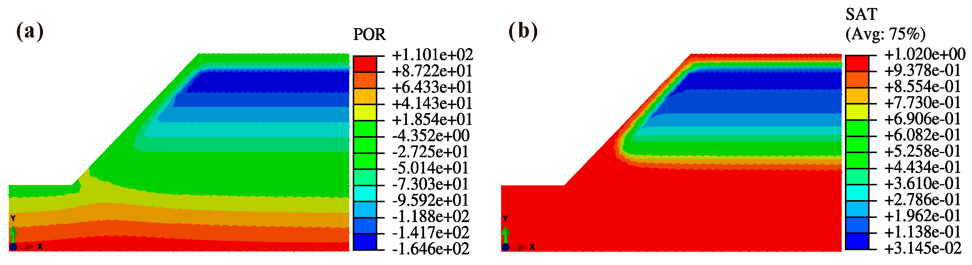
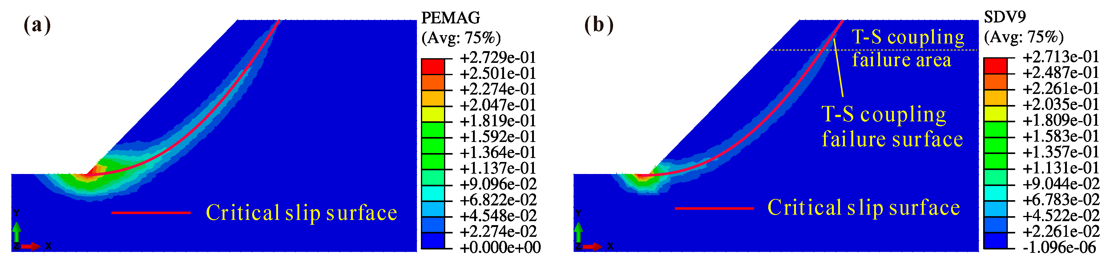
For unsaturated soil slopes, the stabilities of slopes under the conditions of no rainfall and rainfall infiltration are analyzed by using the strength reduction finite element method under fluid–solid coupling. Compared with the calculation results of the M-C strength model, the three-dimensional nonlinear strength model shows apparent advantages, which are the same as the conclusions from the analysis of saturated slopes.
The above research shows that the proposed model can better explain slope deformation failure mechanisms, describe the progressive developments of the equivalent plastic zones and critical slip surfaces, and provide more accurate slope stability evaluation; thus, it has particular practical value. The three-dimensional nonlinear strength model will be used for engineering cases of slopes in future research. Research on the stability of clay slopes for specific geographical environments and geological conditions (such as the mountain areas of southwest China) will also be conducted.

Author Contributions

Conceptualization, X.K. and C.Z.; methodology, software, investigation, and writing—original draft preparation, X.K.; supervision, G.C.; writing—review and editing, X.K., G.C., Y.C. and C.Z.; funding acquisition, G.C. and Y.C. All authors have read and agreed to the published version of the manuscript.

Funding

This research was funded by the National Natural Science Foundation of China, grant number U2034204, 52078031; the Beijing Natural Science Foundation, grant number 8202038; the Fundamental Research Funds for the Central Universities, grant number 2020JBM048, 2020CZ002; the China State Construction Engineering Corporation, grant number CSCEC-2019-Z-09; and the National Key R&D Program of China, grant number 2018YFC0809400.

Institutional Review Board Statement

Not applicable.

Informed Consent Statement

Not applicable.

Data Availability Statement

Some or all data, models, or code that support the findings of this study are available from the corresponding author upon reasonable request.

Conflicts of Interest

The authors declare no conflict of interest.

Appendix A

Define a as the first-order derivative of the yield function to stress; its expression is
a = F σ i j = F σ ¯ i j σ ¯ i j σ i j = ( F I ¯ 1 I ¯ 1 σ ¯ i j + F I ¯ 3 I ¯ 3 σ ¯ i j ) σ ¯ i j σ i j
where
I ¯ 1 σ ¯ i j = δ i j = [ 1 , 1 , 1 , 0 , 0 , 0 ] T , I ¯ 3 σ ¯ i j = I ¯ 2 δ i j I ¯ 1 σ ¯ j i + σ ¯ j k σ ¯ k i
F I ¯ 1 = F I ¯ 1 + cos ( π 6 1 3 ( arccos Ι ¯ 1 3 54 Ι ¯ 3 Ι ¯ 1 3 ) ) 9 Ι ¯ 3 3 Ι ¯ 3 ( Ι ¯ 1 3 27 Ι ¯ 3 )
F I ¯ 3 = cos ( π 6 1 3 ( arccos Ι ¯ 1 3 54 Ι ¯ 3 Ι ¯ 1 3 ) ) 3 Ι ¯ 1 3 Ι ¯ 3 ( Ι ¯ 1 3 27 Ι ¯ 3 )
{ σ ¯ i j σ i j = 6 ( 1 k ) 3 σ 0 + σ u ( p σ 0 ) + ( 2 k ) σ u / 3 p σ 0 σ ¯ i j σ i j = k p < σ u / 3
Define b as the first-order derivative of the plastic potential function to stress; its expression is similar to a :
b = G σ i j = G σ ¯ i j σ ¯ i j σ i j = ( G I ¯ 1 I ¯ 1 σ ¯ i j + G I ¯ 3 I ¯ 3 σ ¯ i j ) σ ¯ i j σ i j
where
G I ¯ 1 = G I ¯ 1 + cos ( π 6 1 3 arccos C 1 ) C 2 , G I ¯ 3 = cos ( π 6 1 3 arccos C 1 ) C 3
C 1 = Ι ¯ 1 3 54 Ι ¯ 3 Ι ¯ 1 3 , C 2 = 9 Ι ¯ 3 3 Ι ¯ 3 ( Ι ¯ 1 3 27 Ι ¯ 3 ) , C 3 = 3 Ι ¯ 1 3 Ι ¯ 3 ( Ι ¯ 1 3 27 Ι ¯ 3 )
{ σ ¯ i j σ i j = 6 6 k ( ψ ) 3 σ 0 + σ u ( p σ 0 ) + 2 k ( ϕ ) σ u / 3 p σ 0 σ ¯ i j σ i j = k ( ψ ) p < σ u / 3
k ( ψ ) = 2 ( 3 σ 0 + σ u ) sin ψ σ u ( 3 sin ψ )
The second-order derivative of the plastic potential function to stress has the following expression:
2 G σ i j 2 = b σ i j = 2 G I ¯ 1 σ i j I ¯ 1 σ i j + 2 G I ¯ 3 σ i j I ¯ 3 σ i j + 2 I ¯ 3 σ ¯ i j σ i j G I ¯ 3 σ ¯ i j σ i j + G σ ¯ i j 2 σ ¯ i j σ i j 2
where
2 G I ¯ 1 σ i j = b I ¯ 1 G I ¯ 1 2 σ ¯ i j σ i j δ i j sin ( π 6 1 3 arccos C 1 ) 3 1 C 1 2 C 1 σ i j C 2 + cos ( π 6 1 3 arccos C 1 ) C 2 σ i j
2 G I ¯ 3 σ i j = sin ( π 6 1 3 arccos C 1 ) 3 1 C 1 2 C 1 σ i j C 3 cos ( π 6 1 3 arccos C 1 ) C 3 σ i j
{ C 1 σ i j = 54 Ι ¯ 1 4 ( 3 Ι ¯ 3 I ¯ 1 σ ¯ i j Ι ¯ 1 I ¯ 3 σ ¯ i j ) σ ¯ i j σ i j C 2 σ i j = C 2 3 Ι ¯ 1 2 54 Ι ¯ 3 2 ( 3 Ι ¯ 3 I ¯ 1 σ ¯ i j Ι ¯ 1 I ¯ 3 σ ¯ i j ) σ ¯ i j σ i j C 3 σ i j = C 3 3 6 Ι ¯ 1 3 [ Ι ¯ 3 ( Ι ¯ 1 3 + 54 Ι ¯ 3 ) I ¯ 1 σ ¯ i j + Ι ¯ 1 ( Ι ¯ 1 3 54 Ι ¯ 3 ) I ¯ 3 σ ¯ i j ] σ ¯ i j σ i j
{ 2 σ ¯ i j σ i j 2 = 2 2 k ( ψ ) 3 σ 0 + σ u δ i j σ u / 3 p σ 0 2 σ ¯ i j σ i j 2 = 0 p < σ u / 3
2 I ¯ 3 σ ¯ i j σ i j = 2 I ¯ 1 σ ¯ i j σ i j

References

  1. Yao, Y.P.; Lu, D.C.; Zhou, A.N.; Bo, Z. Generalized non-linear strength theory and transformed stress space. Sci. China Ser. E Technol. Sci. 2004, 47, 691–709. [Google Scholar] [CrossRef]
  2. Matsuoka, H.; Hoshikawa, T.; Ueno, K. A general failure criterion and stress-strain relation for granular materials to metals. Soils Found. 1990, 30, 119–127. [Google Scholar] [CrossRef] [Green Version]
  3. Lade, P.V.; Duncan, J.M. Elastoplastic stress-strain theory for cohesionless soil. J. Geotech. Eng. Div. 1975, 101, 1037–1053. [Google Scholar] [CrossRef]
  4. Lade, P.V. Estimating parameters from a single test for the three-dimensional failure criterion for frictional materials. J. Geotech. Geoenviron. Eng. 2014, 140, 4014038. [Google Scholar] [CrossRef]
  5. Yao, Y.P.; Zhou, A.N.; Lu, D.C. Extended transformed stress space for geomaterials and its application. J. Eng. Mech. 2007, 133, 1115–1123. [Google Scholar] [CrossRef]
  6. Choi, K.Y.; Cheung, R.W.M. Landslide disaster prevention and mitigation through works in Hong Kong. J. Rock Mech. Geotech. Eng. 2013, 5, 354–365. [Google Scholar] [CrossRef] [Green Version]
  7. Cai, G.Q.; Shi, P.X.; Kong, X.A.; Zhao, C.G.; Likos, W.J. Experimental study on tensile strength of unsaturated fine sands. Acta Geotech. 2020, 15, 1057–1065. [Google Scholar] [CrossRef]
  8. Zienkiewicz, O.C.; Humpheson, C.; Lewis, R.W. Associated and non-associated visco-plasticity and plasticity in soil mechanics. Geotechnique 1975, 25, 671–689. [Google Scholar] [CrossRef]
  9. Ugai, K. A method of calculation of total safety factor of slope by elasto-plastic FEM. Soils Found. 1989, 29, 190–195. [Google Scholar] [CrossRef] [Green Version]
  10. Ugai, K.; Leshchinsky, D.O.V. Three-dimensional limit equilibrium and finite element analyses: A comparison of results. Soils Found. 1995, 35, 1–7. [Google Scholar] [CrossRef]
  11. Griffiths, D.V.; Lane, P.A. Slope stability analysis by finite elements. Geotechnique 1999, 49, 387–403. [Google Scholar] [CrossRef]
  12. Lane, P.A.; Griffiths, D.V. Assessment of stability of slopes under drawdown conditions. J. Geotech. Geoenviron. Eng. 2000, 126, 443–450. [Google Scholar] [CrossRef]
  13. Cai, F.; Ugai, K. Numerical analysis of rainfall effects on slope stability. Int. J. Geomech. 2004, 4, 69–78. [Google Scholar] [CrossRef]
  14. Schneider-Muntau, B.; Medicus, G.; Fellin, W. Strength reduction method in Barodesy. Comput. Geotech. 2018, 95, 57–67. [Google Scholar] [CrossRef]
  15. Senior, R.B. Tensile strength, tension cracks, and stability of slopes. Soils Found. 1981, 21, 1–17. [Google Scholar] [CrossRef] [Green Version]
  16. Toyota, H.; Nakamura, K.; Sramoon, W. Failure criterion of unsaturated soil considering tensile stress under three-dimensional stress conditions. Soils Found. 2004, 44, 1–13. [Google Scholar] [CrossRef] [Green Version]
  17. Michalowski, R.L. Stability assessment of slopes with cracks using limit analysis. Can. Geotech. J. 2013, 50, 1011–1021. [Google Scholar] [CrossRef]
  18. Michalowski, R.L. Stability of intact slopes with tensile strength cut-off. Géotechnique 2017, 67, 720–727. [Google Scholar] [CrossRef]
  19. Yin, C.; Li, W.H.; Zhao, C.G.; Kong, X.A. Impact of tensile strength and incident angles on a soil slope under earthquake SV-waves. Eng. Geol. 2019, 260, 105192. [Google Scholar] [CrossRef]
  20. Tang, L.S.; Zhao, Z.L.; Luo, Z.G.; Sun, Y.L. What is the role of tensile cracks in cohesive slopes? J. Rock Mech. Geotech. Eng. 2019, 11, 314–324. [Google Scholar] [CrossRef]
  21. Clausen, J.; Damkilde, L.; Andersen, L. An efficient return algorithm for non-associated plasticity with linear yield criteria in principal stress space. Comput. Struct. 2007, 85, 1795–1807. [Google Scholar] [CrossRef]
  22. Mao, J.; Liu, X.; Zhang, C.; Jia, G.; Zhao, L. Runout prediction and deposit characteristics investigation by the distance potential-based discrete element method: The 2018 Baige landslides, Jinsha River, China. Landslides 2021, 18, 235–249. [Google Scholar] [CrossRef]
  23. Wang, X.; Wang, L.B.; Xu, L.M. Formulation of the return mapping algorithm for elastoplastic soil models. Comput. Geotech. 2004, 31, 315–338. [Google Scholar] [CrossRef]
  24. Aubertin, M.; Li, L.; Simon, R. A multiaxial stress criterion for short-and long-term strength of isotropic rock media. Int. J. Rock Mech. Min. Sci. 2000, 37, 1169–1193. [Google Scholar] [CrossRef]
  25. Murrell, S.A.F.; Digby, P.J. The theory of brittle fracture initiation under triaxial stress conditions—II. Geophys. J. Int. 1970, 19, 499–512. [Google Scholar] [CrossRef] [Green Version]
  26. Atkinson, J.H.; Richardson, D.; Robinson, P.J. Compression and extension of k0 normally consolidated kaolin clay. J. Geotech. Eng. 1987, 113, 1468–1482. [Google Scholar] [CrossRef]
  27. Li, R.J.; Liu, J.D.; Yan, R.; Zheng, W.; Shao, S.J. Characteristics of structural loess strength and preliminary framework for joint strength formula. Water Sci. Eng. 2014, 7, 319–330. [Google Scholar] [CrossRef]
  28. Lu, N.; Kim, T.H.; Sture, S.; Likos, W.J. Tensile strength of unsaturated sand. J. Eng. Mech. 2009, 135, 1410–1419. [Google Scholar] [CrossRef] [Green Version]
  29. Mitachi, T.; Kitago, S. Change in undrained shear strength characteristics of saturated remolded clay due to swelling. Soils Found. 1976, 16, 45–58. [Google Scholar] [CrossRef] [Green Version]
  30. Vesga, L.F. Direct tensile-shear test (DTS) on unsaturated kaolinite clay. Geotech. Test. J. 2009, 32, 397–409. [Google Scholar] [CrossRef]
  31. Murcia-Delso, J.; Benson Shing, P. Elastoplastic dilatant interface model for cyclic bond-slip behavior of reinforcing bars. J. Eng. Mech. 2016, 142, 4015082. [Google Scholar] [CrossRef] [Green Version]
  32. Sutharsan, T.; Muhunthan, B.; Liu, Y. Development and implementation of a constitutive model for unsaturated sands. Int. J. Geomech. 2017, 17, 4017103. [Google Scholar] [CrossRef]
  33. Chen, X.; Li, D.; Tang, X.; Liu, Y. A three-dimensional large-deformation random finite-element study of landslide runout considering spatially varying soil. Landslides 2021, 18, 3149–3162. [Google Scholar] [CrossRef]
  34. Zhang, Q.; Shi, Z.; Shan, J.; Shi, W. Secondary Development and Application of Bio-Inspired Isolation System. Sustainability 2019, 11, 278. [Google Scholar] [CrossRef] [Green Version]
  35. Sabetamal, H.; Salgado, R.; Carter, J.P.; Sheng, D. A two-surface plasticity model for clay; numerical implementation and applications to large deformation coupled problems of geomechanics. Comput. Geotech. 2021, 139, 104405. [Google Scholar] [CrossRef]
  36. Singh, V.; Stanier, S.; Bienen, B.; Randolph, M.F. Modelling the behaviour of sensitive clays experiencing large deformations using non-local regularisation techniques. Comput. Geotech. 2021, 133, 104025. [Google Scholar] [CrossRef]
  37. Duncan, J.M. State of the art: Limit equilibrium and finite-element analysis of slopes. J. Geotech. Eng. 1996, 123, 577–596. [Google Scholar] [CrossRef]
  38. Zheng, Y.R.; Deng, C.J.; Zhao, S.Y.; Tang, X.; Liu, M.; Zhang, L. Development of Finite Element Limiting Analysis Method and Its Applications in Geotechnical Engineering. Eng. Sci. 2007, 3, 10–36. [Google Scholar]
  39. Augusto Filho, O.; Fernandes, M.A. Landslide analysis of unsaturated soil slopes based on rainfall and matric suction data. Bull. Eng. Geol. Environ. 2019, 78, 4167–4185. [Google Scholar] [CrossRef]
  40. Guo, Z.; Zhao, Z. Numerical analysis of an expansive subgrade slope subjected to rainfall infiltration. Bull. Eng. Geol. Environ. 2021, 80, 5481–5491. [Google Scholar] [CrossRef]
  41. Fredlund, D.G.; Xing, A.; Fredlund, M.D.; Barbour, S.L. The relationship of the unsaturated soil shear to the soil-water characteristic curve. Can. Geotech. J. 1996, 33, 440–448. [Google Scholar] [CrossRef]
  42. Oberg, A.L.; Sallfors, G. Determination of Shear Strength Parameters of Unsaturated Silts and Sands Based on the Water Retention Curve. Geotech. Test. J. 1997, 20, 40–48. [Google Scholar] [CrossRef]
  43. Genuchten, M.T.V. A closed-form equation for predicting the hydraulic conductivity of unsaturated soils. Soil Sci. Soc. Am. J. 1980, 44, 892–898. [Google Scholar] [CrossRef] [Green Version]
  44. Mualem, Y. A new model for predicting the hydraulic conductivity of unsaturated porous media. Water Resour. Res. 1976, 12, 513–522. [Google Scholar] [CrossRef] [Green Version]
  45. Tagarelli, V.; Cotecchia, F. The Effects of Slope Initialization on the Numerical Model Predictions of the Slope-Vegetation-Atmosphere Interaction. Geosciences 2020, 10, 85. [Google Scholar] [CrossRef] [Green Version]
Figure 1. Failure curve on the triaxial compression meridian plane.
Sustainability 14 05127 g001
Figure 2. Linearization of the failure curve on the triaxial compression meridian plane.
Sustainability 14 05127 g002
Figure 3. Failure surface of the nonlinear strength model in principal stress space.
Sustainability 14 05127 g003
Figure 4. Failure surface of the nonlinear strength model in transition space.
Sustainability 14 05127 g004
Figure 5. Diagram of the implicit backward Euler integral algorithm.
Sustainability 14 05127 g005
Figure 6. The flowchart of UMAT subroutine.
Sustainability 14 05127 g006
Figure 7. Finite element model for triaxial test.
Sustainability 14 05127 g007
Figure 8. The stress–strain curves of the uniaxial compression test: (a) β = 1 , (b) β = 0.9 .
Sustainability 14 05127 g008
Figure 9. The stress–strain curves of the triaxial compression test: (a) β = 1 , (b) β = 0.9 .
Sustainability 14 05127 g009
Figure 10. The stress–strain curves of uniaxial tensile test: (a) β = 1 , (b) β = 0.9 .
Sustainability 14 05127 g010
Figure 11. Finite element model of the slope.
Sustainability 14 05127 g011
Figure 12. Equivalent plastic strain nephogram of unstable slope.
Sustainability 14 05127 g012
Figure 13. Maximum principal stress nephogram of unstable slope.
Sustainability 14 05127 g013
Figure 14. Development of the equivalent plastic zone of a progressively unstable slope: (a) UMAT, β = 1 ; (b) UMAT, β = 0 . 9 ; (c) M-C yield criterion.
Sustainability 14 05127 g014
Figure 15. Maximum principal stress nephograms of unstable slopes with T-S coupling strength: (a) UMAT, β = 1 ; (b) UMAT, β = 0.9 .
Sustainability 14 05127 g015
Figure 16. Equivalent plastic zones and critical slip surfaces of unstable slopes with T-S coupling strength: (a) UMAT, β = 1 ; (b) UMAT, β = 0.9 .
Sustainability 14 05127 g016
Figure 17. Finite element model of the slope.
Sustainability 14 05127 g017
Figure 18. Nephogram of pore pressure and effective saturation at the initial state: (a) pore pressure, (b) effective saturation.
Sustainability 14 05127 g018
Figure 19. Development of the equivalent plastic strain zone of a progressively unstable slope: (a) M-C yield criterion; (b) UMAT, β = 0.9 .
Sustainability 14 05127 g019
Figure 20. Maximum principal stress nephograms of unstable slopes: (a) M-C yield criterion; (b) UMAT, β = 0.9 .
Sustainability 14 05127 g020
Figure 21. Equivalent plastic zones and critical slip surfaces of unstable slopes: (a) M-C yield criterion; (b) UMAT, β = 0.9 .
Sustainability 14 05127 g021
Figure 22. Nephogram of pore pressure and effective saturation after 72 h of rainfall: (a) pore pressure, (b) effective saturation.
Sustainability 14 05127 g022
Figure 23. Equivalent plastic zones and critical slip surfaces of unstable slopes: (a) M-C yield criterion; (b) UMAT, β = 0.9 .
Sustainability 14 05127 g023
Table 1. Material parameters.
Elastic Modulus (MPa)Poisson’s RatioCohesion (MPa)Friction Angle (°)Dilatancy Angle (°)
200.30.053030
Table 2. Material parameters for the slope.
Elastic Modulus (MPa)Poisson’s RatioBulk Density (kN/m3)Cohesion (MPa)Friction Angle (°)
1000.3200.04217
Table 3. Geotechnical properties of soil.
Mechanical ParametersHydraulic Parameters
elastic   modulus   E (MPa)10parameters in Van Genuehten model α (1/m) α d = 0.01 ;   α w = 0.02
Poisson s   ratio   ν 0.3 n n d = n w = 3
effective   cohesion   c (kpa)15saturated permeability coefficient k s (m/s)2 × 10−6
effective   internal   friction   angle   φ (°)30
initial   void   ratio   e 0 1
specific   gravity   G s 2.71parameter in relative permeability coefficient n 3
dry   unit   weight   γ d (kN/m3)14
saturated   unit   weight   γ s a t (kN/m3)19
Publisher’s Note: MDPI stays neutral with regard to jurisdictional claims in published maps and institutional affiliations.

