
Modelling the Relationship of Infrastructure and Externalities Using Urban Scaling


Abstract
:1. Introduction
- Socioeconomic interaction coefficient model.
- Jacobs model.
- Marshall model.
2. Literature Review
3. Research Methods
3.1. Model Description
3.2. Study Design
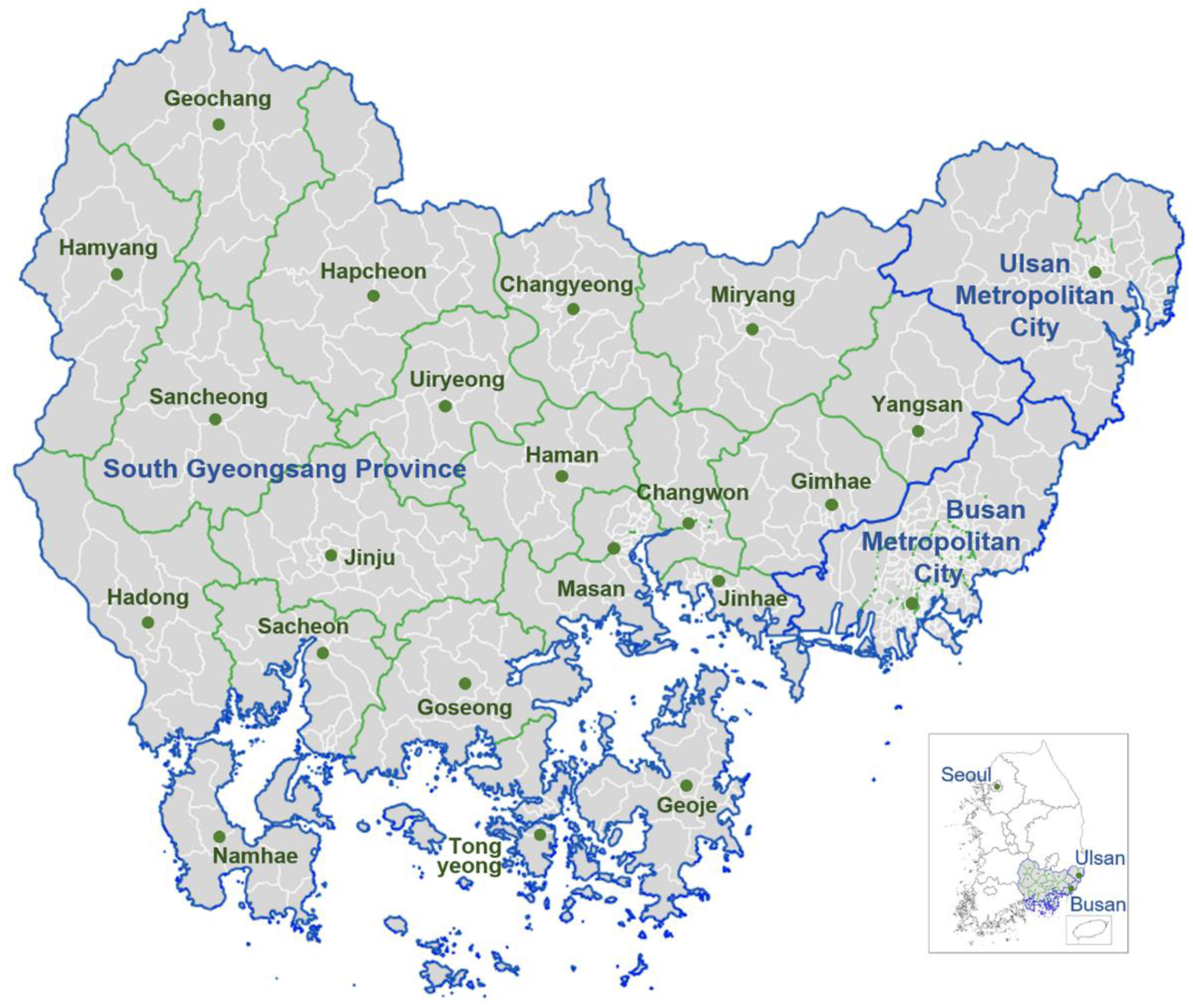
4. Study Area and Dataset
5. Results
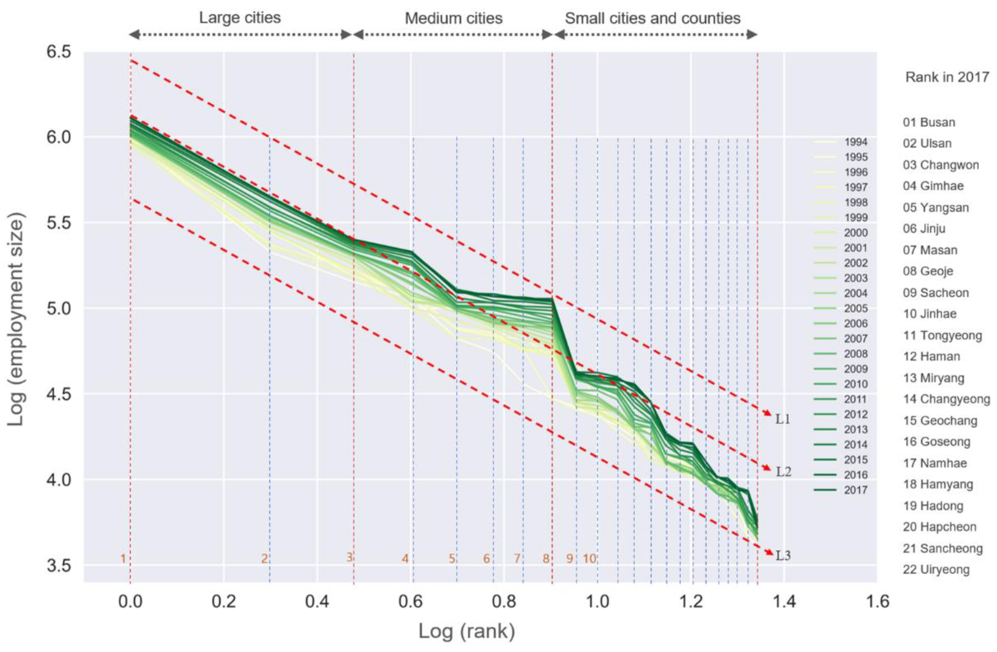
5.1. Zipf Scaling
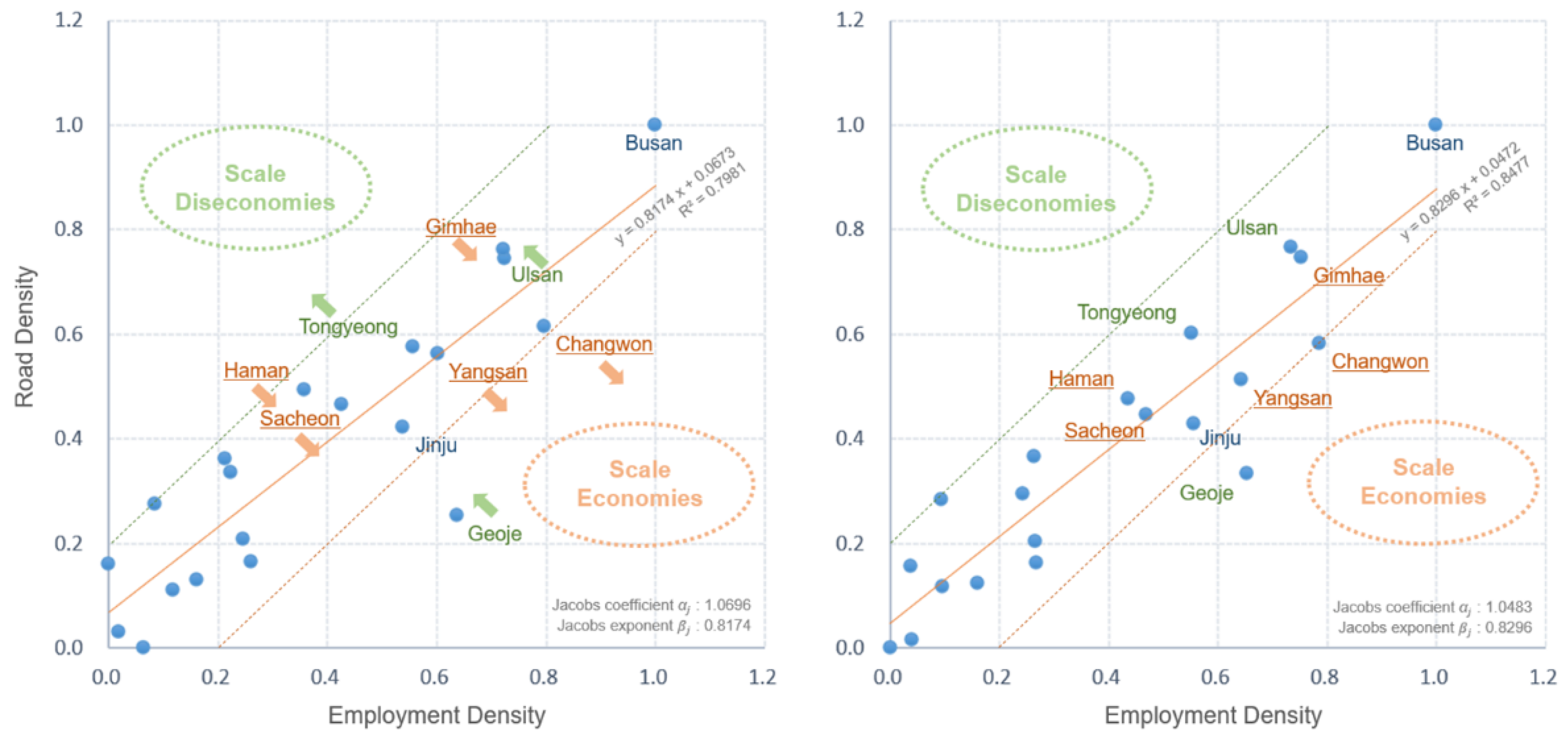
5.2. Jacobs Scaling
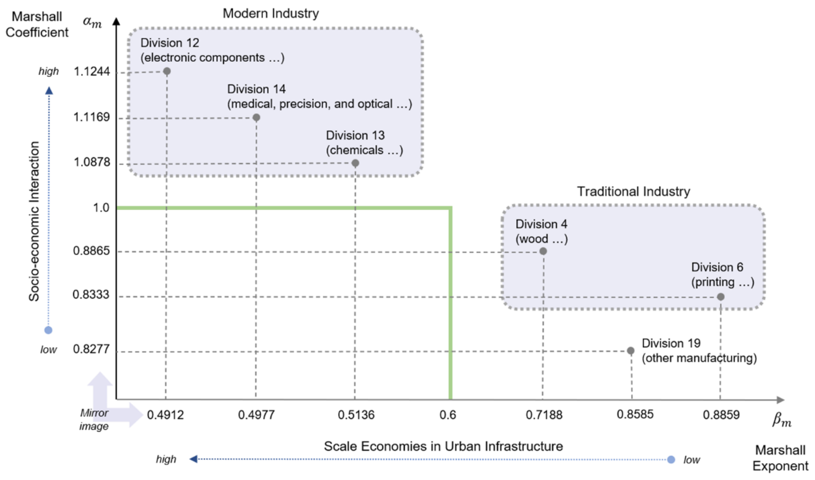
5.3. Marshall–Arrow–Romer Scaling
6. Discussion
6.1. Zipf Scaling
6.2. Jacobs Scaling
6.3. Marshall–Arrow–Romer Scaling
7. Summary
Author Contributions
Funding
Institutional Review Board Statement
Informed Consent Statement
Data Availability Statement
Acknowledgments
Conflicts of Interest
References
- Hwang, U.; Woo, M. Analysis of inter-relationships between urban decline and urban sprawl in city-regions of South Korea. Sustainability 2020, 12, 1656. [Google Scholar] [CrossRef] [Green Version]
- Ortiz-Moya, F.; Moreno, N. The incredible shrinking Japan. City 2016, 20, 880–903. [Google Scholar] [CrossRef]
- Yi, Z. Options for fertility policy transition in China. Popul. Dev. Rev. 2007, 33, 215–246. [Google Scholar] [CrossRef]
- Cheshire, P.C.; Hay, D.G. Urban Problems in Western Europe; Routledge: London, UK, 1989. [Google Scholar]
- Henderson, V.; Kuncoro, A.; Turner, M. Industrial development in cities. J. Pol. Econ. 1995, 103, 1067–1090. [Google Scholar] [CrossRef]
- De Groot, H.; Poot, J.; Smit, M.J. Agglomeration externalities, innovation and regional growth: Theoretical perspectives and meta-analysis. In Handbook of Regional Growth and Development Theories; Capello, R., Nijkamp, P., Eds.; Edward Elgar Publishing: Cheltenham, UK, 2009; pp. 256–281. [Google Scholar]
- Duranton, G.; Puga, D. Nursery cities: Urban diversity, process innovation, and the life cycle of products. Am. Econ. Rev. 2001, 91, 1454–1477. [Google Scholar] [CrossRef] [Green Version]
- Rosenthal, S.S.; Strange, W.C. Geography, industrial organization, and agglomeration. Rev. Econ. Stat. 2003, 85, 377–393. [Google Scholar] [CrossRef] [Green Version]
- Cooke, P. From technopoles to regional innovation systems: The evolution of localised technology development policy. Can. J. Reg. Sci. 2001, 24, 21–40. [Google Scholar]
- Harrison, B. Industrial districts: Old wine in new bottles? Reg. Stud. 1992, 26, 469–483. [Google Scholar] [CrossRef]
- Jacobs, J. The Economy of Cities; Vintage Book Company: New York, NY, USA, 1969. [Google Scholar]
- Rosental, S.S.; Strange, W.C. Evidence on the nature and source of agglomeration economies. In Handbook of Regional and Urban Economics: Cities and Geography, 4th ed.; Henderson, J.V., Thisse, J.F., Eds.; Elsevier: Amsterdam, The Netherlands, 2004. [Google Scholar]
- Glaeser, E. Triumph of the City: How Our Greatest Invention Makes Us Richer, Smarter, Greener, Healthier, and Happier; The Penguin Press: New York, NY, USA, 2012. [Google Scholar]
- Glaeser, E.L.; Gottlieb, J.D. The wealth of cities: Agglomeration economies and spatial equilibrium in the United States. J. Econ. Lit. 2009, 47, 983–1028. [Google Scholar] [CrossRef] [Green Version]
- Van Meeteren, M.; Neal, Z.; Derudder, B. Disentangling agglomeration and network externalities: A conceptual typology. Pap. Reg. Sci. 2016, 95, 61–80. [Google Scholar] [CrossRef] [Green Version]
- Arcaute, E.; Hatna, E.; Ferguson, P.; Youn, H.; Johansson, A.; Batty, M. Constructing cities, deconstructing scaling laws. J. R. Soc. Interface 2015, 12, 20140745. [Google Scholar] [CrossRef] [PubMed]
- Yang, J.; Ettema, D. Modelling the emergence of spatial patterns of economic activity. J. Artif. Soc. Soc. Simul. 2012, 15, 6. [Google Scholar] [CrossRef]
- Van Soest, D.P.; Gerking, S.; van Oort, F.G. Spatial impacts of agglomeration externalities. J. Reg. Sci. 2006, 46, 881–899. [Google Scholar] [CrossRef]
- Cottineau, C.; Finance, O.; Hatna, E.; Arcaute, E.; Batty, M. Defining urban clusters to detect agglomeration economies. Environ. Plan. B Urban Anal. City Sci. 2019, 46, 1611–1626. [Google Scholar] [CrossRef] [Green Version]
- Wilson, B. Metropolis: A History of the City, Humankind’s Greatest Invention; Jonathan Cape: London, UK, 2020. [Google Scholar]
- Openshaw, S.; Taylor, P.J. The modifiable areal unit problem. In Quantitative Geography: A British View; Wrigley, N., Bennett, R.J., Eds.; Routledge: London, UK, 1981. [Google Scholar]
- Openshaw, S. The Modifiable Areal Unit Problem; Geo Books: Norwich, UK, 1983. [Google Scholar]
- Reardon, S.F. A conceptual framework for measuring segregation and its association with population outcomes. In Methods in Social Epidemiology; Oakes, J.M., Kaufman, J.S., Eds.; Jossey-Bass: San Francisco, CA, USA, 2006; pp. 169–192. [Google Scholar]
- Wong, D.W.S.; Lasus, H.; Falk, R.F. Exploring the variability of segregation index D with scale and zonal systems: An analysis of thirty US cities. Environ. Plan. A 1999, 31, 507–522. [Google Scholar] [CrossRef]
- Amrhein, C.G.; Flowerdew, R. The effect of data aggregation on a Poisson regression model of Canadian migration. Environ. Plan. A 1992, 24, 1381–1391. [Google Scholar] [CrossRef]
- Andersson, M.; Klaesson, J.; Larsson, J.P. How local are spatial density externalities? Neighbourhood effects in agglomeration economies. Reg. Stud. 2016, 50, 1082–1095. [Google Scholar] [CrossRef]
- Briant, A.; Combes, P.-P.; Lafourcade, M. Dots to boxes: Do the size and shape of spatial units jeopardize economic geography estimations? J. Urban Econ. 2010, 67, 287–302. [Google Scholar] [CrossRef] [Green Version]
- Burger, M.J.; van Oort, F.G.; van der Knaap, G.A. A treatise on the geographical scale of agglomeration externalities and the modifiable areal unit problem. Sci. Reg. 2010, 9, 19–40. [Google Scholar]
- Wrigley, N. Revisiting the modifiable areal unit problem and the ecological fallacy. In Diffusing Geography: Essays for Peter Haggett; Cliff, A.D., Gould, P.R., Hoare, A.G., Thrift, N.J., Eds.; Blackwell Publishing: Cambridge, MA, USA, 1995; pp. 49–71. [Google Scholar]
- Ross, C.L. Megaregions: Planning for Global Competitiveness; Island Press: Washington, DC, USA, 2009. [Google Scholar]
- Rybski, D.; Arcaute, E.; Batty, M. Urban scaling laws. Environ. Plan. B 2019, 46, 1605–1610. [Google Scholar] [CrossRef]
- Lösch, A. The Economics of Location; Yale University Press: New Haven, CT, USA, 1954. [Google Scholar]
- Weber, A. Alfred Weber’s Theory of the Location of Industries; University of Chicago Press: Chicago, IL, USA, 1929. [Google Scholar]
- Batty, M. Fifty years of urban modelling: Macro statics to micro dynamics. In The Dynamics of Complex Urban Systems: An Interdisciplinary Approach; Albeverio, S., Andrey, D., Giordano, P., Vancheri, A., Eds.; Physica Verlag: Heidelberg, Germany, 2008; pp. 1–20. [Google Scholar]
- Schweitzer, F. Brownian Agents and Active Particles: Collective Dynamics in the Natural and Social Sciences; Springer: Berlin/Heidelberg, Germany, 2003. [Google Scholar]
- Bettencourt, L.M.A. The origins of scaling in cities. Science 2013, 340, 1438–1441. [Google Scholar] [CrossRef] [Green Version]
- Bettencourt, L.M.A.; Lobo, J.; Helbing, D.; Kühnert, C.; West, G.B. Growth, innovation, scaling, and the pace of life in cities. Proc. Natl Acad. Sci. USA 2007, 104, 7301–7306. [Google Scholar] [CrossRef] [PubMed] [Green Version]
- Ball, P. Critical Mass: How One Thing Leads to Another; Farrar, Straus & Giroux: New York, NY, USA, 2006. [Google Scholar]
- Zipf, G.K. Human Behavior and the Principle of Least Effort; Addison-Wesley: Cambridge, MA, USA, 1949. [Google Scholar]
- Jiang, B.; Jia, T. Zipf’s law for all the natural cities in the United States: A geospatial perspective. Int. J. Geogr. Inf. Sci. 2011, 25, 1269–1281. [Google Scholar] [CrossRef]
- Batty, M. Cities and Complexity: Understanding Cities with Cellular Automata, Agent-Based Models, and Fractals; The MIT Press: Cambridge, MA, USA, 2007. [Google Scholar]
- Rosen, K.T.; Resnick, M. The size distribution of cities: An examination of the Pareto law and primacy. J. Urban Econ. 1980, 8, 165–186. [Google Scholar] [CrossRef] [Green Version]
- Krugman, P. The Self Organizing Economy; Blackwell Publishers: Cambridge, MA, USA, 1996. [Google Scholar]
- Kühnert, C.; Helbing, D.; West, G.B. Scaling laws in urban supply networks. Phys. A 2006, 363, 96–103. [Google Scholar] [CrossRef]
- Sarkar, S.; Arcaute, E.; Hatna, E.; Alizadeh, T.; Searle, G.; Batty, M. Evidence for localization and urbanization economies in urban scaling. R. Soc. Open Sci. 2020, 7, 191638. [Google Scholar] [CrossRef] [Green Version]
- West, G. Scale: The Universal Laws of Life, Growth, and Death in Organisms, Cities, and Companies; Penguin Press: New York, NY, USA, 2018. [Google Scholar]
- Staber, U. Spatial proximity and firm survival in a declining industrial district: The case of knitwear firms in Baden-Württemberg. Reg. Stud. 2001, 35, 329–341. [Google Scholar] [CrossRef]
- Feldman, M.P. The new economics of innovation, spillovers and agglomeration: A review of empirical studies. Econ. Innov. New Technol. 1999, 8, 5–25. [Google Scholar] [CrossRef]
- Frenken, K.; van Oort, F.G.; Verburg, T.; Boschma, R.A. Variety and regional economic growth in the Netherlands. In Research Series. Final Report to the Ministry of Economic Affairs; Ministry of Economic Affairs: The Hague, The Netherlands, 2004. [Google Scholar]
- Ning, L.; Wang, F.; Li, J. Urban innovation, regional externalities of foreign direct investment and industrial agglomeration: Evidence from Chinese cities. Res. Policy 2016, 45, 830–843. [Google Scholar] [CrossRef]
- Rosenthal, S.S.; Strange, W.C. The determinants of agglomeration. J. Urban Econ. 2001, 50, 191–229. [Google Scholar] [CrossRef] [Green Version]
- Park, B. The territorial politics of regulation under state capitalism: Regional parties and the politics of local economic development in South Korea. Space Pol. 2005, 9, 237–259. [Google Scholar] [CrossRef]
- Park, B. Uneven development, inter-scalar tensions, and the politics of decentralization in South Korea. Int. J. Urban Reg. Res. 2008, 32, 40–59. [Google Scholar] [CrossRef]
- Duffie, N.A. Heterarchical control of highly distributed manufacturing systems. Int. J. Comput. Integr. Manuf. 1996, 9, 270–281. [Google Scholar] [CrossRef]
- Boonstra, B.; Boelens, L. Self-organization in urban development: Towards a new perspective on spatial planning. Urban Res. Pract. 2011, 4, 99–122. [Google Scholar] [CrossRef]
- Fujita, M.; Krugman, P.; Mori, T. On the evolution of hierarchical urban systems. Eur. Econ. Rev. 1999, 43, 209–251. [Google Scholar] [CrossRef]
- Hanley, Q.S.; Lewis, D.; Ribeiro, H.V. Correction: Rural to urban population density scaling of crime and property Transactions in English and Welsh Parliamentary Constituencies. Transactions of the in English and Welsh Parliamentary Constituencies. Transactions of the in English and Welsh Parliamentary Constituencies. PLoS ONE 2016, 11, e0167605. [Google Scholar] [CrossRef] [Green Version]
- Sotomayor-Gómez, B.; Samaniego, H. City limits in the age of smartphones and urban scaling. Comput. Environ. Urban Syst. 2020, 79, 101423. [Google Scholar] [CrossRef]
- Devereux, M.P.; Griffith, R.; Simpson, H. The geographic distribution of production activity in the UK. Reg. Sci. Urban Econ. 2004, 34, 533–564. [Google Scholar] [CrossRef]
- Ellison, G.; Glaeser, E.L.; Kerr, W.R. What causes industry agglomeration? Evidence from Coagglomeration Patterns. Am. Econ. Rev. 2010, 100, 1195–1213. [Google Scholar] [CrossRef] [Green Version]
- Mukkala, K. Agglomeration economies in the Finnish manufacturing sector. Appl. Econ. 2004, 36, 2419–2427. [Google Scholar] [CrossRef] [Green Version]
- Wennberg, K.; Lindqvist, G. The effect of clusters on the survival and performance of new firms. Small Bus. Econ. 2010, 34, 221–241. [Google Scholar] [CrossRef]


| Type | Division | Name | 2006 | |||||
|---|---|---|---|---|---|---|---|---|
| β | p > |t| | ln α | p > |t| | α | adj. R² | |||
| Traditional Industry | 1 | Food products | 0.712 | 0.000 | −0.029 | 0.614 | 0.971 | 0.637 |
| 2 | Textiles except apparel | 0.599 | 0.000 | −0.040 | 0.546 | 0.961 | 0.579 | |
| 3 | Wearing apparel, clothing | 0.849 | 0.000 | −0.104 | 0.134 | 0.901 | 0.648 | |
| 4 | Wood and products of wood | 0.719 | 0.000 | −0.120 | 0.075 | 0.886 | 0.685 | |
| 5 | Pulp, paper and paper products | 0.383 | 0.002 | 0.108 | 0.070 | 1.115 | 0.392 | |
| 6 | Printing and reproduction | 0.886 | 0.000 | −0.182 | 0.011 | 0.833 | 0.736 | |
| 7 | Rubber and plastic products | 0.436 | 0.001 | 0.073 | 0.211 | 1.076 | 0.469 | |
| 8 | Other non-metallic minerals | 0.648 | 0.004 | −0.126 | 0.311 | 0.882 | 0.339 | |
| 9 | Furniture | 0.592 | 0.000 | −0.022 | 0.707 | 0.978 | 0.623 | |
| Modern Industry | 10 | Basic metals | 0.412 | 0.000 | 0.106 | 0.050 | 1.112 | 0.482 |
| 11 | Fabricated metal products | 0.618 | 0.000 | −0.082 | 0.263 | 0.921 | 0.585 | |
| 12 | Electronic components | 0.491 | 0.000 | 0.117 | 0.008 | 1.124 | 0.635 | |
| 13 | Chemicals and chemical | 0.514 | 0.000 | 0.084 | 0.070 | 1.088 | 0.623 | |
| 14 | Medical, precision and optical | 0.498 | 0.000 | 0.111 | 0.019 | 1.117 | 0.590 | |
| 15 | Electrical equipment | 0.550 | 0.000 | 0.020 | 0.707 | 1.020 | 0.622 | |
| 16 | Other machinery and equipment | 0.457 | 0.000 | 0.039 | 0.475 | 1.040 | 0.569 | |
| 17 | Motor vehicles, trailers | 0.376 | 0.001 | 0.073 | 0.247 | 1.076 | 0.414 | |
| 18 | Other transport equipment | 0.407 | 0.002 | 0.068 | 0.309 | 1.071 | 0.379 | |
| others | 19 | Other manufacturing | 0.859 | 0.000 | −0.189 | 0.026 | 0.828 | 0.654 |
| Type | Division | Name | 2011 | |||||
|---|---|---|---|---|---|---|---|---|
| β | p > |t| | ln α | p > |t| | α | adj. R² | |||
| Traditional Industry | 1 | Food products | 0.685 | 0.000 | −0.057 | 0.419 | 0.945 | 0.563 |
| 2 | Textiles except apparel | 0.525 | 0.000 | −0.010 | 0.884 | 0.990 | 0.477 | |
| 3 | Wearing apparel, clothing | 0.726 | 0.000 | −0.015 | 0.809 | 0.985 | 0.559 | |
| 4 | Wood and products of wood | 0.534 | 0.000 | 0.010 | 0.856 | 1.011 | 0.572 | |
| 5 | Pulp, paper and paper products | 0.388 | 0.003 | 0.090 | 0.159 | 1.094 | 0.363 | |
| 6 | Printing and reproduction | 0.808 | 0.000 | −0.127 | 0.068 | 0.881 | 0.674 | |
| 7 | Rubber and plastic products | 0.450 | 0.000 | 0.069 | 0.215 | 1.072 | 0.505 | |
| 8 | Other non-metallic minerals | 0.688 | 0.001 | −0.121 | 0.223 | 0.886 | 0.454 | |
| 9 | Furniture | 0.591 | 0.000 | −0.031 | 0.601 | 0.970 | 0.621 | |
| Modern Industry | 10 | Basic metals | 0.403 | 0.001 | 0.060 | 0.350 | 1.061 | 0.422 |
| 11 | Fabricated metal products | 0.681 | 0.000 | −0.212 | 0.072 | 0.809 | 0.480 | |
| 12 | Electronic components | 0.520 | 0.000 | 0.105 | 0.016 | 1.111 | 0.650 | |
| 13 | Chemicals and chemical | 0.515 | 0.000 | 0.065 | 0.168 | 1.068 | 0.622 | |
| 14 | Medical, precision and optical | 0.526 | 0.000 | 0.082 | 0.075 | 1.085 | 0.626 | |
| 15 | Electrical equipment | 0.489 | 0.000 | 0.069 | 0.176 | 1.071 | 0.570 | |
| 16 | Other machinery and equipment | 0.449 | 0.000 | 0.035 | 0.557 | 1.035 | 0.517 | |
| 17 | Motor vehicles, trailers | 0.368 | 0.002 | 0.064 | 0.334 | 1.066 | 0.387 | |
| 18 | Other transport equipment | 0.400 | 0.004 | 0.051 | 0.486 | 1.053 | 0.336 | |
| others | 19 | Other manufacturing | 0.843 | 0.000 | −0.071 | 0.081 | 0.932 | 0.835 |
| Type | Division | Name | 2017 | |||||
|---|---|---|---|---|---|---|---|---|
| β | p > |t| | ln α | p > |t| | α | adj. R² | |||
| Traditional Industry | 1 | Food products | 0.812 | 0.000 | −0.154 | 0.031 | 0.857 | 0.671 |
| 2 | Textiles except apparel | 0.515 | 0.000 | −0.008 | 0.891 | 0.992 | 0.543 | |
| 3 | Wearing apparel, clothing | 0.599 | 0.000 | 0.024 | 0.675 | 1.025 | 0.499 | |
| 4 | Wood and products of wood | 0.433 | 0.001 | 0.030 | 0.636 | 1.031 | 0.425 | |
| 5 | Pulp, paper and paper products | 0.365 | 0.004 | 0.070 | 0.265 | 1.073 | 0.346 | |
| 6 | Printing and reproduction | 0.686 | 0.000 | −0.073 | 0.193 | 0.930 | 0.681 | |
| 7 | Rubber and plastic products | 0.395 | 0.002 | 0.056 | 0.358 | 1.058 | 0.396 | |
| 8 | Other non-metallic minerals | 0.575 | 0.001 | −0.057 | 0.489 | 0.945 | 0.429 | |
| 9 | Furniture | 0.676 | 0.000 | −0.123 | 0.102 | 0.884 | 0.597 | |
| Modern Industry | 10 | Basic metals | 0.344 | 0.005 | 0.058 | 0.392 | 1.059 | 0.328 |
| 11 | Fabricated metal products | 0.504 | 0.001 | −0.072 | 0.410 | 0.931 | 0.420 | |
| 12 | Electronic components | 0.455 | 0.000 | 0.105 | 0.021 | 1.111 | 0.557 | |
| 13 | Chemicals and chemical | 0.491 | 0.000 | 0.026 | 0.644 | 1.026 | 0.517 | |
| 14 | Medical, precision and optical | 0.458 | 0.000 | 0.049 | 0.368 | 1.050 | 0.497 | |
| 15 | Electrical equipment | 0.418 | 0.000 | 0.065 | 0.224 | 1.067 | 0.486 | |
| 16 | Other machinery and equipment | 0.394 | 0.003 | 0.000 | 0.997 | 1.000 | 0.369 | |
| 17 | Motor vehicles, trailers | 0.313 | 0.006 | 0.071 | 0.277 | 1.074 | 0.319 | |
| 18 | Other transport equipment | 0.360 | 0.007 | 0.050 | 0.482 | 1.052 | 0.304 | |
| others | 19 | Other manufacturing | 0.812 | 0.000 | −0.241 | 0.014 | 0.786 | 0.611 |
Publisher’s Note: MDPI stays neutral with regard to jurisdictional claims in published maps and institutional affiliations. |
© 2022 by the authors. Licensee MDPI, Basel, Switzerland. This article is an open access article distributed under the terms and conditions of the Creative Commons Attribution (CC BY) license (https://creativecommons.org/licenses/by/4.0/).
Share and Cite
Yang, J.-H.; Nam, K.-W. Modelling the Relationship of Infrastructure and Externalities Using Urban Scaling. Sustainability 2022, 14, 5091. https://doi.org/10.3390/su14095091
Yang J-H, Nam K-W. Modelling the Relationship of Infrastructure and Externalities Using Urban Scaling. Sustainability. 2022; 14(9):5091. https://doi.org/10.3390/su14095091
Chicago/Turabian StyleYang, Jung-Hun, and Kwang-Woo Nam. 2022. "Modelling the Relationship of Infrastructure and Externalities Using Urban Scaling" Sustainability 14, no. 9: 5091. https://doi.org/10.3390/su14095091
APA StyleYang, J.-H., & Nam, K.-W. (2022). Modelling the Relationship of Infrastructure and Externalities Using Urban Scaling. Sustainability, 14(9), 5091. https://doi.org/10.3390/su14095091