China’s Public Firms’ Attitudes towards Environmental Protection Based on Sentiment Analysis and Random Forest Models
Abstract
:1. Introduction
2. Materials and Methods
2.1. Workflow
2.2. NLP
2.3. Sentiment Analysis
2.4. Random Forests
2.5. Data
3. Results and Discussion
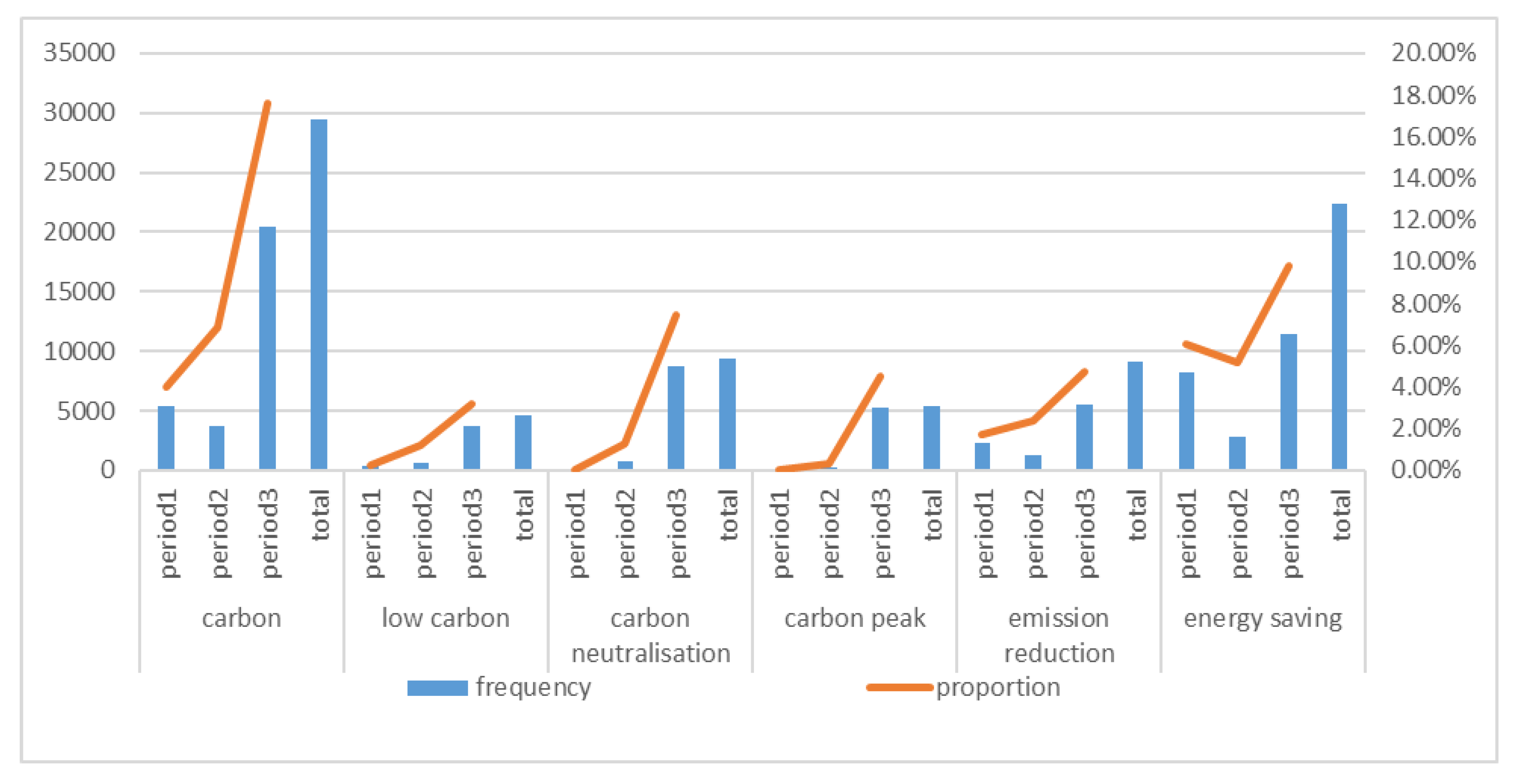
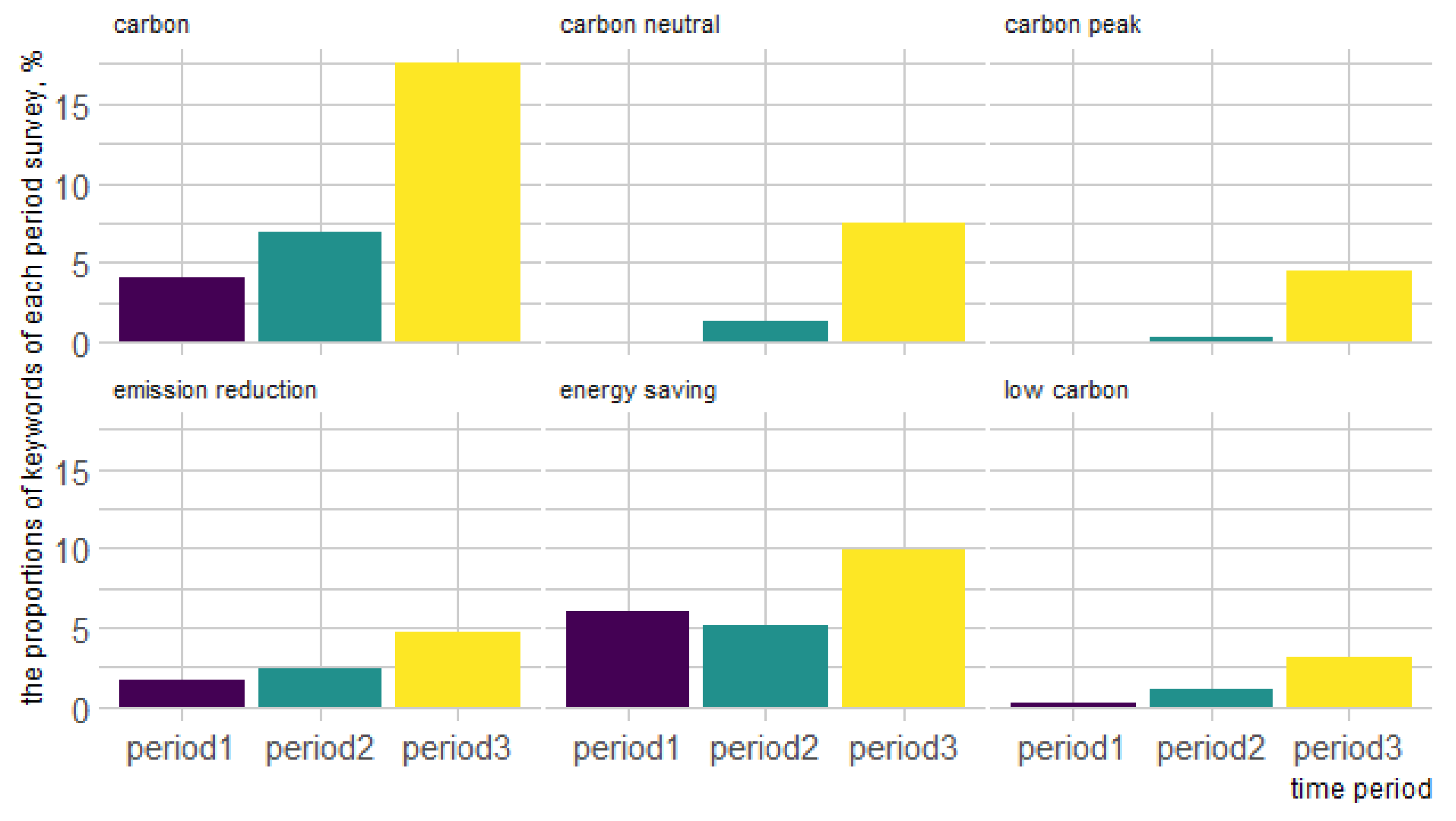
3.1. Descriptive Statistical Results of the Raw Data
3.2. Data Pre-Processing
3.3. Sentiment Weight and Characteristics
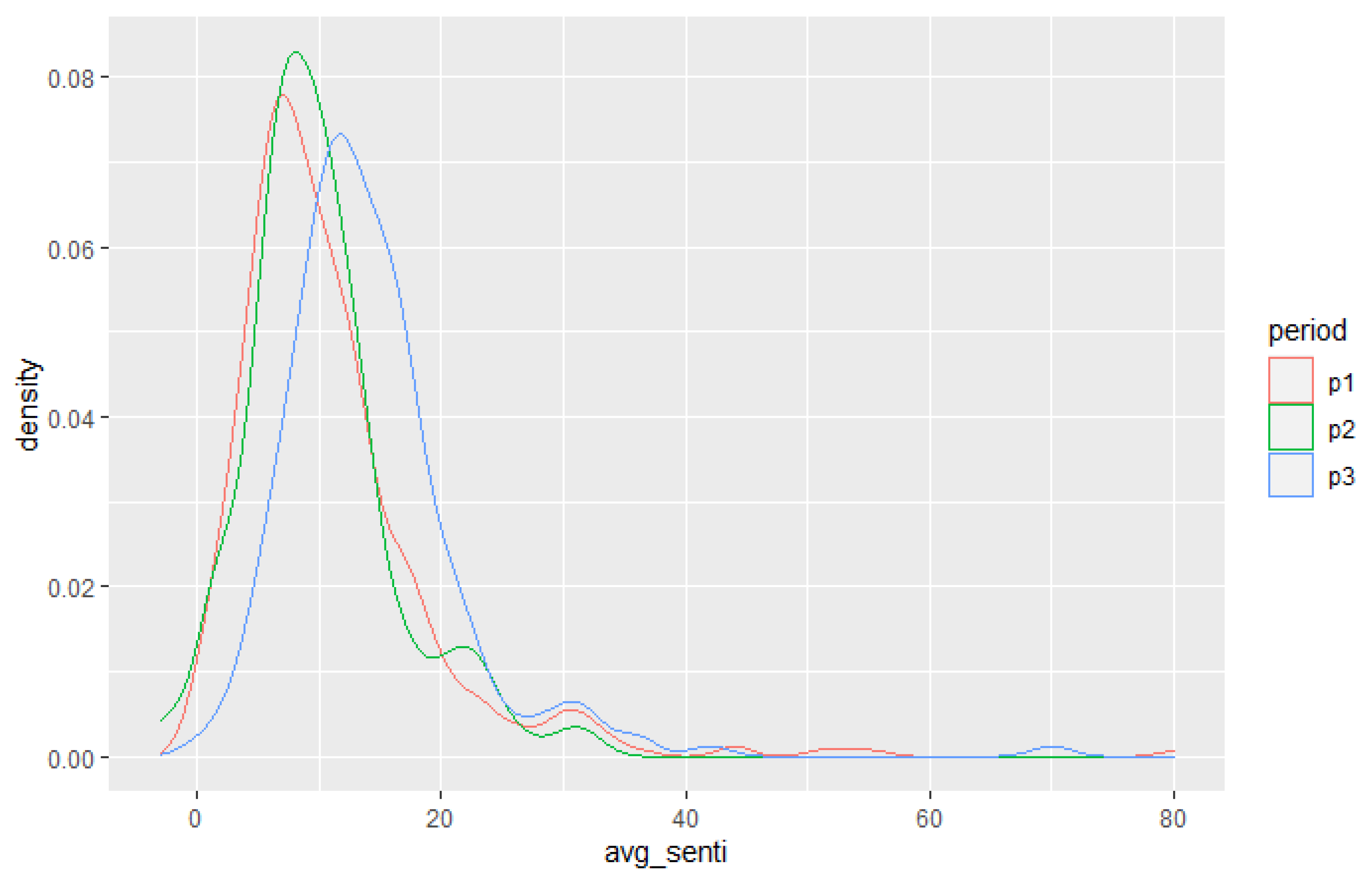
3.3.1. The Result of the Sentiment Analysis and its Distribution
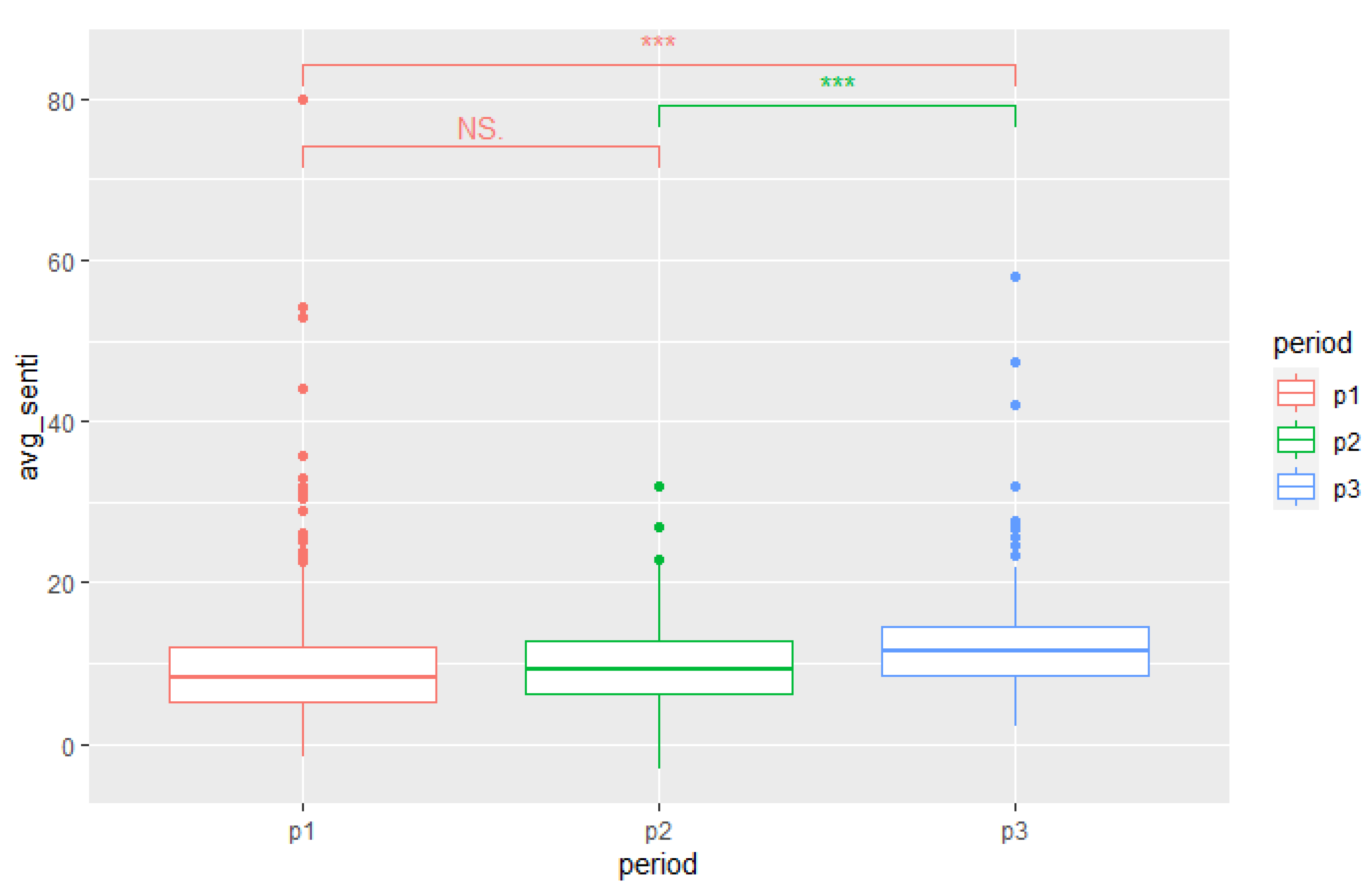
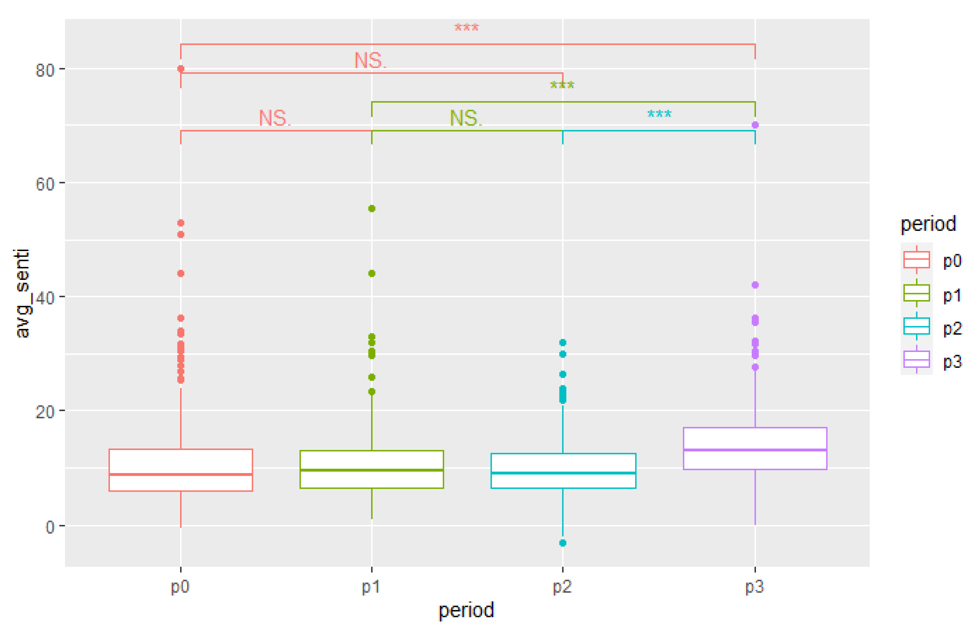
3.3.2. The Group Differences in Sentiment Weight
3.4. Predictive Models of Firms’ Sentiment Weights and Stock Data Based on Advanced Tree Models
3.4.1. Model l
3.4.2. Model 2
3.4.3. Stepwise Feature Selection
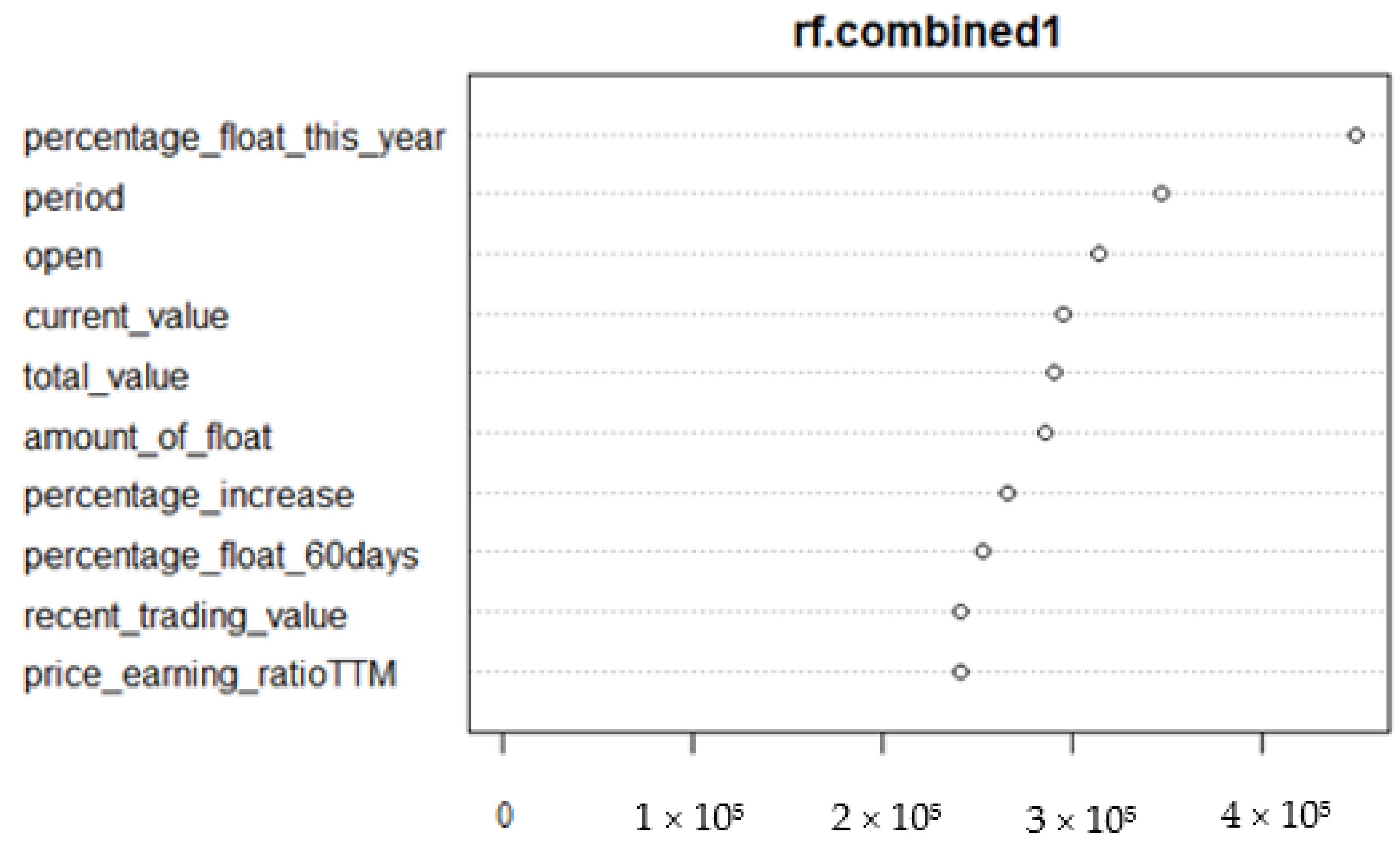
3.4.4. Model 3
3.4.5. Model 4
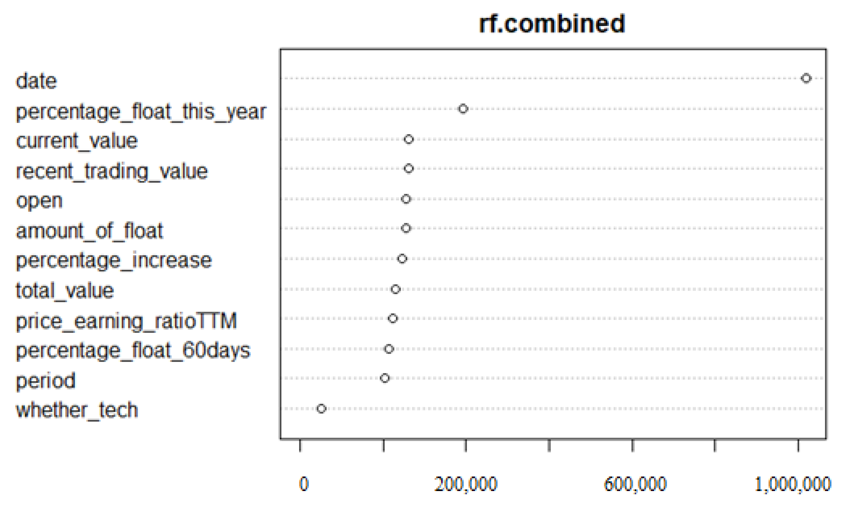
3.4.6. Prediction and Model Assessment
4. Conclusions
- There was a significant increase in firms’ attitudes towards carbon reduction and environmental protection after the “Double Carbon” goal was incorporated into the government’s work report and consequent relevant policies were added, but the same significant increase was not found after the goal was proposed.
- A strong significance could be observed in the differences in attitude among the industries. A total of 3122 of the 4560 possible pairs for comparison showed a strong significance in the differences in industries’ attitudes towards carbon reduction and environmental protection.
- The influence of COVID-19 on attitudes was not observed.
- Then, in the linear regression models, we observed that:
- Whether a firm is in a technology industry significantly influences the firm’s attitude.
- Other significantly related variables were stock value, the increase in stock value since the start of the year, and stock data.
- COVID-19 significantly influenced firms’ attitudes towards carbon reduction and environmental protection, which was different from the findings in the verification of the significance of group differences.
- A goal with consequent specific policies can raise the positive attitudes of firms toward carbon reduction topics, but not the goal alone.
- Firms’ attitudes toward ecological topics are different from industry to industry, which means that there are different needs and situations in the trend of carbon reduction from industry to industry. Detailed policies with differentiation will be more suitable.
- COVID-19 influences firms’ attitudes toward carbon reduction and environmental protection, calling back the classic dilemma or trilemma of economic growth, carbon reduction, and a third factor, such as energy consumption or epidemic controls today.
Author Contributions
Funding
Institutional Review Board Statement
Informed Consent Statement
Data Availability Statement
Acknowledgments
Conflicts of Interest
Appendix A
| Term | Estimate | Std.Error | t Value | p. Value | Signif Codes | |
|---|---|---|---|---|---|---|
| 1 | (intercept) | 122.8467 | 14.49061 | 8.477671 | 2.36 × 10⁻¹⁷ | *** |
| 2 | date | −0.00641 | 0.000802 | −7.99338 | 1.34 × 10⁻¹⁵ | *** |
| 3 | current_value | −1.08527 | 0.101149 | −10.7294 | 7.91 × 10⁻²⁷ | *** |
| 4 | percentage of increase | 0.620066 | 0.039568 | 15.6709 | 3.22 × 10−55 | *** |
| 5 | amount of float | 0.803083 | 0.116003 | 6.922919 | 4.48 × 10⁻¹² | *** |
| 6 | volume | 2.55 × 10⁻⁹ | 6.16 × 10⁻⁹ | 0.414112 | 0.678794 | *** |
| 7 | recent trading volume | −0.0001 | 4.80 × 10⁻⁵ | −2.18349 | 0.029005 | |
| 8 | open | 1.084942 | 0.10173 | 10.66495 | 1.58 × 10⁻²⁶ | * |
| 9 | price–earnings ratio.TTM. | −0.00116 | 0.000548 | −2.1149 | 0.034443 | *** |
| 10 | total value | 8.12 × 10⁻¹² | 1.67 × 10⁻¹² | 4.871945 | 1.11 × 10⁻⁶ | * |
| 11–105 industry, compare to white household appliances | semiconductors | −1.32583 | 0.932814 | −1.42132 | 0.15523 | *** |
| glass | 17.30774 | 4.51258 | 3.835443 | 0.000125 | ||
| animal husbandry | −2.84401 | 0.881095 | −3.22782 | 0.001248 | *** | |
| ship and marine equipment | 7.157058 | 5.274547 | 1.356905 | 0.174817 | ** | |
| motor | 0.878144 | 1.1123 | 0.789484 | 0.429833 | ||
| electricity | 0.273886 | 0.990088 | 0.276628 | 0.782067 | ||
| power supply | 3.588364 | 0.908556 | 3.949524 | 7.84 × 10⁻⁵ | *** | |
| electronic devices | −4.19587 | 1.165698 | −3.59945 | 0.000319 | *** | |
| electronic equipment manufacturing | 2.439399 | 0.810315 | 3.010434 | 0.00261 | ** | |
| electronic components | −0.6249 | 0.955577 | −0.65395 | 0.513147 | ||
| real estate development | 4.541732 | 2.479098 | 1.83201 | 0.066956 | . | |
| textiles | −1.77311 | 4.728651 | −0.37497 | 0.707684 | ||
| non-bank finance | 0.707548 | 1.879389 | 0.376478 | 0.706563 | ||
| clothing and home textiles | −3.80677 | 1.030464 | −3.69423 | 0.000221 | *** | |
| steel structures | −0.10154 | 0.836296 | −0.12141 | 0.903363 | ||
| steel | 3.011207 | 0.846367 | 3.557804 | 0.000374 | *** | |
| port shipping | 10.49783 | 2.23662 | 4.693615 | 2.69 × 10⁻⁶ | *** | |
| road rail | 2.25131 | 2.450983 | 0.918533 | 0.358344 | ||
| optoelectronic device | −4.2997 | 1.129387 | −3.80711 | 0.000141 | *** | |
| broadcasting | −2.6028 | 8.556085 | −0.3042 | 0.760973 | ||
| rail transit equipment | 50.76793 | 5.629349 | 9.018438 | 1.97 × 10⁻¹⁹ | *** | |
| precious metals | 9.219086 | 8.562859 | 1.076636 | 0.281648 | ||
| aerospace equipment | −6.87912 | 1.93049 | −3.56341 | 0.000366 | *** | |
| aviation airport | 4.404922 | 3.31229 | 1.329872 | 0.183566 | ||
| synthetic fiber and resin | 10.09359 | 0.884497 | 11.41167 | 3.98 × 10⁻³⁰ | *** | |
| internet service | 5.966019 | 1.417503 | 4.208824 | 2.57 × 10⁻⁵ | *** | |
| internet technology | 0.699786 | 1.940025 | 0.36071 | 0.718318 | ||
| internet business | −2.54472 | 7.420536 | −0.34293 | 0.731653 | ||
| fertilizers and pesticides | −0.88422 | 0.850499 | −1.03965 | 0.298507 | ||
| new chemical materials | 17.6047 | 0.928078 | 18.969 | 5.81 × 10−80 | *** | |
| chemical materials | 2.414427 | 0.819692 | 2.945528 | 0.003226 | ** | |
| chemicals | 5.166898 | 0.796451 | 6.487399 | 8.81 × 10⁻¹¹ | *** | |
| chemical and pharmaceutical | −1.78932 | 0.919407 | −1.94617 | 0.051639 | . | |
| environmental protection | 21.78406 | 0.951113 | 22.90376 | 1.64 × 10−115 | *** | |
| robots | −1.46364 | 0.923671 | −1.58459 | 0.113066 | ||
| basic metal | 0.200088 | 0.838384 | 0.23866 | 0.811371 | ||
| infrastructure | 0.556408 | 1.685168 | 0.330179 | 0.741266 | ||
| computer software | 15.19635 | 0.954484 | 15.92101 | 6.22 × 10−57 | *** | |
| computer hardware | 3.747518 | 1.074415 | 3.487961 | 0.000487 | *** | |
| furniture | 0.243515 | 1.168628 | 0.208377 | 0.834935 | ||
| building construction | 17.80526 | 0.9709 | 18.33893 | 7.05 × 10−75 | *** | |
| education | −1.79009 | 6.644787 | −0.2694 | 0.787624 | ||
| new metal and non-metal materials | 6.083196 | 0.850658 | 7.151168 | 8.72 × 10⁻¹³ | *** | |
| metal products | −4.60701 | 0.828141 | −5.56307 | 2.66 × 10⁻⁸ | *** | |
| forestry | 3.114934 | 4.517578 | 0.689514 | 0.490503 | ||
| retail | 1.407416 | 4.511864 | 0.311937 | 0.75509 | ||
| trading | −3.13583 | 1.604586 | −1.95429 | 0.050672 | . | |
| coal | 1.563853 | 1.48919 | 1.050136 | 0.293661 | ||
| refractory | 14.41566 | 1.477046 | 9.759788 | 1.75 × 10⁻²² | *** | |
| agriculture | −4.29808 | 2.232262 | −1.92543 | 0.054181 | . | |
| print media | 2.806752 | 14.7815 | 0.189883 | 0.849402 | ||
| other electrical equipment | 3.493211 | 1.24306 | 2.810171 | 0.004953 | ** | |
| other home appliances | 1.133201 | 1.823094 | 0.621581 | 0.53422 | ||
| other building materials | −0.18492 | 0.978066 | −0.18907 | 0.85004 | ||
| other delivery equipment | 0.859954 | 1.894778 | 0.453855 | 0.649935 | ||
| other light industry | −0.46941 | 5.272863 | −0.08902 | 0.929063 | ||
| car | 1.765503 | 0.784958 | 2.249169 | 0.024506 | * | |
| gas | 0.629026 | 1.605851 | 0.391709 | 0.695275 | ||
| commercial property management | −0.98464 | 4.160513 | −0.23666 | 0.81292 | ||
| biomedicine | −4.41707 | 2.675452 | −1.65096 | 0.098753 | . | |
| petroleum gas | 6.115942 | 0.941699 | 6.49458 | 8.40 × 10⁻¹¹ | *** | |
| food | −3.0498 | 0.971268 | −3.14002 | 0.00169 | ** | |
| audiovisual equipment | 6.564379 | 1.479641 | 4.436468 | 9.16 × 10⁻⁶ | *** | |
| transmission and transformation equipment | 2.571072 | 0.960262 | 2.677469 | 0.00742 | ** | |
| cement | 2.756316 | 1.347438 | 2.045597 | 0.040801 | * | |
| water affairs | 2.879128 | 1.696806 | 1.696793 | 0.089742 | . | |
| ceramics | 6.746263 | 1.543292 | 4.371346 | 1.24 × 10⁻⁵ | *** | |
| iron ore | 6.121013 | 5.631601 | 1.086904 | 0.277084 | ||
| railway equipment | 5.180382 | 2.677895 | 1.934498 | 0.053058 | . | |
| communication devices | 3.312028 | 1.418248 | 2.335295 | 0.019532 | * | |
| general equipment | 1.097738 | 0.770044 | 1.425552 | 0.154004 | ||
| satellite applications | 2.709181 | 1.886708 | 1.43593 | 0.151028 | ||
| entertainment supplies | −2.35357 | 2.753838 | −0.85465 | 0.392749 | ||
| logistics | −1.19681 | 1.069861 | −1.11866 | 0.263291 | ||
| rare metals | −1.58956 | 1.16583 | −1.36346 | 0.172743 | ||
| rubber products | 2.218447 | 1.117255 | 1.985623 | 0.047081 | * | |
| consumer electronics | −3.93873 | 1.951649 | −2.01816 | 0.04358 | * | |
| home appliances | 2.522429 | 1.246603 | 2.023442 | 0.043033 | * | |
| leisure service | 0.435217 | 6.645008 | 0.065495 | 0.94778 | ||
| medical service | −4.71585 | 2.986223 | −1.5792 | 0.114296 | ||
| medical instruments | −4.50512 | 0.998439 | −4.51216 | 6.43 × 10⁻⁶ | *** | |
| pharmaceutical business | −6.10541 | 1.505683 | −4.05491 | 5.02 × 10⁻⁵ | *** | |
| banking | −3.27578 | 1.567455 | −2.08988 | 0.036634 | * | |
| drinks | −2.36368 | 4.164547 | −0.56757 | 0.570329 | ||
| marketing service | 1.954179 | 2.424267 | 0.806091 | 0.420194 | ||
| movies and animation | −4.28238 | 4.328788 | −0.98928 | 0.322531 | ||
| fishery | −1.3077 | 8.590432 | −0.15223 | 0.879008 | ||
| paper printing | 1.610445 | 0.896266 | 1.796838 | 0.072367 | . | |
| lighting devices | 2.220598 | 1.615952 | 1.374173 | 0.169394 | ||
| traditional Chinese medicine production | −4.44179 | 1.487589 | −2.9859 | 0.002829 | ** | |
| jewelry | −7.88081 | 3.236608 | −2.4349 | 0.014899 | * | |
| professional service | 8.09088 | 0.875021 | 9.246493 | 2.41 × 10⁻²⁰ | *** | |
| professional setting | −1.25212 | 0.794771 | −1.57545 | 0.11516 | ||
| decoration | 2.726903 | 1.62272 | 1.680452 | 0.092876 | . | |
| comprehensive | 1.854743 | 1.557577 | 1.190787 | 0.233743 | ||
| 106 | percentage of float in 60 days | −0.03486 | 0.003465 | −10.0612 | 8.63 × 10⁻²⁴ | *** |
| 107 | percentage of float in this year | 0.015725 | 0.000851 | 18.47594 | 5.72 × 10−76 | *** |
| periods 108–110, compare to p0 | periodp1 | 2.419141 | 0.353387 | 6.845588 | 7.70 × 10⁻¹² | *** |
| periodp2 | 4.221345 | 0.487625 | 8.656947 | 4.98 × 10⁻¹⁸ | *** | |
| periodp3 | 7.633121 | 0.617796 | 12.35541 | 5.11 × 10⁻³⁵ | *** |
| Name | Whether_Tech | |
|---|---|---|
| 1 | banking | 0 |
| 2 | glass | −1 |
| 3 | audiovisual equipment | 1 |
| 4 | other building materials | −1 |
| 5 | electricity | −1 |
| 6 | trading | 0 |
| 7 | environmental protection | 1 |
| 8 | real estate development | −1 |
| 9 | metal products | −1 |
| 10 | animal husbandry | −1 |
| 11 | electronic devices | 1 |
| 12 | building construction | −1 |
| 13 | basic metal | −1 |
| 14 | commercial property management | 0 |
| 15 | electronic components | 1 |
| 16 | chemical and pharmaceutical | 1 |
| 17 | professional setting | 1 |
| 18 | synthetic fiber and resin | −1 |
| 19 | white goods | −1 |
| 20 | car | 1 |
| 21 | transmission and transformation equipment | −1 |
| 22 | cement | −1 |
| 23 | gas | −1 |
| 24 | chemical materials | −1 |
| 25 | internet service | 1 |
| 26 | logistics | −1 |
| 27 | road rail | −1 |
| 28 | paper printing | −1 |
| 29 | infrastructure | −1 |
| 30 | port shipping | −1 |
| 31 | new metal and non-metal materials | 1 |
| 32 | food | −1 |
| 33 | general equipment | −1 |
| 34 | traditional Chinese medicine production | 1 |
| 35 | water affairs | −1 |
| 36 | coal | −1 |
| 37 | fertilizers and pesticides | −1 |
| 38 | petroleum gas | −1 |
| 39 | drinks | −1 |
| 40 | rubber products | −1 |
| 41 | power supply | −1 |
| 42 | forestry | −1 |
| 43 | medical service | 0 |
| 44 | non-bank finance | 0 |
| 45 | steel | −1 |
| 46 | rare metals | 1 |
| 47 | aerospace equipment | 1 |
| 48 | professional service | 0 |
| 49 | retail | 0 |
| 50 | biomedicine | 1 |
| 51 | new chemical materials | 1 |
| 52 | comprehensive | −1 |
| 53 | textile | −1 |
| 54 | chemicals | −1 |
| 55 | agriculture | −1 |
| 56 | broadcasting | 0 |
| 57 | motors | −1 |
| 58 | railway equipment | −1 |
| 59 | computer hardware | 1 |
| 60 | computer software | 1 |
| 61 | pharmaceutical business | 0 |
| 62 | electronic equipment manufacturing | 1 |
| 63 | iron ore | −1 |
| 64 | clothing and home textiles | −1 |
| 65 | decoration | −1 |
| 66 | refractory | −1 |
| 67 | semiconductors | 1 |
| 68 | communication devices | 1 |
| 69 | other delivery equipment | −1 |
| 70 | marketing service | 0 |
| 71 | steel structures | −1 |
| 72 | precious metals | −1 |
| 73 | leisure service | 0 |
| 74 | ceramics | −1 |
| 75 | education | 0 |
| 76 | movies and animation | 0 |
| 77 | entertainment supplies | −1 |
| 78 | other electrical equipment | −1 |
| 79 | medical instruments | 1 |
| 80 | optoelectronic devices | 1 |
| 81 | rail transit equipment | −1 |
| 82 | furniture | −1 |
| 83 | home appliances | −1 |
| 84 | robots | 1 |
| 85 | other light industry | −1 |
| 86 | lighting devices | −1 |
| 87 | jewelry | −1 |
| 88 | consumer electronics | −1 |
| 89 | aviation airport | 1 |
| 90 | ship and marine equipment | 1 |
| 91 | satellite application | 1 |
| 92 | fishery | −1 |
| 93 | other home appliances | −1 |
| 94 | internet business | 0 |
| 95 | internet technology | 1 |
| 96 | print media | 0 |
References
- Xing, L.; Shi, L.; Hussain, A. Corporations response to the energy saving and pollution abatement policy. Int. J. Environ. Res. 2010, 4, 637–646. [Google Scholar]
- Liu, Y.; Zhang, Z. How does economic policy uncertainty affect CO2 emissions? A regional analysis in China. Environ. Sci. Pollut. Res. 2022, 29, 4276–4290. [Google Scholar] [CrossRef] [PubMed]
- Yu, J.; Shi, X.; Guo, D.; Yang, L. Economic policy uncertainty (EPU) and firm carbon emissions: Evidence using a China provincial EPU index. Energy Econ. 2021, 94, 105071. [Google Scholar] [CrossRef]
- Zhao, M.; Lü, L.; Zhang, B.; Luo, H. Dynamic Relationship among Energy Consumption, Economic Growth and Carbon Emissions in China. Res. Environ. Sci. 2021, 34, 1509–1522. [Google Scholar]
- Nawaz, M.A.; Hussain, M.S.; Kamran, H.W.; Ehsanullah, S.; Maheen, R.; Shair, F. Trilemma association of energy consumption, carbon emission, and economic growth of BRICS and OECD regions: Quantile regression estimation. Environ. Sci. Pollut. Res. 2021, 28, 16014–16028. [Google Scholar] [CrossRef] [PubMed]
- Li, P.; Ouyang, Y. Quantifying the role of technical progress towards China’s 2030 carbon intensity target. J. Environ. Plan. Manag. 2021, 64, 379–398. [Google Scholar] [CrossRef]
- Liu, X.; Ji, Q.; Yu, J. Sustainable development goals and firm carbon emissions: Evidence from a quasi-natural experiment in China. Energy Econ. 2021, 103, 105627. [Google Scholar] [CrossRef]
- East Money Website. Available online: https://data.eastmoney.com/jgdy/tj.html (accessed on 29 December 2021).
- Li, K.; Mai, F.; Shen, R.; Yan, X. Measuring corporate culture using machine learning. Rev. Financ. Stud. 2021, 34, 3265–3315. [Google Scholar] [CrossRef]
- Malhotra, S.; Reus, T.H.; Zhu, P.; Roelofsen, E.M. The acquisitive nature of extraverted CEOs. Adm. Sci. Q. 2018, 63, 370–408. [Google Scholar] [CrossRef]
- Turney, P.D. Thumbs up or thumbs down? Semantic orientation applied to unsupervised classification of reviews. arXiv 2002, arXiv:0212032. [Google Scholar]
- Pang, B.; Lee, L.; Vaithyanathan, S. Thumbs up? Sentiment classification using machine learning techniques. arXiv 2002, arXiv:0205070. [Google Scholar]
- Cambria, E.; Schuller, B.; Xia, Y.; Havasi, C. New avenues in opinion mining and sentiment analysis. IEEE Intell. Syst. 2013, 28, 15–21. [Google Scholar] [CrossRef] [Green Version]
- Ortony, A.; Clore, G.L.; Collins, A. The Cognitive Structure of Emotions; Cambridge University Press: Cambridge, UK, 1990. [Google Scholar]
- The Natural Language Processing Group at the Department of Computer Science and Technology, Tsinghua University (THUNLP). Available online: http://nlp.csai.tsinghua.edu.cn/site2/index.php/13-sms (accessed on 29 December 2021).
- Xu, L.; Lin, H.; Pan, Y.; Ren, H.; Chen, J. Constructing the affective lexicon ontology. J. China Soc. Sci. Tech. Inf. 2008, 27, 180–185. (In Chinese) [Google Scholar]
- Yu, J.; Yin, J.; Fei, S. Identifying Synonyms Based on Sentence Structure Analysis. Data Anal. Knowl. Discov. 2013, 29, 35–40. [Google Scholar] [CrossRef]
- Breiman, L. Random forests. Mach. Learn. 2001, 45, 5–32. [Google Scholar] [CrossRef] [Green Version]
- Heinrich, V.H.; Dalagnol, R.; Cassol, H.L.; Rosan, T.M.; de Almeida, C.T.; Silva Junior, C.H.; Campanharo, W.A.; House, J.I.; Sitch, S.; Hales, T.C.; et al. Large carbon sink potential of secondary forests in the Brazilian Amazon to mitigate climate change. Nat. Commun. 2021, 12, 1785. [Google Scholar] [CrossRef] [PubMed]
- Machine Learning Mastery. Available online: https://machinelearningmastery.com/much-training-data-required-machine-learning/ (accessed on 7 March 2022).
- GitHub. Available online: https://github.com/luyuyuyu/gov_mkt_carbon_nlp/blob/main/raw_data (accessed on 7 March 2022).
- The World Bank. 2021. World Development Indicators. Available online: https://databank.worldbank.org/source/world-development-indicators (accessed on 16 December 2021).
- GitHub. Available online: https://github.com/luyuyuyu/gov_mkt_carbon_nlp/blob/main/clean.zip (accessed on 3 March 2022).
- Russell, S.; Norvig, P. Artificial Intelligence: A Modern Approach, 2nd ed; Prentice Hall: Hoboken, NJ, USA, 2003. [Google Scholar]
- Oshiro, T.M.; Perez, P.S.; Baranauskas, J.A. How Many Trees in a Random Forest? Springer: Heidelberg/Berlin, Germany, 2012; pp. 154–168. [Google Scholar]
- Probst, P.; Wright, M.N.; Boulesteix, A.L. Hyperparameters and tuning strategies for random forest. Wiley Interdiscip Rev. Data Min. Knowl Discov. 2019, 9, e1301. [Google Scholar] [CrossRef] [Green Version]
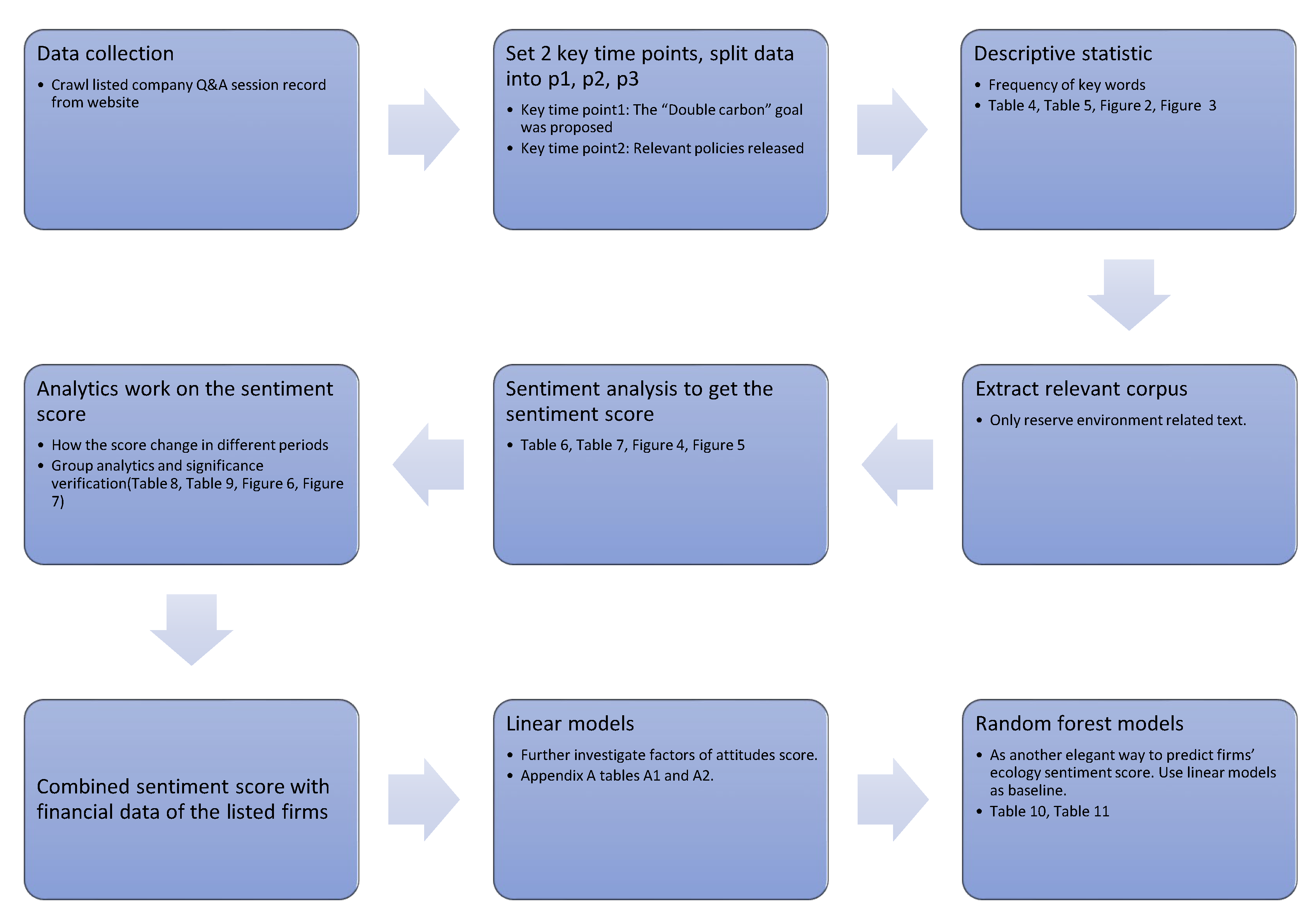

| Variables | Explanation | Source |
|---|---|---|
| company | Name of the invested public firm | East Money’s website |
| com_code | The stock code of the company | |
| date | The date when the Q&A was conducted by investors and the firm | |
| text | The text record of the Q&A | East Money’s website, cleaned by the author; only texts about the environment were preserved |
| weight | The sentiment score calculated from the variable text using sentiment analysis | Calculated by the author |
| period (p1, p2, p3) | The time category of the Q&A record. P1 refers to those from before the “Double Carbon” goal was set. P3 refers to those from after the goal was incorporated into the government’s work report. P2 is the time between p1 and p3. Then, we split p1 into p0 and p1 according to the time of the COVID-19 outbreak in China. When p0 is included, p1 refers to the period between the Wuhan shutdown and when the “Double Carbon” goal was proposed. | The writer set this according to the variable date |
| current_value | of the stock value | Choice dataset from East Money |
| percentage of increase | of the stock value | |
| amount of float | of the stock value | |
| volume | of the stock value | |
| recent trading volume | of the stock value | |
| speed of increment | of the stock value | |
| turnover | of the stock value | |
| volume of transaction | of the stock value | |
| highest value | of the stock value | |
| lowest value | of the stock value | |
| open | of the stock value | |
| close | of the stock value | |
| stock amplitude | of the stock value | |
| quantity relative ratio | of the stock value | |
| price-earnings ratio.TTM. | of the stock value | |
| price-earnings ratio.LYR. | of the stock value | |
| price/book value ratio | of the stock value | |
| market_value | of the stock value | |
| total value | of the stock value | |
| industry | 96 different industries; the industry to which the company belongs | |
| the percentage of float in 60 days | of the stock value | |
| the percentage of float in this year | of the stock value |
| Methods | Findings | |
|---|---|---|
| Descriptive statistics | After the goals were proposed by President Xi and incorporated into government work reports, the frequency of words related to the environment mentioned in investor Q&As increased. | |
| Sentiment analysis (one of the NLP methods) | We obtained the sentiment score for carbon reduction. | |
| Analytics on the sentiment score | Group analytics (Wilcoxon test) |
|
| model1: lm1 |
| |
| model2: lm2 | The sentiment score was significantly influenced by whether a firm was in the technology industry. | |
| model3: rf1 | A non-NLP way to predict firms’ attitudes was provided. | |
| model4: rf2 | ||
| Applied the four models for prediction and estimated the models by using the RMSE (a standard machine learning procedure). | Model3 (rf1) had the best RMSE, which means the lowest error in prediction. | |
| Word | Sentiment Weight |
|---|---|
| sad | −1 |
| very sad | −2 |
| happy | 1 |
| very happy | 2 |
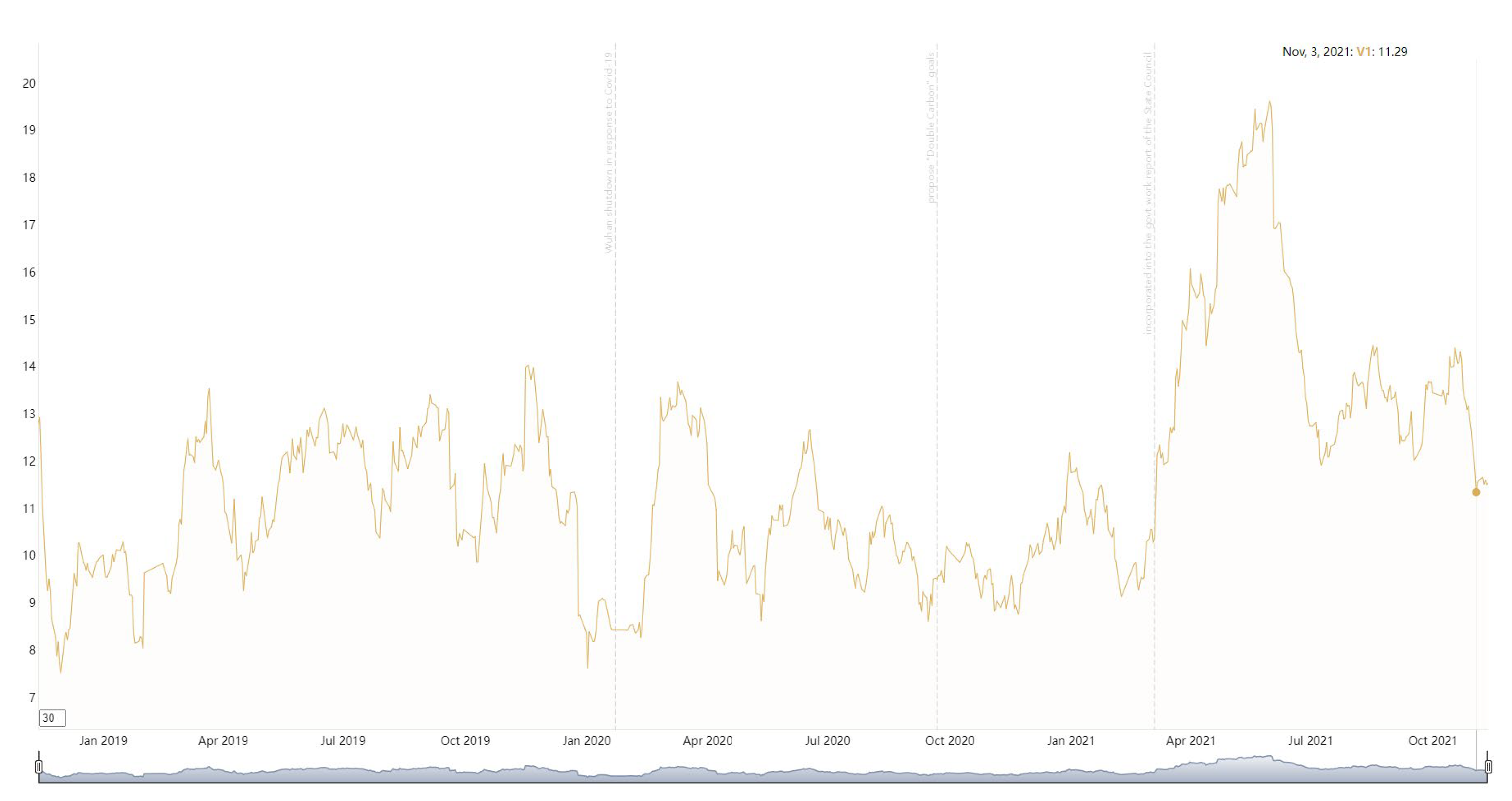
| Date | 13 November 2018 to 22 September 2020 | 22 September 2020 | 22 September 2020 to 5 March 2021 | 5 March 2021 | 5 March 2021 to 12 November 2021 |
| Period | period1 | President Xi proposed China’s “Double Carbon” goal at the United Nations | period2 | The “Double Carbon” goal was written into the State Council’s government work report | period3 |
| Number of data records | 134,731 | 53,309 | 116,282 | ||
| The proportion of the total volume | 44.27% | 17.52% | 38.31% |
| Key words | Period | Frequency | The Proportion of Surveys In Each Period |
|---|---|---|---|
| carbon | period1 | 5379 | 3.9924% |
| period2 | 3673 | 6.89% | |
| period3 | 20,459 | 17.59% | |
| total | 29,511 | ||
| low carbon | period1 | 335 | 0.248% |
| period2 | 638 | 1.197% | |
| period3 | 3678 | 3.16% | |
| total | 4651 | ||
| carbon neutralization | period1 | 8 | 0.005937757% |
| period2 | 699 | 1.3% | |
| period3 | 8702 | 7.48% | |
| total | 9409 | ||
| carbon peak | period1 | 0 | 0 |
| period2 | 182 | 0.34% | |
| period3 | 5239 | 4.5% | |
| total | 5421 | ||
| emission reduction | period1 | 2316 | 1.7% |
| period2 | 1287 | 2.4% | |
| period3 | 5478 | 4.7% | |
| total | 9081 | ||
| energy saving | period1 | 8191 | 6.0795% |
| period2 | 2768 | 5.19% | |
| period3 | 11,430 | 9.829% | |
| total | 22,389 |
| Period | Period1 | Period2 | Period3 |
|---|---|---|---|
| Sentiment weight distribution | Min: −5.000 | Min: −3.00 | Min: −5.00 |
| 1st Qu: 3.000 | 1st Qu: 3.00 | 1st Qu: 3.00 | |
| Median: 6.000 | Median: 7.00 | Median: 8.00 | |
| Mean: 9.155 | Mean: 10.28 | Mean: 12.41 | |
| 3rd Qu: 12.000 | 3rd Qu:15.00 | 3rd Qu: 16.00 | |
| Max: 210.000 | Max: 113.00 | Max: 809.00 | |
| Count | 28,977 | 10,818 | 33,290 |
| Variable | Group1 | Group2 | p | p.Adj | p.Format | p.Signif | Method | |
|---|---|---|---|---|---|---|---|---|
| 1 | avg_senti | p1 | p2 | 0.872064 | 0.87 | 0.87 | ns | Wilcoxon |
| 2 | avg_senti | p1 | p3 | 3.02 × 10⁻¹³ | 9.10 × 10⁻¹³ | 3.00 × 10⁻¹³ | *** | Wilcoxon |
| 3 | avg_senti | p2 | p3 | 6.71 × 10⁻⁹ | 1.30 × 10⁻⁸ | 6.70 × 10⁻⁹ | *** | Wilcoxon |
| Variable | Group1 | Group2 | p | p.Adj | p.Format | p.Signif | Method |
|---|---|---|---|---|---|---|---|
| weight | Internet technology | Internet business | 0.005164 | 1 | 0.00516 | ** | Wilcoxon |
| weight | Internet technology | Chemical fertilizer and pesticide | 1.74 × 10⁻¹⁰ | 5.50 × 10⁻⁷ | 1.70 × 10⁻¹⁰ | *** | |
| weight | Internet technology | New materials | 1.13 × 10⁻²⁸ | 4.40 × 10⁻²⁵ | <2 × 10⁻¹⁶ | *** | |
| weight | Internet technology | Chemical materials | 0.001042 | 1 | 0.00104 | ** | |
| weight | Internet technology | Chemical products | 0.029401 | 1 | 0.0294 | * | |
| weight | Internet technology | chemical/pharmaceutical | 8.32 × 10⁻⁷ | 0.0023 | 8.30 × 10⁻⁷ | *** | |
| A total of 4554 rows were omitted, and 3122 of the 4560 comparison groups had significant differences. The complete results are available at: https://github.com/luyuyuyu/gov_mkt_carbon_nlp/blob/main/by_field.csv (accessed on 3 March 2022). | |||||||
| Term | Estimate | Std.Error | t Value | p.Value | Signif Codes | |
|---|---|---|---|---|---|---|
| 1 | (Intercept) | 101.4944 | 13.512 | 7.511426 | 5.94 × 10⁻¹⁴ | *** |
| 2 | date | −0.00515 | 0.000748 | −6.89541 | 5.43 × 10⁻¹² | *** |
| 3 | current_value | −0.29746 | 0.078357 | −3.79628 | 0.000147 | *** |
| 4 | percentage of increase | 0.732461 | 0.034771 | 21.0652 | 4.35 × 10−98 | *** |
| 5 | amount of float | 0.212833 | 0.102069 | 2.085193 | 0.037057 | * |
| 6 | volume | −1.53 × 10⁻⁸ | 5.04 × 10⁻⁹ | −3.04076 | 0.002361 | ** |
| 7 | recent trading volume | 0.000225 | 4.14 × 10⁻⁵ | 5.447573 | 5.13 × 10⁻⁸ | *** |
| 8 | open | 0.308644 | 0.078796 | 3.91703 | 8.98 × 10⁻⁵ | *** |
| 9 | price–earnings ratio.TTM. | 0.004332 | 0.000467 | 9.268343 | 1.96 × 10⁻²⁰ | *** |
| 10 | total value | −2.44 × 10⁻¹² | 1.36 × 10⁻¹² | −1.7983 | 0.072136 | . |
| 11 | percentage of float in 60 days | −0.03591 | 0.002974 | −12.0773 | 1.55 × 10⁻³³ | *** |
| 12 | percentage of float in this year | 0.005856 | 0.000733 | 7.986153 | 1.42 × 10⁻¹⁵ | *** |
| 13–15 period, compare to p0 | periodp1 | 1.643733 | 0.329841 | 4.983406 | 6.27 × 10⁻⁷ | *** |
| periodp2 | 3.485751 | 0.456308 | 7.639027 | 2.23 × 10⁻¹⁴ | *** | |
| periodp3 | 6.488219 | 0.576821 | 11.24823 | 2.56 × 10⁻²⁹ | *** | |
| 16 | whether_tech0 | 1.149543 | 0.362972 | 3.16703 | 0.001541 | ** |
| 17 | whether_tech1 | 0.365539 | 0.139087 | 2.628136 | 0.008588 | ** |
| The First Step to Add a Variable | ||||
| Start: AIC = 281,527.3 | ||||
| Weight~1 | ||||
| Df | Sum of Sq | RSS | AIC | |
| +industry | 95 | 1,291,719 | 11,364,592 | 276,220 |
| +period | 3 | 130,996 | 12,525,314 | 281,002 |
| +%increase | 1 | 126,483 | 12,529,827 | 281,016 |
| +date | 1 | 84,431 | 12,571,879 | 281,187 |
| +%increase_this_year | 1 | 82,653 | 12,573,657 | 281,195 |
| +amount of float | 1 | 45,136 | 12,611,175 | 281,347 |
| +price-earnings ratio.TTM. | 1 | 34,496 | 12,621,814 | 281,390 |
| +current_value | 1 | 28,360 | 12,627,950 | 281,415 |
| +today | 1 | 26,435 | 12,629,876 | 281,423 |
| +%increase_60days | 1 | 2361 | 12,653,950 | 281,520 |
| +recent_trading_volume | 1 | 2357 | 12,653,954 | 281,520 |
| +volume | 1 | 1855 | 12,654,455 | 281,522 |
| +<none> | 12,656,310 | 281,527 | ||
| +total_value | 1 | 190 | 12,656,120 | 281,529 |
| From the lines above, we found that adding the industry variable to the starting model (weight of ~1) would lead to the best AIC. Thus, the stepwise selection started with a weight of 1 + the field in the next step. | ||||
| Step 2: | ||||
| AIC = 276,219.6 | ||||
| Weight ~ 1 + industry | ||||
| Df | Sum of Sq | RSS | AIC | |
| + period | 3 | 108,204 | 11,256,388 | 275,737 |
| +%increase_this_year | 1 | 64,285 | 11,300,307 | 275,932 |
| + date | 1 | 59,843 | 11,304,748 | 275,952 |
| +amount of float | 1 | 36,591 | 11,328,000 | 276,057 |
| +open | 1 | 5802 | 11,358,790 | 276,196 |
| +current_value | 1 | 5776 | 11,358,816 | 276,196 |
| +amount_of_float | 1 | 2508 | 11,362,083 | 276,210 |
| +total_value | 1 | 1660 | 11,362,931 | 276,214 |
| +volume | 1 | 940 | 11,363,652 | 276,217 |
| +<none> | 11,364,592 | 276,220 | ||
| +%increase_60days | 1 | 298 | 11,364,294 | 276,220 |
| +recent_trading_volume | 1 | 170 | 11,364,422 | 276,221 |
| +price-earnings ratio.TTM. | 1 | 114 | 11,364,477 | 276,221 |
| From the lines above, we found that adding the period would lead to the best AIC. Thus, the stepwise selection started with a weight of ~1 + the field + the period in the next step. | ||||
| Several steps were omitted, and the AIC continued improving until the model became weight ~ industry + period + %increase_this_year + %increase + %increase_60days + date + amount_of_float + current_value + open + total_value + recent_trading_volume + price-earnings ratio.TTM. | ||||
| We can see that in this step, adding the variable “volume” was not better than adding nothing (<none>) according to the AIC. Thus, the stepwise variable selection suggested that we delete the volume variable. | ||||
| Df | Sum of Sq | Rss | AIC | |
| <none> | 11,104,597 | 275,064 | ||
| +volume | 1 | 37.37 | 11,104,560 | 275,066 |
| Model1 (lm1) | Model2 (lm2) | Model3 (rf1) | Model4 (rf2) | |
|---|---|---|---|---|
| RMSE | 13.91493 | 17.63796 | 10.98379 | 12.84664 |
| note | Baseline | Use the whether_tech variable instead of industry in comparison with model 1. | Cannot use the industry variable, since rf models reject factors with too many levels (96 levels in the industry variable). Remove the volume variable in model 1 according to the stepwise selection result. | Add the whether_tech variable in comparison with model 3. |
Publisher’s Note: MDPI stays neutral with regard to jurisdictional claims in published maps and institutional affiliations. |
© 2022 by the authors. Licensee MDPI, Basel, Switzerland. This article is an open access article distributed under the terms and conditions of the Creative Commons Attribution (CC BY) license (https://creativecommons.org/licenses/by/4.0/).
Share and Cite
Li, C.; Li, L.; Zheng, J.; Wang, J.; Yuan, Y.; Lv, Z.; Wei, Y.; Han, Q.; Gao, J.; Liu, W. China’s Public Firms’ Attitudes towards Environmental Protection Based on Sentiment Analysis and Random Forest Models. Sustainability 2022, 14, 5046. https://doi.org/10.3390/su14095046
Li C, Li L, Zheng J, Wang J, Yuan Y, Lv Z, Wei Y, Han Q, Gao J, Liu W. China’s Public Firms’ Attitudes towards Environmental Protection Based on Sentiment Analysis and Random Forest Models. Sustainability. 2022; 14(9):5046. https://doi.org/10.3390/su14095046
Chicago/Turabian StyleLi, Cai, Luyu Li, Jiaqi Zheng, Jizhi Wang, Yi Yuan, Zezhong Lv, Yinghao Wei, Qihang Han, Jiatong Gao, and Wenhao Liu. 2022. "China’s Public Firms’ Attitudes towards Environmental Protection Based on Sentiment Analysis and Random Forest Models" Sustainability 14, no. 9: 5046. https://doi.org/10.3390/su14095046
APA StyleLi, C., Li, L., Zheng, J., Wang, J., Yuan, Y., Lv, Z., Wei, Y., Han, Q., Gao, J., & Liu, W. (2022). China’s Public Firms’ Attitudes towards Environmental Protection Based on Sentiment Analysis and Random Forest Models. Sustainability, 14(9), 5046. https://doi.org/10.3390/su14095046


