
Hydroecology of Argyroneta aquatica’s Habitat in Hantangang River Geopark, South Korea


Abstract
1. Introduction
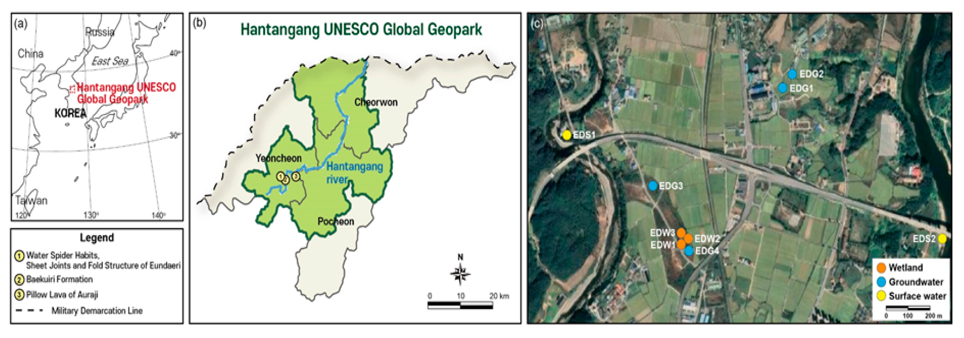
2. Study Area
3. Materials and Methods
3.1. Field Survey and Hydrochemical Analysis Method
3.2. Microbial Analysis Method
3.3. Correlation Analysis Method
4. Results and Discussion
4.1. Hydrochemical Properties
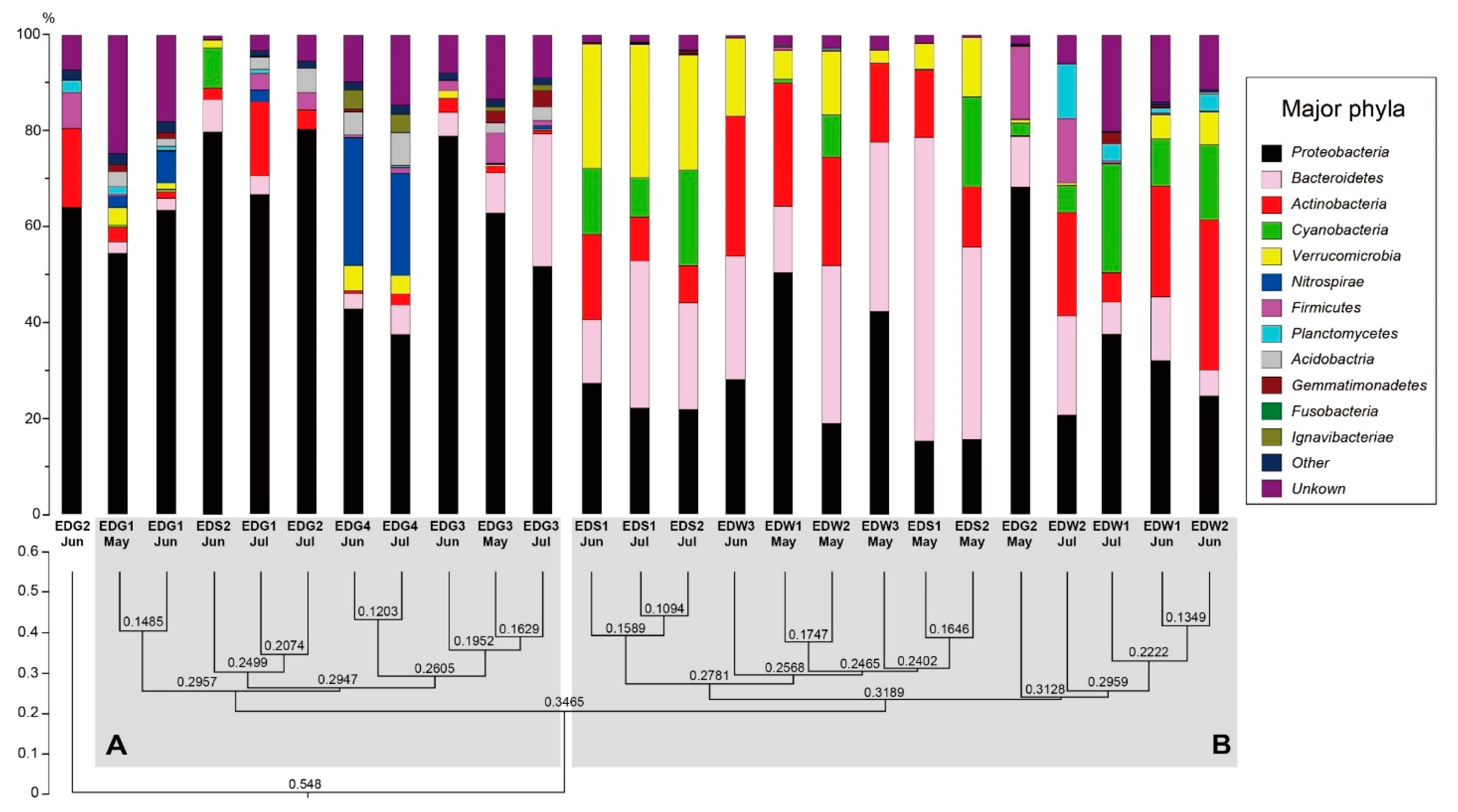
4.2. Phylum-Level Analysis
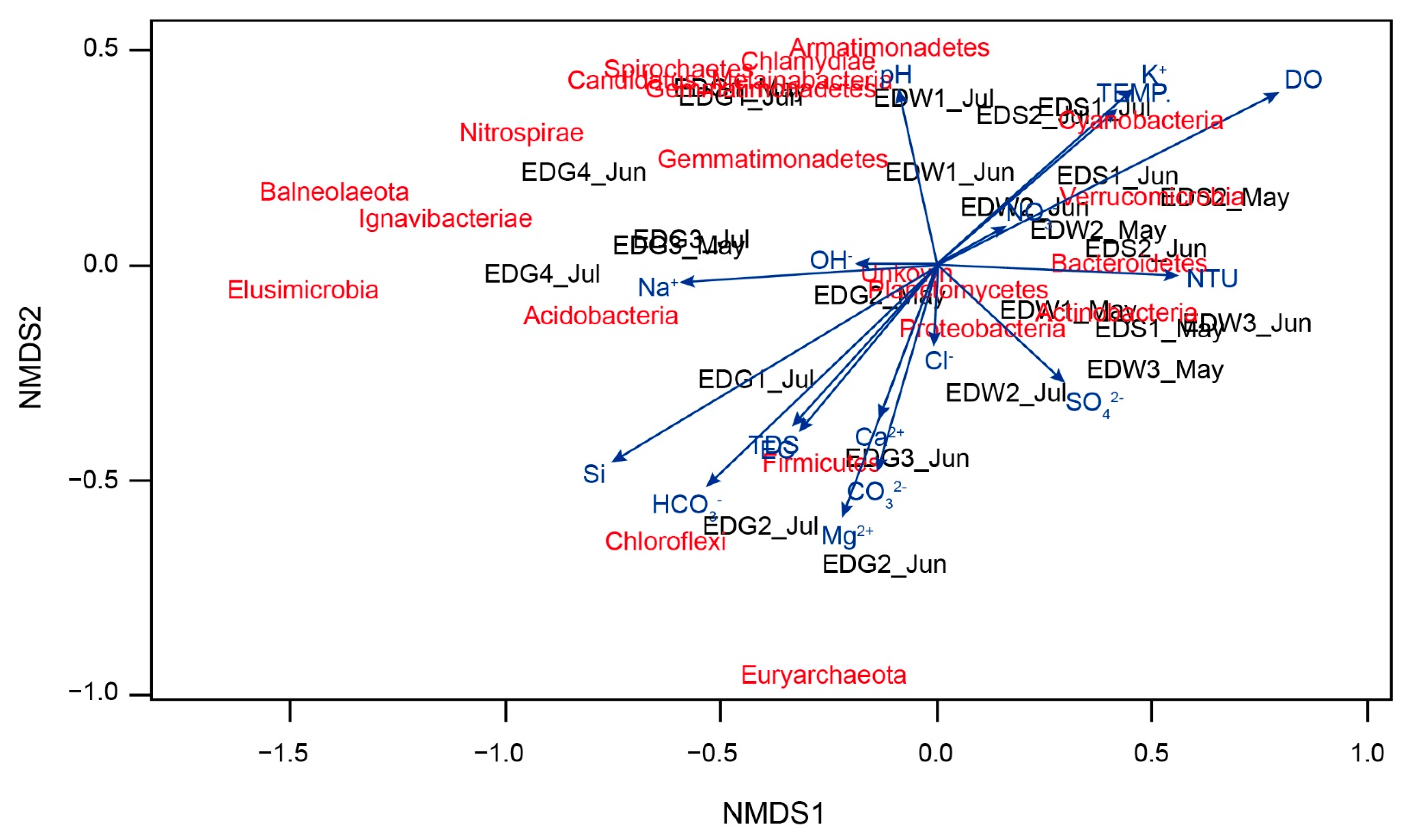
4.3. Non-Metric Multidimensional Scaling (NMDS) and Canonical Correlation Analysis (CCA)
5. Conclusions
Author Contributions
Funding
Institutional Review Board Statement
Informed Consent Statement
Data Availability Statement
Conflicts of Interest
References
- De Bakker, D.; Baetens, K.; Van Nimmen, E.; Gellynck, K.; Mertens, J.; Van Langenhove, L.; Kiekens, P. Description of the structure of different silk threads produced by the water spider Argyroneta aquatica (Clerck, 1757) (Araneae: Cybaeidae). Belg. J. Zool. 2006, 136, 137–143. [Google Scholar]
- Namkung, J.; Kim, S.T.; Lim, H.Y. On a water spider, Argyroneta aquatica (Clerck, 1758) from Korea (Araneae: Argyronetidae). Korean Arachnol. 1996, 12, 111–117. (In Korean) [Google Scholar]
- Bristowe, W.S. The World of Spiders; Collins: London, UK, 1958. [Google Scholar]
- Foelix, R.F. Biology of Spiders; Harvard University Press: Cambridge, UK, 1981; p. 306. [Google Scholar]
- Seyyar, O.; Demir, H. Distribution and habitats of the water spider Argyroneta aquatica (Clerck, 1757) (Araneae, Cybaeidae) in Turkey. Arch. Biol. Sci. 2009, 61, 773–776. [Google Scholar] [CrossRef]
- Seymour, R.S.; Hetz, S.K. The diving bell and the spider: The physical gill of Argyroneta aquatica. J. Exp. Biol. 2011, 214, 2175–2181. [Google Scholar] [CrossRef] [PubMed]
- Masumoto, T.; Masumoto, T.; Yoshida, M.; Nishikawa, Y. Water conditions of the habitat of the water spider Argyroneta aquatica (Araneae; Argyronetidae) in Mizoro pond. Acta Arachnol. 1998, 47, 121–124. [Google Scholar] [CrossRef][Green Version]
- Masumoto, T.; Masumoto, T.; Yoshida, M.; Nishikawa, Y. Time budget of activity in the water spider Argyroneta aquatica (Araneae, Argyronetidae) under rearing conditions. Acta Arachnol. 1998, 47, 125–131. [Google Scholar] [CrossRef][Green Version]
- Mammola, S.; Cavalcante, R.; Isaia, M. Ecological preference of the diving bell spider Argyroneta aquatica in a resurgence of the Po plain (Northern Italy) (Araneae: Cybaeidae). Fragm. Entomol. 2016, 48, 9–16. [Google Scholar] [CrossRef]
- Kim, J.P.; Lim, D.H. Ecological studies of Korean Argyroneta aquatica (Clerck, 1757). Korean Arachnol. 2011, 27, 3–48. (In Korean) [Google Scholar]
- Brignoli, P.M. Ragni d’Italia XXVII. Nuovi dati su Agelenidae, Argyronetidae, Hahniidae, Oxyopidae e Pisauridae, cavernicoli ed epigei (Araneae). Quad. Mus. Speleol. V. Rivera L’Aquila 1977, 2, 3–118. [Google Scholar]
- Dolmen, D. Vannedderkoppen, Argyroneta aquatica Clerck, i Tmndelagsornradet. Fauna 1977, 30, 121–126. [Google Scholar]
- Aakra, K.; Dolmen, D. Distribution and ecology of the water spider, Argyroneta aquatica (Clerck) (Araneae, Cybaeidae), in Norway. Nor. J. Entomol. 2003, 50, 11–16. [Google Scholar]
- Isaia, M.; Pantini, P.; Beikes, S.; Badino, G. Catalogo ragionato dei ragni (Arachnidia, Aranea) del Piemonte e della Lombardia. In Memorie dell’Associazione Naturalistica Piemontese; Paolo Pantini: Torino, Italy, 2007; Volume IX. [Google Scholar]
- Komnenov, M.; Lazarević, P.; Pavićević, D. New records of the water spider Argyroneta aquatica (Clerck, 1757) (Araneae, Cybaeidae) in Serbia. Nat. Montenegrina 2011, 10, 405–414. [Google Scholar]
- IUCN (International Union for the Conservation of Nature and Natural Resource). Integrating Biodiversity Conservation and Sustainable Use; Graham Bennett: Gland, Switzerland; Cambridge, UK, 2004; p. 55. [Google Scholar]
- Bullock, A.; Acreman, M. The role of wetlands in the hydrological cycle. Hydrol. Earth Syst. Sci. 2003, 7, 358–389. [Google Scholar] [CrossRef]
- Shin, Y.H.; Kim, S.H.; Park, S.J. The geochemical roles and properties of mountain wetland in Shinbulsan (Mt.). J. Korean Geomorph. Assoc. 2005, 12, 133–149. (In Korean) [Google Scholar]
- Yang, H.K. The hydrological roles and properties of wangdeungjae wetland in Jirisan. J. Korean Geomorph. Assoc. 2008, 15, 77–85. (In Korean) [Google Scholar]
- Yang, J.H. Geomorphological characteristics of the water spider habitat in Yeoncheon. J. Korean Geomorph. Assoc. 2018, 25, 77–88. (In Korean) [Google Scholar]
- Lim, H.Y. The secret in the pool created by the tank track and habitat discovery of water spider. Nat. Conserv. 1996, 19, 8–11. (In Korean) [Google Scholar]
- Kim, J.P. Coloured Spider of Korea; Academybook: Seoul, Korea, 2002; p. 519. [Google Scholar]
- Pimm, S.L.; Russell, G.J.; Gittleman, J.L.; Brooks, T.M. The future of biodiversity. Science 1995, 269, 347–350. [Google Scholar]
- You, Y.H.; Yi, H.B. Vegetation characteristics, conservation, and ecotourism strategies for water spider (Argyroneta aquatica) in small marsh, Korean Natural Monument. J. Wetl. Res. 2009, 11, 99–106. (In Korean) [Google Scholar]
- Lee, M.B.; Lee, S.; Kim, L.; Cha, M. A Study on the ecological and geomorphological environment of the water spider (Argyroneta aquatica) habitat on the Jeongok Lava Plateau in Yeoncheon, Central Korea. J. Korean Geomorph. Assoc. 2016, 23, 85–99. (In Korean) [Google Scholar]
- Shepard, R.N. Metric structures in ordinal data. J. Math. Psychol. 1996, 3, 287–315. [Google Scholar] [CrossRef]
- Ramette, A. Multivariate analyses in microbial ecology. Fed. Eur. Microbiol. Soc. 2007, 62, 142–160. [Google Scholar] [CrossRef] [PubMed]
- Lee, J.Y.; Hahn, J.S. Characterization of ground-water temperature obtained from the Korean national groundwater monitoring stations: Implications for heat pumps. J. Hydrol. 2006, 329, 514–526. [Google Scholar] [CrossRef]
- Yamagishi, H.; Yoshida, Y.; Fukuhara, H. Methods for Ecology of Aquatic Organisms—Fishes and Bentoth in Fresh Water; Kyoritsu press: Tokyo, Japan, 1976. (In Japanese) [Google Scholar]
- Katsura, K.; Nishikawa, Y. On the habitat environment of the water spider. Atypus 1981, 79, 28–29. (In Japanese) [Google Scholar]
- Piper, A.M. A graphic procedure in the geochemical interpretation of water analyses. Trans. Am. Geophys. Union 1944, 25, 914–928. [Google Scholar] [CrossRef]
- Chadha, D.K. A proposed new diagram for geochemical classification of natural waters and interpretation of chemical data. Hydrogeol. J. 1999, 7, 431–439. [Google Scholar] [CrossRef]
- Guseva, N. The origin of the natural water chemical composition in the permafrost region of the eastern slope of the Polar Urals. Water 2016, 8, 594. [Google Scholar] [CrossRef]
- Giménez-Forcada, E. Dynamic of sea water Interface using hydrochemical facies evolution diagram. Groundwater 2010, 48, 212–216. [Google Scholar] [CrossRef]
- Marchina, C.; Natali, C.; Fazzini, M.; Fusetti, M.; Tassinari, R.; Bianchini, G. Extremely dry and warm conditions in northern Italy during the year 2015: Effects on the Po river water. Rend. Lincei 2017, 28, 281–290. [Google Scholar] [CrossRef]
- Qian, H.; Wu, J.; Li, P. Stable oxygen and hydrogen isotopes as indicators of lake water recharge and evaporation in the lakes of the Yinchuan Plain. Hydrol. Processes 2014, 28, 3554–3562. [Google Scholar] [CrossRef]
- SAHRA. Sustainability of Semi-Arid Hydrology and Riparian Areas; Isotopes: Oxygen, AZ, USA, 2005. [Google Scholar]
- Pang, Z.; Kong, Y.; Li, J.; Tian, J. An isotopic geoindicator in the hydrological cycle. Procedia Earth Planet. Sci. 2017, 17, 534–537. [Google Scholar] [CrossRef]
- Lozupone, C.A.; Hamady, M.; Kelley, S.T.; Knight, R. Quantitative and qualitative diversity measures lead to different insights into factors that structure microbial communities. Appl. Environ. Microbiol. 2007, 73, 1576–1585. [Google Scholar] [CrossRef] [PubMed]
- Ghiorse, W.C.; Wilson, J.T. Microbial ecology of the terrestrial subsurface. Adv. Appl. Microbiol. 1988, 33, 107–172. [Google Scholar]
- Madsen, E.L.; Ghiorse, W.C. Groundwater microbiology: Subsurface ecosystem processes. In Aquatic Microbiology—An Ecological Approach; Ford, T.E., Ed.; Blackwell Scientific Publication: Oxford, UK, 1993; pp. 167–213. [Google Scholar]
- Gold, T. The deep, hot biosphere. Proc. Natl. Acad. Sci. USA 1992, 89, 6045–6049. [Google Scholar] [CrossRef] [PubMed]
- Stevens, T.O.; McKinley, J.P. Lithoautotrophic microbial ecosystems in deep basalt aquifers. Science 1995, 270, 450–454. [Google Scholar] [CrossRef]
- Kotelnikova, S.; Pedersen, K. Evidence for methanogenic Archaea and homoacetogenic Bacteria in deep granitic rock aquifers. FEMS Microbiol. Rev. 1997, 20, 339–349. [Google Scholar] [CrossRef]
- Lithoautotrophy in the subsurface. FEMS Microbiol. Rev. 1997, 20, 327–337. [CrossRef]
- Wolters, N.; Schwartz, W. Untersuchungen über Vorkommen und Verhalten von Mikroorganismen in reinen Grundwässern. Arch. Hydrobiol. 1956, 51, 500–541. [Google Scholar]
- O’Connell, S.P.; Lehman, R.M.; Snoeyenbos-West, O.; Winston, V.D.; Cummings, D.E.; Watwood, M.E.; Colwell, F.S. Detection of Euryarchaeota and Crenarchaeota in an oxic basalt aquifer. FEMS Microbiol. Rev. 2003, 44, 165–173. [Google Scholar]
- Spring, S.; Schulze, R.; Overmann, J.; Schleifer, K.H. Identification and characterization of ecologically significant prokaryotes in the sediment of freshwater lakes: Molecular and cultivation studies. FEMS Microbiol. Rev. 2000, 24, 573–590. [Google Scholar] [CrossRef]
- Liu, L.; Peng, Y.; Zheng, X.H.; Xiao, L.; Yang, L.Y. Vertical structure of bacterial and archaeal communities within the sediment of a eutrophic lake as revealed by culture-independent methods. J. Freshw. Ecol. 2010, 25, 565–573. [Google Scholar] [CrossRef]
- Song, H.; Li, Z.; Du, B.; Wang, G.; Ding, Y. Bacterial communities in sediments of the shallow Lake Dongping in China. J. Appl. Microbiol. 2012, 112, 79–89. [Google Scholar] [CrossRef] [PubMed]
- Qu, J.H.; Yuan, H.L.; Wang, E.T.; Li, C.; Huang, H.Z. Bacterial diversity in sediments of the eutrophic Guanting Reservoir, China, estimated by analyses of 16S rDNA sequence. Biodivers. Conserv. 2008, 17, 1667–1683. [Google Scholar] [CrossRef]
- Roske, K.; Sachse, R.; Scheerer, C.; Roske, I. Microbial diversity and composition of the sediment in the drinking water reservoir Saidenbach (Saxonia, Germany). Syst. Appl. Microbiol. 2012, 35, 35–44. [Google Scholar] [CrossRef]
- Cheng, W.; Zhang, J.X.; Wang, Z.; Wang, M.; Xie, S.G. Bacterial communities in sediments of a drinking water reservoir. Ann. Microbiol. 2013, 64, 875–878. [Google Scholar] [CrossRef]
- Ehrich, S.; Behrens, D.; Ludwig, W.; Bock, E. A new obligately chemolithoautotrophic, nitrite-oxidizing bacterium, nitrospira moscoviensis sp. nov. and its phylogenetic relationship. Arch. Microbiol. 1995, 164, 16–23. [Google Scholar] [CrossRef]
- Li, J.; Chen, Q.; Li, Q.; Zhao, C.; Feng, Y. Influence of plants and environmental variables on the diversity of soil microbial communities in the Yellow River Delta Wetland, China. Chemosphere 2021, 274, 129967. [Google Scholar] [CrossRef]
- Ghai, R.; Rodriguez-Valera, F.; McMahon, K.D.; Toyama, D.; Rinke, R.; Cristina Souza de Oliveira, T.; Wagner Garcia, J.; Pellon de Miranda, F.; Henrique-Silva, F. Metagenomics of the water column in the pristine upper course of the Amazon river. PLoS ONE 2011, 6, e23785. [Google Scholar] [CrossRef]
- Servin, J.A.; Herbold, C.W.; Skophammer, R.G.; Lake, J.A. Evidence excluding the root of the tree of life from the actinobacteria. Mol. Biol. Evol. 2008, 25, 1–4. [Google Scholar] [CrossRef]
- Zhu, X.; Wang, L.; Zhang, X.; He, M.; Wang, D.; Ren, Y.; Yao, H.; Ngegla, J.; Pan, H. Effects of different types of anthropogenic disturbances and natural wetlands on water quality and microbial communities in a typical black-odor river. Ecol. Indic. 2022, 136, 108613. [Google Scholar] [CrossRef]
- He, S.; Stevens, S.L.R.; Chan, L.K.; Bertilsson, S.; Rio, T.; Tringe, S.; Malmstrom, R.; McMahon, K. Ecophysiology of freshwater Verrucomicrobia inferred from metagenome-assembled genomes. mSphere 2017, 2, e00277-17. [Google Scholar] [CrossRef] [PubMed]
- Zwart, G.; van Hannen, E.J.; Kamst-van Agterveld, M.P.; Van der Gucht, K.; Lindström, E.S.; Van Wichelen, J.; Lauridsen, T.; Crump, B.C.; Han, S.K.; Declerck, S. Rapid screening for freshwater bacterial groups by using reverse line blot hybridization. Appl. Environ. Microbiol. 2003, 69, 5875–5883. [Google Scholar] [CrossRef] [PubMed]
- Newton, R.J.; Jones, S.E.; Eiler, A.; McMahon, K.D.; Bertilsson, S. A guide to the natural history of freshwater lake bacteria. Microbiol. Mol. Biol. Rev. 2011, 75, 14–49. [Google Scholar] [CrossRef] [PubMed]
- Eiler, A.; Bertilsson, S. Composition of freshwater bacterial communities associated with cyanobacterial blooms in four Swedish lakes. Environ. Microbiol. 2004, 6, 1228–1243. [Google Scholar] [CrossRef] [PubMed]
- Parveen, B.; Mary, I.; Vellet, A.; Ravet, V.; Debroas, D. Temporal dynamics and phylogenetic diversity of free-living and particle-associated Verrucomicrobia communities in relation to environmental variables in a mesotrophic lake. FEMS Microbiol. Ecol. 2013, 83, 189–201. [Google Scholar] [CrossRef] [PubMed]
- Arnds, J.; Knittel, K.; Buck, U.; Winkel, M.; Amann, R. Development of a 16S rRNA-targeted probe set for Verrucomicrobia and its application for fluorescence in situ hybridization in a humic lake. Syst. Appl. Microbiol. 2010, 33, 139–148. [Google Scholar] [CrossRef]
- Madigan, M.T.; Martinko, J.M.; Buckley, D.H.; Bender, K.S.; Stahl, D. Brock Biology of Microorganisms, 14th ed.; Pearson: London, UK, 2015. [Google Scholar]
- Deep, P.; Bhattacharyya, S.; Nayak, B. Cyanobacteria in wetlands of the industrialized Sambalpur District of India. Aquat. Biosyst. 2013, 9, 14. [Google Scholar] [CrossRef]
- Le Maitre, R.W.; Bateman, P.; Dudek, A.; Keller, J.; Lameyre Le Bas, M.J.; Sabine, P.A.; Schmid, R.; Sorensen, H.; Streckeisen, A.; Woolley, A.R.; et al. A Classification of Igneous Rocks and Glossary of Terms; Blackwell: Oxford, UK, 1989. [Google Scholar]
- Parker, C.W.; Auler, A.S.; Barton, M.D.; Sasowsky, I.D.; Senko, J.M.; Barton, H.A. Fe(III) reducing microorganisms from iron ore caves demonstrate fermentative Fe(III) reduction and promote cave formation. Geomicrobiol. J. 2017, 35, 311–322. [Google Scholar] [CrossRef]
- Baker, P.; Bellifemine, D. Environmental influences on akinete germination of Anabaena circinalis and implications for management of cyanobacterial blooms. Hydrobiologia 2000, 47, 65–73. [Google Scholar] [CrossRef]
- De Figueiredo, D.R.; Pereira, M.J.; Moura, A.; Silva, L.; Barrios, S.; Fonseca, F.; Henriques, I.; Correia, A. Bacterial community composition over a dry winter in meso- and eutrophic Portuguese water bodies. FEMS Microbiol. Ecol. 2007, 59, 638–650. [Google Scholar] [CrossRef]
- Heinzel, E.; Janneck, E.; Glombitza, F.; Schlömann, M.; Seifert, J. Population dynamics of iron-oxidizing communities in pilot plants for the treatment of acid mine waters. Environ. Sci. Technol. 2009, 43, 6138–6144. [Google Scholar] [CrossRef] [PubMed]
- Lipko, I.; Belykh, O. Environmental features of freshwater planktonic actinobacteria. Contemp. Probl. Ecol. 2021, 14, 158–170. [Google Scholar] [CrossRef]
- Xue, Y.; Shen, J.; Chen, Z.; Ma, J. Isolation and cultivation of actinomycetes causing T&Os and detection of its metabolized T&O compounds. J. Harbin Inst. Technol. 2008, 40, 563–567. [Google Scholar]
- Zhang, H.; Ma, M.; Huang, T.; Miao, Y.; Li, H.; Liu, K.; Yang, W.; Ma, B. Spatial and temporal dynamics of actinobacteria in drinking water reservoirs: Novel insights into abundance, community structure, and co-existence model. Sci. Total Environ. 2022, 814, 152804. [Google Scholar] [CrossRef] [PubMed]


| Country | Average Temperature (°C) | Average Precipitation (mm) |
|---|---|---|
| United Kingdom | 9.3 | 1466.4 |
| Ireland | 10.0 | 1306.6 |
| Netherland | 10.8 | 913.5 |
| Germany | 10.0 | 688.9 |
| Norway | 7.0 | 8.7 |
| Japan | 16.5 | 1658.9 |
| Australia | 0.9 | 473.0 |
| Parameter | Temperature (°C) | pH | EC (μS/cm) | DO (mg/L) | ORP (mV) | Turbidity (NTU) | |
|---|---|---|---|---|---|---|---|
| EDW1 | Max | 37.7 | 9.1 | 93.3 | 9.5 | 111.2 | 40.2 |
| Min | 19.2 | 7.4 | 86.3 | 7.4 | 21.4 | 26.9 | |
| Mean | 29.0 | 8.3 | 88.9 | 8.7 | 53.2 | 31.4 | |
| SD * | 9.3 | 0.8 | 3.8 | 1.1 | 27.6 | 7.6 | |
| CV ** | 0.3 | 0.1 | 0.0 | 0.1 | 0.5 | 0.2 | |
| EDW2 | Max | 36.9 | 9.2 | 77.4 | 9.1 | 72.1 | 21.4 |
| Min | 19.9 | 7.2 | 66.5 | 7.7 | 24.2 | 17.2 | |
| Mean | 28.8 | 8.4 | 73.6 | 8.6 | 47.7 | 19.0 | |
| SD * | 8.5 | 1.1 | 6.2 | 0.8 | 24.0 | 2.2 | |
| CV ** | 0.3 | 0.1 | 0.1 | 0.1 | 0.5 | 0.1 | |
| EDW3 | Max | 30.2 | 7.9 | 56.6 | 11.0 | 85.9 | 48.2 |
| Min | 20.6 | 7.6 | 44.6 | 8.7 | 58.7 | 27.5 | |
| Mean | 25.4 | 7.7 | 50.6 | 9.8 | 72.3 | 37.9 | |
| SD * | 6.8 | 0.2 | 8.5 | 1.6 | 19.2 | 14.6 | |
| CV ** | 0.3 | 0.0 | 0.2 | 0.2 | 0.3 | 0.4 | |
| EDS1 | Max | 30.7 | 8.6 | 281.5 | 9.9 | 70.5 | 10.0 |
| Min | 16.7 | 7.7 | 212.8 | 8.3 | 45.1 | 6.6 | |
| Mean | 25.2 | 8.3 | 247.7 | 9.1 | 59.4 | 8.3 | |
| SD * | 7.4 | 0.5 | 34.4 | 0.8 | 13.0 | 1.7 | |
| CV ** | 0.3 | 0.1 | 0.1 | 0.1 | 0.2 | 0.2 | |
| EDS2 | Max | 31.8 | 8.6 | 388.9 | 9.5 | 90.6 | 15.0 |
| Min | 17.3 | 7.7 | 242.0 | 7.1 | 54.8 | 9.4 | |
| Mean | 25.0 | 8.1 | 328.6 | 8.5 | 73.6 | 11.7 | |
| SD * | 7.3 | 0.5 | 76.9 | 1.2 | 18.0 | 2.9 | |
| CV ** | 0.3 | 0.1 | 0.2 | 0.1 | 0.2 | 0.3 | |
| EDG1 | Max | 19.1 | 7.5 | 284.7 | 7.5 | 105.7 | 16.1 |
| Min | 14.2 | 6.6 | 257.5 | 6.6 | 89.0 | 0.4 | |
| Mean | 16.3 | 7.1 | 269.7 | 7.0 | 98.2 | 6.3 | |
| SD * | 2.5 | 0.5 | 13.8 | 0.5 | 8.5 | 8.6 | |
| CV ** | 0.2 | 0.1 | 0.1 | 0.1 | 0.1 | 1.4 | |
| EDG2 | Max | 20.1 | 6.7 | 550.0 | 5.0 | 112.8 | 21.9 |
| Min | 14.1 | 6.6 | 525.0 | 4.5 | 76.8 | 9.0 | |
| Mean | 17.0 | 6.7 | 540.0 | 4.8 | 98.9 | 14.4 | |
| SD * | 3.0 | 0.1 | 13.2 | 0.3 | 19.4 | 6.6 | |
| CV ** | 0.2 | 0.0 | 0.0 | 0.1 | 0.2 | 0.5 | |
| EDG3 | Max | 19.1 | 8.1 | 245.6 | 3.5 | 71.1 | 0.7 |
| Min | 14.4 | 8.0 | 235.4 | 2.8 | −3.3 | 0.3 | |
| Mean | 16.8 | 8.0 | 240.3 | 3.1 | 27.3 | 0.5 | |
| SD * | 2.4 | 0.1 | 5.1 | 0.4 | 38.9 | 0.2 | |
| CV ** | 0.1 | 0.0 | 0.0 | 0.1 | 1.4 | 0.4 | |
| EDG4 | Max | 18.2 | 9.7 | 284.1 | 3.6 | 1.4 | 1.0 |
| Min | 16.6 | 9.7 | 280.3 | 2.1 | −0.3 | 0.5 | |
| Mean | 17.4 | 9.7 | 282.2 | 2.8 | 0.6 | 0.8 | |
| SD * | 1.1 | 0.0 | 2.7 | 1.0 | 1.2 | 0.3 | |
| CV ** | 0.1 | 0.0 | 0.0 | 0.4 | 2.2 | 0.4 | |
| Sample | NO3− (mg/L) | Sample | NO3− (mg/L) | Sample | NO3− (mg/L) |
|---|---|---|---|---|---|
| EDW1 May | non-detection | EDW1 June | non-detection | EDW1 July | non-detection |
| EDW2 May | non-detection | EDW2 June | non-detection | EDW2 July | non-detection |
| EDW3 May | non-detection | EDW3 June | non-detection | ||
| EDS1 May | 17.74 | EDS1 June | 9.42 | EDS1 July | 6.99 |
| EDS2 May | 15.38 | EDS2 June | 10.86 | EDS2 July | 10.29 |
| EDG1 May | 12.09 | EDG1 June | 12.03 | EDG1 July | 11.87 |
| EDG2 May | 7.3 | EDG2 June | 9.19 | EDG2 July | 8.57 |
| EDG3 May | 0.87 | EDG3 June | 1.19 | EDG3 July | non-detection |
| EDG4 June | 0.72 | EDG4 July | 0.63 |
| Sample | OTUs | Chao1 | Shannon | Inverse Simpson | Good’s Coverage of Library (%) |
|---|---|---|---|---|---|
| EDW1 May | 158 | 181.21 | 6.03 | 0.97 | 99.05 |
| EDW2 May | 139 | 155.15 | 5.80 | 0.97 | 99.23 |
| EDW3 May | 137 | 147.12 | 5.48 | 0.96 | 99.16 |
| EDS1 May | 143 | 158.00 | 5.34 | 0.92 | 99.09 |
| EDS2 May | 117 | 119.40 | 5.37 | 0.95 | 99.67 |
| EDG1 May | 260 | 278.50 | 6.55 | 0.97 | 98.61 |
| EDG2 May | 111 | 118.58 | 4.63 | 0.86 | 99.49 |
| EDG3 May | 111 | 111.14 | 5.15 | 0.94 | 99.89 |
| EDW1 June | 310 | 384.38 | 6.63 | 0.97 | 96.90 |
| EDW2 June | 152 | 159.16 | 5.68 | 0.95 | 99.38 |
| EDW3 June | 58 | 62.50 | 3.50 | 0.85 | 99.67 |
| EDS1 June | 151 | 153.37 | 5.85 | 0.95 | 99.63 |
| EDS2 June | 108 | 110.15 | 5.28 | 0.94 | 99.70 |
| EDG1 June | 186 | 207.14 | 5.86 | 0.96 | 98.87 |
| EDG2 June | 54 | 55.00 | 4.62 | 0.95 | 99.89 |
| EDG3 June | 150 | 161.00 | 4.95 | 0.90 | 99.2 |
| EDG4 June | 168 | 190.96 | 4.74 | 0.88 | 98.8 |
| EDW1 July | 146 | 154.00 | 5.91 | 0.96 | 99.38 |
| EDW2 July | 196 | 207.32 | 6.17 | 0.97 | 99.01 |
| EDS1 July | 236 | 283.28 | 6.04 | 0.95 | 97.74 |
| EDS2 July | 275 | 330.86 | 6.32 | 0.95 | 97.49 |
| EDG1 July | 204 | 205.49 | 6.60 | 0.98 | 99.6 |
| EDG2 July | 54 | 54.00 | 4.63 | 0.94 | 100 |
| EDG3 July | 229 | 278.52 | 5.66 | 0.95 | 97.52 |
| EDG4 July | 308 | 364.84 | 6.44 | 0.96 | 97.05 |
| Vectors | NMDS1 | NMDS1 | r2 | Pr (>r) |
|---|---|---|---|---|
| Temperature | 0.75617 | 0.65437 | 0.2559 | 0.046 * |
| pH | −0.20040 | 0.97971 | 0.1408 | 0.187 |
| EC | −0.63930 | −0.76896 | 0.2134 | 0.063 |
| DO | 0.89139 | 0.45323 | 0.6665 | 0.001 *** |
| TDS | −0.66705 | −0.74502 | 0.2058 | 0.070 |
| NTU | 0.99896 | −0.04559 | 0.2723 | 0.030 * |
| Ca2+ | −0.35112 | −0.93633 | 0.1172 | 0.236 |
| K+ | 0.74672 | 0.66514 | 0.3178 | 0.012 * |
| Mg2+ | −0.35251 | −0.93581 | 0.3222 | 0.008 ** |
| Na+ | −0.99727 | −0.07383 | 0.2950 | 0.023 * |
| Si | −0.85498 | −0.51866 | 0.6455 | 0.001 *** |
| Cl− | −0.01334 | −0.99991 | 0.0258 | 0.756 |
| NO3− | 0.87322 | 0.48732 | 0.0269 | 0.747 |
| SO42− | 0.74050 | −0.67206 | 0.1351 | 0.193 |
| HCO3− | −0.72161 | −0.69230 | 0.4545 | 0.003 ** |
| CO32− | −0.27701 | −0.96087 | 0.2095 | 0.049 * |
| OH− | −0.99994 | −0.01062 | 0.0282 | 0.792 |
| Vectors | Df | ChiSquare | F | Pr (>F) |
|---|---|---|---|---|
| Temperature | 1 | 0.132 | 7.32 | 0.001 *** |
| pH | 1 | 0.145 | 8.02 | 0.001 *** |
| EC | 1 | 0.075 | 4.17 | 0.005 ** |
| DO | 1 | 0.095 | 5.28 | 0.001 *** |
| TDS | 1 | 0.009 | 0.49 | 0.834 |
| NTU | 1 | 0.027 | 1.48 | 0.199 |
| Ca2+ | 1 | 0.022 | 1.21 | 0.318 |
| K+ | 1 | 0.087 | 4.83 | 0.004 ** |
| Mg2+ | 1 | 0.065 | 3.63 | 0.004 ** |
| Na+ | 1 | 0.034 | 1.87 | 0.115 |
| Si | 1 | 0.026 | 1.43 | 0.208 |
| Cl− | 1 | 0.046 | 2.53 | 0.037 * |
| NO3− | 1 | 0.018 | 1.02 | 0.403 |
| SO42− | 1 | 0.029 | 1.62 | 0.168 |
| HCO3− | 1 | 0.017 | 0.96 | 0.451 |
| CO32− | 1 | 0.020 | 1.08 | 0.399 |
| OH− | 1 | 0.025 | 1.41 | 0.243 |
| Residual | 7 | 0.126 |
Publisher’s Note: MDPI stays neutral with regard to jurisdictional claims in published maps and institutional affiliations. |
© 2022 by the authors. Licensee MDPI, Basel, Switzerland. This article is an open access article distributed under the terms and conditions of the Creative Commons Attribution (CC BY) license (https://creativecommons.org/licenses/by/4.0/).
Share and Cite
Moon, J.; Kim, H.; Ryu, H.-S. Hydroecology of Argyroneta aquatica’s Habitat in Hantangang River Geopark, South Korea. Sustainability 2022, 14, 4988. https://doi.org/10.3390/su14094988
Moon J, Kim H, Ryu H-S. Hydroecology of Argyroneta aquatica’s Habitat in Hantangang River Geopark, South Korea. Sustainability. 2022; 14(9):4988. https://doi.org/10.3390/su14094988
Chicago/Turabian StyleMoon, Jinah, Heejung Kim, and Han-Sun Ryu. 2022. "Hydroecology of Argyroneta aquatica’s Habitat in Hantangang River Geopark, South Korea" Sustainability 14, no. 9: 4988. https://doi.org/10.3390/su14094988
APA StyleMoon, J., Kim, H., & Ryu, H.-S. (2022). Hydroecology of Argyroneta aquatica’s Habitat in Hantangang River Geopark, South Korea. Sustainability, 14(9), 4988. https://doi.org/10.3390/su14094988