Article

Multi-Asset Defect Hotspot Prediction for Highway Maintenance Management: A Risk-Based Machine Learning Approach

William State Lee College of Engineering, University of North Carolina at Charlotte, Charlotte, NC 28223, USA
*
Author to whom correspondence should be addressed.
Sustainability 2022, 14(9), 4979; https://doi.org/10.3390/su14094979
Submission received: 8 March 2022 / Revised: 13 April 2022 / Accepted: 19 April 2022 / Published: 21 April 2022

Abstract

:
Transportation agencies constantly strive to tackle the challenge of limited budgets and continuously deteriorating highway infrastructure. They look for optimal solutions to make intelligent maintenance and repair investments. Condition prediction of highway assets and, in turn, prediction of their maintenance needs are key elements of effective maintenance optimization and prioritization. This paper proposes a novel risk-based framework that expands the potential of available data by considering the probabilistic susceptibility of assets in the prediction process. It combines a risk score generator with machine learning to forecast the hotspots of multiple defects while considering the interrelations between defects. With this, we developed a scalable algorithm, Multi-asset Defect Hotspot Predictor (MDHP), and then demonstrated its performance in a real-world case. In the case study, MDHP predicted the hotspots of three defects on paved ditches, considering the interrelation between paved ditches and five nearby assets. The results demonstrate an acceptable accuracy in predicting hotspots while highlighting the interrelation between adjacent assets and their contribution to future defects. Overall, this study offers a scalable approach with contribution in data-driven multi-asset maintenance planning with potential benefits to a broader range of linear infrastructures such as sewers, water networks, and railroads.

1. Introduction

Most U.S. interstate highways, as in most developed countries, have passed or will exceed their design life in the next 20 years and require restorations and preservations [1]. Hence, transportation agencies attempt to maintain roadways in a good state of repair by making significant investments in preserving highway assets. With this, transportation agencies are constantly striving to tackle the challenge of constrained budgets and continuously degrading assets by looking for optimal solutions that make their investments effective and efficient [2,3,4,5]. For this purpose, predictive analytics coupled with advanced sensing technologies and extensive data collection can be leveraged in efficient decision making, maintenance prioritizing, and life-cycle planning [6,7]. However, given the length of roadways, intensifying data collection across all asset classes is expensive and far-fetched for most agencies. Also, the current practice of data collection in transportation agencies is mainly centered around high capital assets (i.e., pavement and bridge). As a result, other assets, especially roadside asset types such as drainage systems, slopes, and signs, have gained less attention leading to the lack of enough data for developing accurate prediction models [8]. Therefore, there is a need to augment the potential of the currently available data to maximize the accuracy of prediction models. In addition, systematically identifying the best algorithm with the best performance in the highway maintenance context facilitates developing more accurate prediction models, and therefore, better maintenance management.
Several studies have contributed to the literature by developing deterioration models. However, in our review, we identified three major gaps in predictive algorithms, which are listed below:
  • Marginal Attention to the Interrelations Between Asset Classes: Due to the mutual impacts of nearby assets and similar environmental conditions in their proximity, there is a potential correlation between the condition of neighboring asset classes. A few research studies have investigated such correlations [9,10,11]. However, the majority of the developed deterioration models in the literature did not take into consideration such interrelations and investigated the condition of each asset independent from its neighbors [12,13,14,15,16,17,18]. For example, Abaza et al. [12] forecasted pavement condition only based on historical condition data of pavements. As another example, Immaneni et al. [16] developed prediction models for traffic signs only based on age and retroreflectivity data of the signs.
  • Shortcomings of Predictive Frameworks in Dealing with Limited Inspection Data: Random inspection of roadways is the current practice of most transportation agencies that restrict the number of segments with adequate historical condition data of road assets. This usually results in discontinuous records of historical conditions on most road segments during all years of inspection. To overcome this limitation, most of the previous studies used the idea of grouping segments with similar deterioration characteristics (family groups) and estimating the average degradation of each group by utilizing a family deterioration model. For example, Mills et al. [19] developed family pavement performance models to help the Delaware DOT in managing road pavements. In another study, Saha et al. [20] used the family group idea to come up with pavement distress deterioration models. However, several challenges come with this approach. Firstly, the condition of specific segments in a family might be different from the average condition of the family. This is mainly attributed to the local variation of contributors to the degradation of assets such as traffic, weather, and maintenance [21]. Secondly, since the number of families highly impacts the accuracy of family deterioration models finding the optimal number of families is still challenging [22].
  • Subjective Expert-based Selection of Contributing Factors to Assets Degradation: Several factors impact the condition of roadway assets and could be considered as the contributing factors to their deterioration. For example, the role of material, traffic loading, weather condition, and historical maintenance on the degradation patterns of multiple assets was highlighted in several studies [12,23,24,25,26,27,28,29,30]. For example, the study performed by Anyala et al. [23] highlighted the impacts of the thickness of flexible pavements and the binder type as two main factors on the resistance of the pavement layer against degradation. As another example, Bannour et al. [24] addressed the role of different ranges of pavements structural composition, environment, moisture and traffic conditions on the deterioration of pavements. However, most studies developed deterioration models when a selected number of contributing factors were considered based on experts’ judgment. In addition, historical maintenance activities, as a major factor that improves the condition of highway assets, have received marginal attention in building previous prediction models [31].
To overcome the deficiencies of previous models, we propose a risk-based prediction method, Multi-asset Defect Hotspot Predictor (MDHP). The proposed framework combines a risk score generator and a Machine Learning (ML) algorithm to predict the hotspots of multiple defects in a given roadway. For this purpose, the objectives of this study are (1) augmenting the limited extent of available inspection data by using density estimation of defects and developing a risk-based prediction approach, (2) creating a predictive scheme that considers the correlations between nearby assets in addition to a wide range of other factors with the potential contribution to the degradation, (3) creating a data-driven approach for finding and selecting major contributing factors in contrast to subjective selections. To achieve these objectives robustly and reliably, we selected and compared multiple ML algorithms ranging from linear to nonlinear categories to offer a procedure for finding the best fit for the problem. The model’s outcome is a set of risk maps that present the predicted hotspots of each defect for the considered asset types in a given road. In this context, hotspots refer to parts of roadways that witness a higher defect density. Overall, the MDHP framework contributes to the body of knowledge by:
  • Maximizing the potential of available data in building prediction models by combining machine learning and risk score generator, offering transportation agencies a practical predictive maintenance planning
  • Incorporating the interrelations of defects in multiple nearby assets into a defect prediction method
  • Developing a data-driven approach to identify and quantify the most significant contributors to the degradation of multiple assets among a wide range of potential candidates
  • Creating a scalable learning-based algorithm to improve maintenance planning for a combination of assets by forecasting the occurrence probability of various defects on multiple asset types
In the following sections, we will first explore the related works. The, we will go through the details of the proposed MDPH method, followed by a case study to present the results of the framework’s performance when applied to a real-world problem. Finally, the key finding of the study will be discussed and concluded.

2. Related Works

2.1. Machine Learning in Transportation Asset Management

Machine learning (ML) techniques have provided scientists and researchers in different fields with opportunities in problem-solving and decision-making that ended up addressing the limitations of traditional statistical modeling. Subjective assumptions and simplifications have been some of the limitations of deterministic and probabilistic approaches utilized in highway asset management [31]. Moreover, only statistical models such as linear regression were traditionally used in developing performance prediction models [32,33]. However, due to the large number of contributors and the complex dynamic of defects in highway assets, such models seemed to be less effective in capturing the underlying behavior of defects [34]. These shortcomings sometimes have caused inconsistencies between the predictions and the actual recorded data, ultimately resulting in inaccurate outcomes. Therefore, in recent years, highway asset management researchers and practitioners have transitioned from traditional approaches to ML-based techniques. For example, Swargam [35] leveraged Artificial Neural Network (ANN) to forecast the performance of traffic signs retro-reflectivity. In another study, Haider et al. [36] investigated the Florida Department of Transportation’s pavement condition data to predict cracking on flexible pavements using ANN. Furthermore, Karwa et al. [37] proposed and explored the application of ANN in projecting retro-reflectivity of pavement markings. Karlaftis et al. [38] provided an ML-based prediction model leveraging a genetically optimized network to forecast the probability of alligator crack initiation on pavements. Finally, Marcelino et al. [39] used an ML approach in investigating pavement performance in the future in pavement management systems (PMS).
In summary, most research studies cited the potential of ML algorithms in increasing the overall quality of prediction modeling in highway asset management [38,40]. In addition, the literature highlights that using ML-based models usually results in more scalable and extensible prediction models compared to deterministic and probabilistic approaches [41,42]. However, the majority of previous research studies mainly focused on the traditional ANN approach and did not invest in other ML techniques with proven performance, such as tree-based models (e.g., decision trees, random forests, and adaptive boosting). In addition, we identified that pavements, as a capital asset class, gained the majority of attention when developing machine learning-based prediction models, and other asset types, especially roadside assets, were limitedly considered. Therefore, it seems that traditional deterministic and probabilistic approaches are still the prevailing techniques for predicting the condition of roadside asset types, and there is room for further investment in ML-based modeling of such assets.

2.2. Risk-Based Predictive Modelling

Risk-based prediction models are specific predictions that provide information on the probability of undesired events. Such models can also be utilized in estimating risks throughout roadways. This mainly stems from the fact that risk is usually defined as the probability of undesired events multiplied by their impacts [43,44]. By utilizing such information, researchers and practitioners have acknowledged the potential of risk maps as an efficient tool in identifying and visualizing the spatial distribution of the risk of undesirable events in different fields. For instance, several studies used the recorded data of fire events in forests to visualize high-risk zones in terms of their susceptibility to wildfire [45,46,47]. As another example, Gaull et al. [48] used historical data of recorded earthquake contents to highlight areas more prone to witness higher seismic impacts. Some researchers also used a similar approach in analyzing road traffic accidents by identifying hotspots of probable accidents [49,50,51]
Several studies also attempted to develop predictive risk-based models and risk maps for roadway infrastructure. For example, Hunt [52] developed a framework for preparing slope failure risk maps that present the level of risk of slope failures in a roadway system. Sohn [53] evaluated the significance of the links in a highway network under flood damage risks. In another study, Wright et al. [54] assessed the potential risks of river flooding due to climate change on bridges. Moreover, Anderson et al. [55] developed a methodology to evaluate the risk and vulnerability of bridges under climate change and extreme weather. Finally, Lu [56] developed a quantitative pavement flooding risk assessment utilizing flood hazard analysis and vulnerability evaluations.
We conclude that previous studies mainly focused on risk prediction and risk-map generation in highway systems under natural hazards and environmental events such as flooding and landslides. However, considering the fact that defects are a major problem in highway infrastructure that negatively impact the condition of assets, there is room for leveraging risk-based forecasting of defects in highway assets. Such information could potentially further strengthen the quality and accuracy of risk-based decision-making in Transportation Asset Management (TAM) programs, with the ability to improve risk management, inspection prioritization, and maintenance optimization decisions.
In this paper, we propose a framework, MDHP, that systematically combines a risk generator and an ML-based predictor to forecast risk-based hotspots of different defects on different types of highway assets while incorporating the inter-relationships of nearby assets. In the next section, we will explain our methodology in detail.

3. Methodology

The devised methodology, as shown in Figure 1, includes seven steps. In step 1, the data of contributing factors will be first collected. Then, in step 2, raw weather, traffic, condition, and maintenance data are cleaned. Then, in Step 3, cleaned condition data from step 2 are utilized to calculate Risk Scores. Next, in step 4, all cleaned data in step 2 and Risk Scores from step 3 are preprocessed making them ready for building Machine Learning (ML) models in step 5. In the following section, we will explain each part of the MDHP in detail.

3.1. Collection of Contributing Factors’ Data

Within the MDHP framework, in the first step, the data for each of the contributing factors were extracted from identified resources. Different data sources contained several features under four main categories: weather, traffic, historical maintenance, and condition inspection. For example, weather parameters were collected from the publicly available weather station data from the National Oceanographic and Atmospheric Administration (NOAA) database. Also, traffic data can be collected from the public portals of DOTs. However, historical maintenance and inspection data are often not publicly accessible and should be collected from local or federal agencies.
The MDHP model also takes into account the impact of neighboring asset items in the deterioration prediction of each asset. For this purpose, ideally, the condition of all asset types should be collected in the inspection process to facilitate the incorporation of inter-asset relationships. For example, if our selected asset type to predict its condition is pavement, not only is the historical condition of the pavement is needed, but we also we need the historical condition of other neighboring assets (e.g., condition of paved ditches, drainages).

3.2. Data Preparation

After data collection, the data was cleaned from incorrect, incomplete, irrelevant, duplicated, or improperly formatted records. The MDHP was designed to make predictions at the segment level (e.g., one-tenth of a mile covering fence-to-fence of the right of way). The data were processed to convert the data for the features, such as weather and traffic, with no reported data at the segment level. For example, weather stations have a different spatial distribution, and traffic records were also in the form of shapefiles. Therefore, we leveraged ordinary kriging, a spatial interpolation technique, to interpolate the value of each weather feature on the road segments. Ordinary kriging was used due to its proven performance in interpolating weather features [57,58,59]. In the case of traffic features, ESRI’s ArcGIS spatial join tool was utilized to extract traffic features at the location of the segments of interest.

3.3. Density Estimation of Defects

After obtaining all the desired data at the location of the segments, we used Kernel Density Estimation (KDE) analysis to estimate the density of defects in the unit of area (defects per square mile). We named this parameter Risk Score (RS) as it corresponds to the occurrence probability of the defects estimated based on their densities in different parts of roadways. Kernel Density Estimation (KDE) is a common tool in developing risk maps in different fields. For example, KDE is widely used in transforming historical forest fire data into a smooth and continuous 2D surface that shows high-risk areas to wildfires [45]. Also, KDE is used to analyze road traffic accidents and provide associated risk maps for the transportation management sector. Space-time plots additionally rely on KDE to find probable accidents’ hotspots [50].
The reason behind using a density estimation analysis is that most transportation agencies use sampling and inspect only part of the population (i.e., all road segments) by dividing roads into inspection units (segments) and randomly selecting a fraction of segments for the annual inspection. Therefore, a complete set of historical data on each road segment is usually unavailable due to this sampling process, even for high capital asset items such as pavements and bridges. The problem is even more severe in roadside asset types, such as ditches and culverts. To address this issue, we use KDE to generate a continuous distribution of the density of defects for all segments of roadways in each year based on the sampled inspections, as shown in Figure 2. The location of the observed defects in the inspection process is shown in Figure 2a, and the corresponding densities of defects estimated by KDE are presented in Figure 2b. The lowest and highest density of defects are displayed in the dark blue and in dark red, respectively. The KDE provides the distribution of the defect densities per unit area (RSs), which corresponds to the probability of occurrence of a particular defect. Density distribution is achievable by placing a kernel over each observation and summing all individual kernels over each point. Equation (1) shows the density estimation in a two-dimensional space using KDE [60].
f ( x , y ) = 1 n h 2 i = 1 n K ( d i h )
where f(x,y) is the density estimation at the location (x,y); n is the number of points or observations; h is the kernel bandwidth; K is the kernel weight function; and di is the distance between the location (x,y) and the ith point or observation. In Equation (1), selecting kernel bandwidth is a subjective task. However, several recommendations are available in the literature, such as Silverman’s rule-of-thumb [61], or selecting a bandwidth equal to 9 times the median of the nearest neighbor distances between the considered points [62].

3.4. Preprocessing for Machine Learning (ML)

First, as an attempt to remove the potential bias in the results, we normalized the input data using a min-max scaler [63]. The utilized scaler linearly maps the continuous features of the input dataset (i.e., weather, traffic, and RSs) into a new continuous space between 0 and 1. This scaler should be applied to each one of the continuous features separately.
After that, we detected multicollinearity, a scenario in which high correlations among multiple dataset features exist, potentially biasing the outcomes [64]. In this study, we removed multicollinearity using a correlational investigation. Our feature space is a mixed dataset consisting of both continuous and categorical (e.g., historical maintenance) features. Therefore, the feature reduction in this framework is performed in three steps. Firstly, we measure the correlation between continuous features. To do so, we group the features with absolute Pearson correlation coefficients greater than 0.9 and represent each group with only one feature [64]. Next, we use the Chi-square test to examine the correlation among categorical features. Any pair of features with a p-value larger than 0.05 is considered highly correlated and represented by one of features. Ultimately, we investigate the dependence between the reduced continuous and categorical spaces using the point-biserial correlation coefficient. We group the attributes with a correlation bigger than 0.9 and consider only one feature as the representative of the groups. The process for removing features was also reviewed by domain experts.
Finally, for the purpose of validation, we split the data into training and testing sets. This step in the data processing will organize the data that will be used for training and testing to measure the performance of the model on unseen data. To this end, 60% of the data are randomly picked from the dataset for developing the prediction model, and the remaining 40% of the data are utilized to assess the performance of the developed model.

3.5. Predictive Modelling

After preparing the complete set of RSs of different defects for the considered nearby assets, an input dataset is created that contains all predictors (i.e., weather, traffic, maintenance, and RSs for all segments). Figure 3 presents the concept of the prediction proposed in this study. In this figure, Fiscal Year (FY) is a 12-month period that ends on 30 June of each year. For example, FY2016 refers to the 12-month period between 1 July 2015, and 30 June 2016. This time interval encompasses all maintenance activities performed during the year before the annual inspection in 2016, and the recorded weather and traffic attributes in this period. Figure 3 shows that the combination of weather, traffic, and maintenance for one year, as well as the prior year RSs of defects on the selected asset type and all other considered defects on neighboring assets, are used as the inputs to predict a particular defect’s RS in the next year (Year 2).
For example, to predict the RS of erosion on paved ditches at the end of FY2017 (output) the model will be fed with (a) FY2017 data of weather, traffic, and maintenance, (b) the end of FY2016 data of RSs of paved ditch’s erosion, obstruction, and cracking, and (c) RSs of neighboring asset types at the end of FY2016. Accordingly, a series of inputs for all of the considered fiscal years are generated and then used in the predictive modeling module of the MDHP. In this module, we use a series of ML algorithms to predict risk scores, given the reduced feature inputs. MDHP uses multiple linear and nonlinear ML models to find the best fit and also to run a comparative analysis. In doing so, we selected three linear models: Multivariate Linear Regression (MLR), Regularized Regression using Ridge (RR), and Regularized Regression using Lasso (RL). In the nonlinear category, we selected five models: Support Vector Regression (SVR), Artificial Neural Network (ANN), and decision tree-based algorithms, including Decision Tree (DT), Adaptive Boosting (ADB), and Random Forest Regression (RFR). It should be noted that we used python for developing the models. A brief introduction to each one of the models is provided below.

3.5.1. Linear Regression

Multivariate Linear Regression: Multivariate Linear Regression (MLR) is a supervised ML algorithm that models the relationship between one response variable and two or more explanatory variables. This technique fits a linear equation to the observed data points and provides information about correlations between dependent and independent variables. The first goal of most ML techniques is to develop a hypothesis (model) to predict a dependent variable (prediction) based on k independent variables (predictors). Therefore, a set of observations is used to develop the hypothesis of the MLR model that can be presented as Equation (2):
h θ ( x ) = θ 0 + θ 1 x 1 + θ 2 x 2 + + θ k x k
where h θ ( x ) is the prediction model, x i ’s are the predictors, θ 0 is the intercept, and θ i ’s are regression coefficients. In the MLR model, the cost function defined in Equation (3) should be minimized so that the coefficients can be found:
( θ ) = 1 2 n i = 1 n ( y i θ 0 j = 1 k x i j θ j ) 2
where J is the cost function, x i j ’s are the vector of predictors associated with observation of y i .
Regularized Linear Regression: Given the interpretability and simplicity of the MLR method, it was widely used to build prediction models in different fields [16,65,66]. However, sometimes multicollinearity leads to bias and inaccuracy within results. Therefore, filtering independent variables, a.k.a. dimension reduction, and feature selection were proposed to overcome this problem [66]. Furthermore, similar to other ML techniques, overfitting is still a possibility in MLR. Overfitting is a situation where the prediction model extremely corresponds to the input data that makes the model inapplicable to fit to unseen datasets, which leads to providing unreliable results when new data is used. Therefore, researchers suggested some methods for mitigating multicollinearity and overfitting issues in MLR, such as regularized regression techniques. Regularization is a method that minimizes overfitting in regression models by penalizing and shrinking regression coefficients. To this end, Regularized Ridge (RR) and Regularized Lasso (RL) are two famous regularization techniques that were vastly used in the literature [67] that result in removing irrelevant features in the RL and decreasing weights of these features in the RR. An L2 penalty term is added to the cost function of MLR in the RR regression. The corresponding cost function in this algorithm is shown in Equation (4):
J ( θ ) = 1 2 n [ i = 1 n ( y i θ 0 j = 1 k x i j θ j ) 2 + λ j = 1 k θ j 2 ]
where J is the cost function, x i j ’s are the vector of predictors associated with observation of y i , and λ is the tuning factor of the regularization term. On the other hand, in the LR technique, an L1 penalty term is added to the MLR cost function, as shown in Equation (5):
J ( θ ) = 1 2 n [ i = 1 n ( y i θ 0 j = 1 k x i j θ j ) 2 + λ j = 1 k θ j ]
where J is the cost function, x i j ’s are the vector of predictors associated with observation of y i , and λ is the tuning factor of the regularization term.
In our framework, we compared the aforementioned linear models, i.e., MLR, RR, and LR to investigate their performance in our problem. In addition, for developing the Regularized Ridge (RR) model we used 1.0 as the regularization strength parameter. However, for Regularized Lasso (RL) model, 0.0008 was chosen as the multiplier of the L1 penalty term, and 1000 as the iteration numbers.

3.5.2. Nonlinear Regression

Linear models are not always capable of capturing the relationship between dependent and independent variables. In such cases, nonlinear regression techniques are used in developing prediction models. In our proposed framework, we leveraged some of the most famous nonlinear algorithms that were widely used in various fields of study.
Support Vector Regression (SVR) is one of the nonlinear ML algorithms whose success in different fields has been highlighted in the literature [68]. In a nonlinear SVR, a kernel transformation function is used to map predictors (xi) to a new high-dimensional space. Then, the optimal function f(x) is introduced to represent the relationship between the prediction (y) and predictors in the transformed space. The most popular kernel functions that are used to map predictors are linear, polynomial, and gaussian kernels, shown in Equations (6)–(8), respectively.
Linear   kernel :   K ( x i , x j ) = x i T x j
Polynomial   kernel :   K ( x i , x j ) = ( 1 + x i T x j ) d
Gaussian   kernel   ( RBF ) :   K ( x i , x j ) = exp ( x i x j 2 2 σ 2 )
In the Equations (6)–(8),   K is the kernel function, x i and x j are predictors vector spaces, σ is the variance, and d is the polynomial’s dimension [69]. In this study, we used all three kernel functions for the SVR algorithm and reported the most accurate one in terms of risk scores (RSs) prediction results.
Artificial Neural Networks (ANNs) are another category of ML algorithms used to capture complicated relationships and patterns among datasets. The neural network architecture is a major part of creating an ANN model where Multi-Layer Perceptron (MLP) has been vastly used in the literature of regression models [70,71]. In the MLP-ANN model, linear combinations of the outputs from each layer node are used to produce the inputs for each perceptron in the next layer and, finally, the prediction for the dependent variable (y) in the output layer. Figure 4 shows the MLP architecture used in this study. In this figure, each input corresponds to one of the considered contributors (i.e., weather, traffic, maintenance, and RSs.)
Decision Tree Regression: Decision Tree Regression (DTR) is another algorithm that is considered in this study. Due to its intelligibility and simplicity, DTR is among the most popular ML techniques [72]. In this method, a decision tree is established with a series of simple rules utilized to split the input dataset into two parts at each node of the tree. By repetitive process of splitting the data, the desired outcome can be predicted at the final layer of the tree [72]. We used DTR to develop a prediction model with the maximum depth of each branch of the tree set as eight.
Adaptive Boosting: The idea of combining a set of weak regressors for building a high-performing model was introduced as ensemble learning. In this technique, more than one regressor is trained, each of which contributes to the final result [73]. In addition, the boosting technique is used to decrease the error of the combination of the constituent models. To this end, we used Adaptive Boosting (ADB) in this study which is a famous boosting ensemble method. This algorithm decreases training errors during the process of learning from the mistakes of sequentially trained constituent models [74]. We used the decision tree model with a maximum depth of five as the base constituent model and used ADB to build a high-performing prediction model using 100 decision trees.
Random Forest Regression: Finally, we used another ML method named Random Forest Regression (RFR) to predict future risk scores. The excellent performance of this technique made it a widely used method in developing prediction models [75]. The RFR works based on constructing several decision trees using the bootstrap resampling method. The outcome of the produced decision trees provides the final result by either a voting or averaging approach. High stability of the procedure used in RFR has resulted in better performance and prediction accuracy while avoiding overfitting compared to other ML methods such as Artificial Neural Network (ANN) [40,75,76]. We used 10 estimators (decision trees) for building RFR model and considered unlimited depth for each tree.

3.6. Validation

After developing prediction models with the selected algorithms, cross-validation methods are used to assess and validate the performance of the models on unseen data. We utilized the k-fold cross-validation technique because it ensures that each data in the input set has the chance of appearing in both stages of building and validating prediction models [77]. In this procedure, the dataset is divided into two parts: training and testing sets. Then, after building the model based on the training set, its performance is calculated using the testing set. The procedure is performed k times and the average score of them is used as the cross-validation score. We used five as the number of folds (k) in this study.

3.7. Model Selection and Implementation

After developing prediction models based on the eight considered ML algorithms, a comparative study is performed to select the algorithm that provides the best fit to the dataset. First, the metrics that present the accuracy of predictions in training and testing sets utilizing all the considered algorithms are compared. Since all the predictions in this study are based on regression models, we chose three common metrics used for evaluating the performance of these models: Coefficient of determination (R2), adjusted coefficient of determination (R2adj), and the Root Mean Square Error (RMSE). The bias and variance of their predictions are also taken into consideration. Bias refers to the difference between prediction and actual observation values and identifies how far off the model predictions are from the correct values. In addition to bias, the variance of the prediction values is important when a model is developed. A low-bias low-variance model is interpreted as a model that provides close predictions to the actual values and a consistent level of accuracy in all prediction values [78]. With respect to this, all developed prediction models are compared, and the best model is selected.
After developing and validating prediction models and selecting the best fit, the next step is to use the prediction capabilities that the framework offers in the decision-making process. To this end, the outcomes of the model will be used in preparing risk maps and finding the hotspot of defects over the considered roadways in the next year. Therefore, the performance of the models in their implementation is investigated in this study. This investigation is performed in accordance with the way that decision-makers would deploy the MDHP for predicting next year’s RSs based on the prior years’ historical data.

4. Case Study

To showcase the performance of the proposed model, we implemented the MHDP framework on a case study of 389 km (242 miles) of I-81, I-77, and I-381 Interstate highways in the state of Virginia, as shown in Figure 5. We followed the process devised in Figure 1 to create the prediction models. First, the weather, traffic, condition, and maintenance data were cleaned. Then, defects densities were calculated using the cleaned condition data. Next, all the features were preprocessed to be utilized in building prediction models deploying different ML algorithms. Finally, the results were compared, and the performance of the proposed MDHP framework was evaluated.
The roadways were firstly split into 2420 segments of 161 m (0.1 miles) length. To incorporate the effect of neighboring asset interrelations, we selected six adjacent assets– paved ditches, unpaved ditches, flexible pavements, slopes, small pipes and box culverts, and under drain pipes and edge drains. Then, we developed prediction models to forecast the probabilities of observing three defects of erosion, obstruction, and cracking on paved ditches. We chose several roadside asset types because the majority of previous studies only focused on pavements, and roadside asset items have gained marginal attention [8]. However, it should be noted that the proposed framework is similarly applicable to any other highway asset types. Another reason for selecting this set of asset classes was the potential correlations between their condition that is mainly attributed to the fact that they belong to a continuous drainage system, and they all are located at a close distance. We obtained the data between 2015 and 2020, with the Fiscal Year (FY) being the unit of time. Accordingly, we then split the considered timeframe into five periods: FY2016, FY2017, FY2018, FY2019, and FY2020.
We collected the weather data from the NOAA database and used multiple features to include possible fluctuations of weather into the framework. Table 1 provides a full list of the considered weather features in this study. Then, we leveraged ordinary kriging to interpolate each weather feature’s value on the considered road segments. We used ordinary kriging because of its proven performance in interpolating weather features [57,58,59].
Traffic data were extracted from the Virginia Department of Transportation (VDOT)’s public portal. We used various traffic features in our framework, examined the data for missing information, and ensured the considered dataset is error-free as much as possible. Table 2 provides the complete list of the considered traffic features in this study.
The case study’s historical maintenance information was extracted from a Maintenance Quality Assurance Program (MQAP) that recorded the history of maintenance tasks performed in FY2016, FY2017, FY2018, FY2019, and FY2020. Each record in the MQAP includes the time, type, and location of each maintenance task. The tasks relevant to the selected asset (i.e., paved ditch) were chosen based on the agency’s maintenance guidelines, as shown in Table 3. This table was created for the purpose of this study and in direct collaboration with a former VDOT maintenance crew with extensive highway maintenance experience who validated all the obtained maintenance records from the VDOT task orders. After collecting the data, the records that contained missing information were removed. We treated the historical maintenance as a categorical feature with binary values: if a maintenance task was performed in a fiscal year, its corresponding feature would be 1, otherwise 0.
Finally, the inspection data were extracted from the same MQAP report that was utilized to obtain maintenance records. In this resource, the conditions of the selected assets were provided through the recorded data at the time of inspections. Table 4 provides a summary of the selected assets and their corresponding defects. The recorded condition was a binary value as either passed or failed. The failed condition under a specific defect means that the defect was observed in the considered asset item. The passed condition means that the considered asset item was defect-free under the specific defect type. Since identifying defects’ hotspots is an objective of this study, the total number of observed defects must be adequate to find the areas with the concentration of those defects. Therefore, when the number of defects for a certain asset type is zero, identifying hotspots makes no sense. However, the number of the considered defects on the selected asset types were nonzero, and finding hotspots were possible.
After estimating RSs, we investigated the transition of RS values in each fiscal year and found non-logical transitions. To clean the data from non-logical records, we first specified the maintenance activities that fix a certain defect. Hence, we used maintenance tasks in Table 3 and selected maintenance tasks for the considered defects. Among different maintenance types in this Table 3, M_72223 and M_72224 aimed to repair erosion and cracking on paved ditches, and fixing obstruction is accomplished by performing M_70141 and M_70142. Therefore, these four maintenance types were considered on paved ditches. We then identified any non-logical decreasing trend of RSs on each segment and removed the corresponding records from our input dataset.

5. Results and Discussion

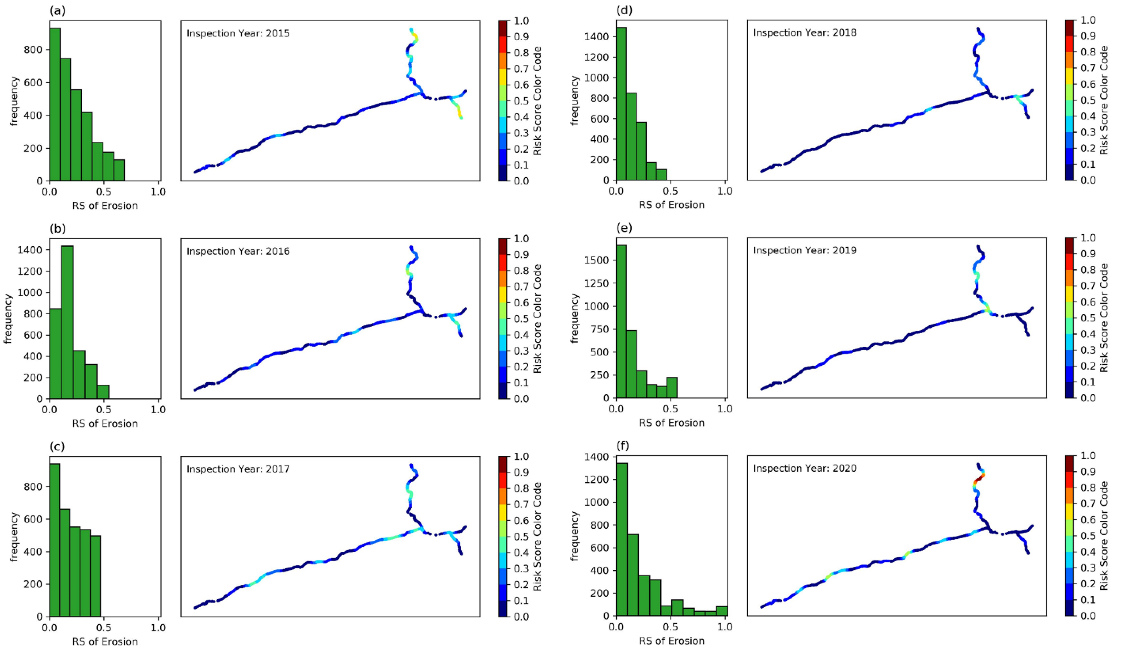
This section provides the results of applying the MDHP to the selected case study. Figure 6 provides the histogram of erosion RSs on paved ditches and the corresponding KDE results at the end of FY2015, FY2016, FY2017, and FY2018. Similarly, we calculated the RSs of the considered defects on the selected asset types (See Table 4) at the end of FY2015, FY2016, FY2017, and FY2018 to be used in the prediction. We used Silverman and nearest-neighbor-based methods to estimate the bandwidth of KDE, and the estimations were 7.93 to 2.01 km (4.93 and 1.25 miles), respectively. We used the average of the values in our analysis and chose 5 km (3.1 miles) for the kernel bandwidth.
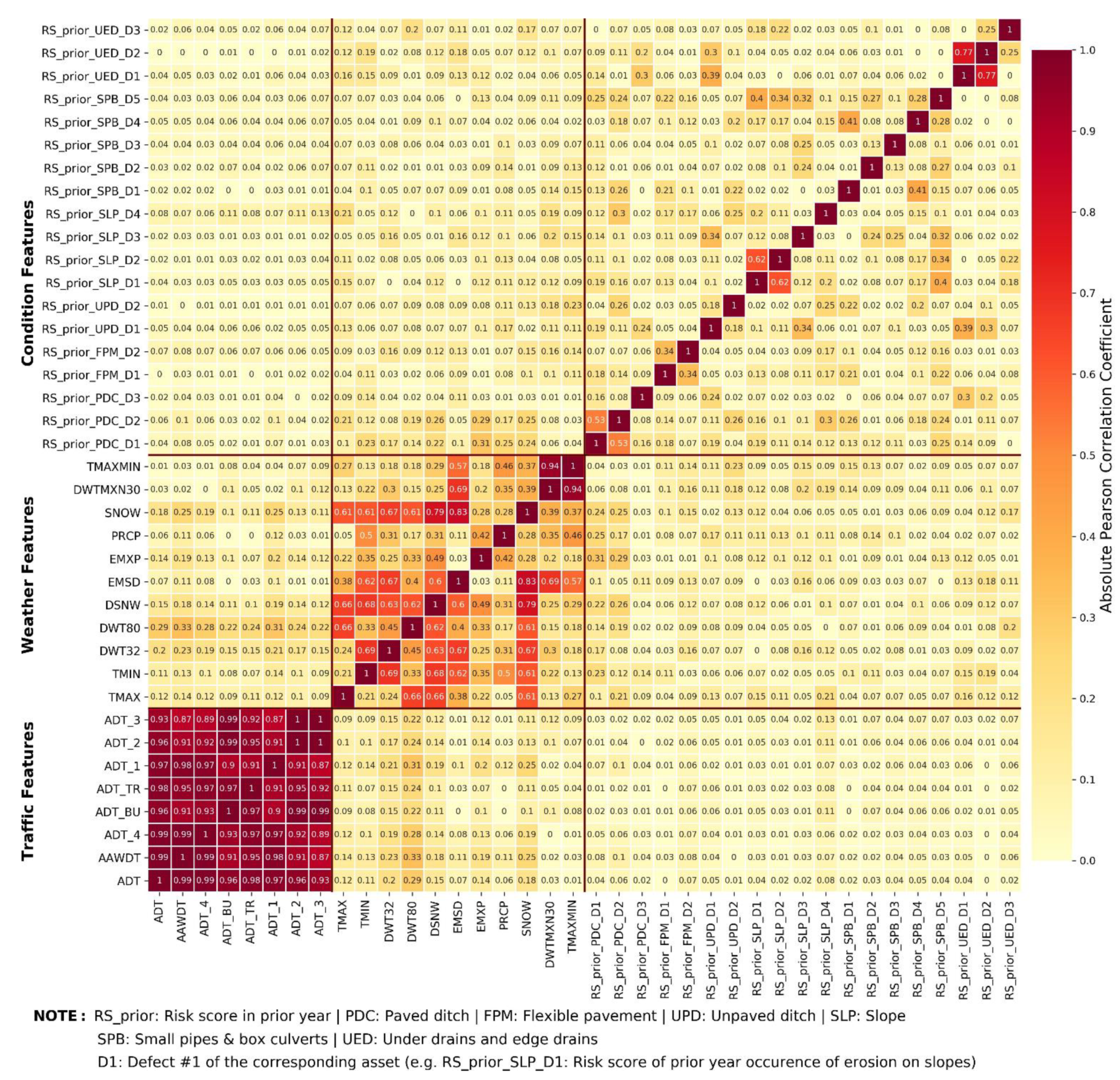
The considered contributing factors to the degradation of roadway assets in this study have different ranges and measurement units. Figure 7 provides a series of boxplots that visualize the different variations among continuous features. Later on, we used the min-max scaler to map all features to a range between 0 to 1 to prevent potential future biases of outcomes. To detect and remove multicollinearity in the input dataset, we investigated correlations between the input feature space. Figure 8 provides the pairwise absolute Pearson Correlation between continuous features. For example, the absolute Pearson correlation between ADT and AAWDT is 0.99 and between TMAXMIN and ADT is 0.01. Absolute Pearson correlation is a number between 0 and 1 that closer values to 1 represent more correlated parameters. As another example, in this study ADT and AAWDT were highly correlated. However, TMAXMIN and ADT has been very low correlated. Consequently, the data in Figure 8 show that only traffic attributes (ADT, AAWDT, ADT_4, ADT_BU, ADT_TR, ADT_1, ADT_2, and ADT_3) are highly correlated (i.e., their pairwise absolute Pearson correlation is greater than 0.9). Therefore, we reduced the continuous feature space by keeping ADT as the sole representative of traffic features.
Table 5 provides the Chi-square test results, or in other words, the dependencies among categorical features. The results show that M_71152 and M_72224 are highly correlated (i.e., the corresponding p-value is greater than 0.05). Therefore, we only kept M_72224, M_70141, M_70142, and M_72223 and removed M-71152 for future analysis.
Finally, Figure 9 presents the absolute point-biserial correlation coefficients between remaining categorical and continuous features. According to the results, none of the features are highly correlated and all features can be considered independent.
After reducing feature space and removing multicollinearity, we used the selected ML algorithms to predict RSs of erosion, obstruction, and cracking on paved ditches. The results of the models for erosion RSs are presented in Figure 10 as an example. In this figure, we are reporting the obtained coefficient of determination (R2), adjusted coefficient of determination (R2adj), and the Root Mean Square Error (RMSE). In addition, we are visualizing the observed vs. predicted Risk Score (RS) values in all considered algorithms on unseen data (i.e., testing set). For example, R2 for the developed model using Multivariate Linear Regression was 0.652. However, this value for Decision Tree model was 0.918. The higher value of R2 unveils the better performance of Decision Tree compared to Multivariate Linear Regression model.
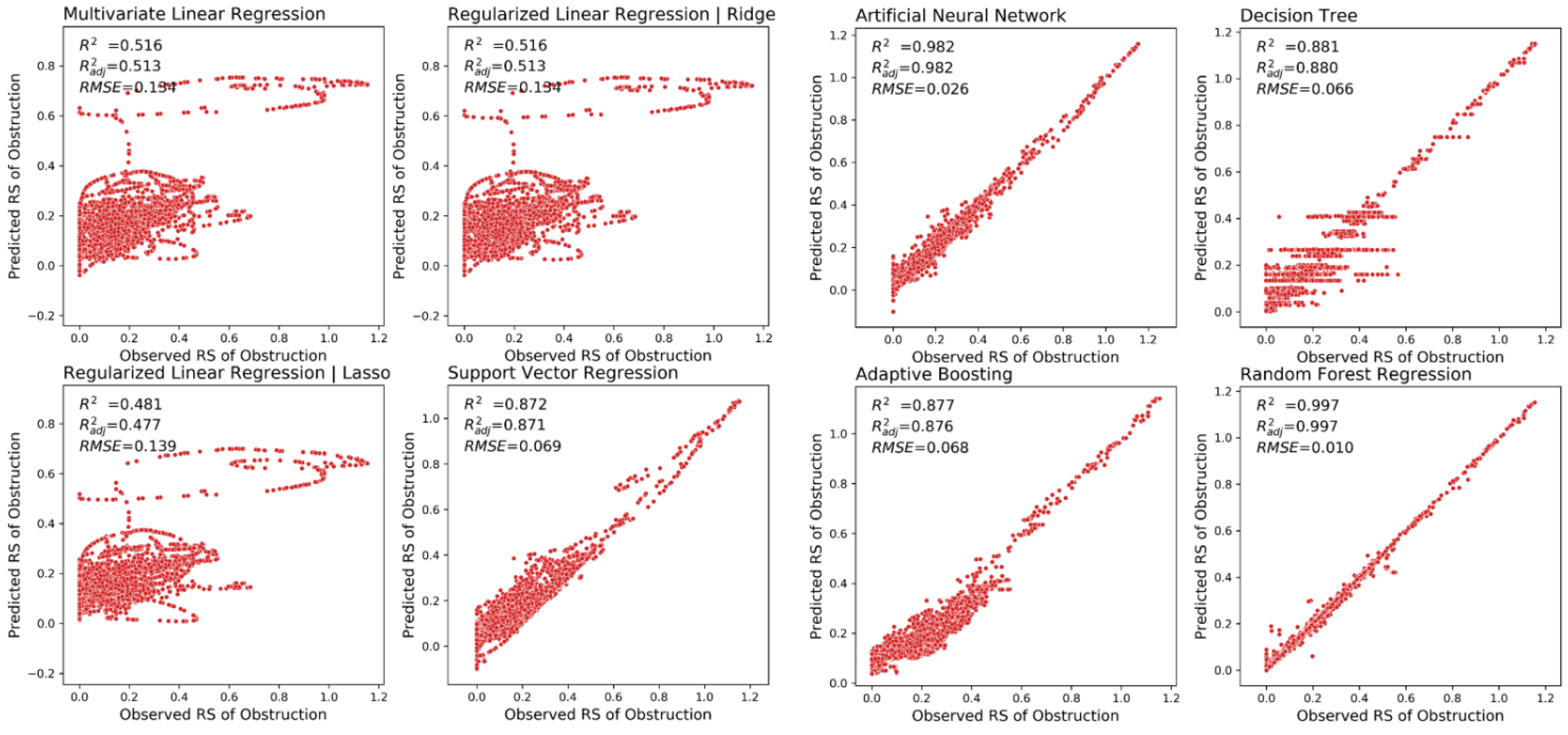
We used the same procedure to build prediction models for obstruction and cracking on paved ditches as well. Figure 11 and Figure 12 present the results of the developed models using different ML algorithms for obstruction and cracking respectively. Then, we summarized the training and testing scores (R2) of all of the considered models for the three considered defects in Table 6. The results indicate that the considered linear models (i.e., multilinear regression, Ridge, and Lasso) in all cases provided low R2 both in training and testing sets. Therefore, the models were incapable of capturing the patterns and relationships in the dataset. Consequently, this could be interpreted as the existence of nonlinear relationships among features and the need for nonlinear models. The obtained R2 of nonlinear models in both training and testing steps corroborates the interpretation.
Table 7 shows the results of k-fold cross-validation of the considered models when five is selected as the number of folds. In this table, for each selected ML algorithm, the minimum and maximum scores in the five folds of training and testing sets are provided. The cross-validation results show the narrow range of scores in all five folds of validation, which shows the lack of overfitting in all the developed models.
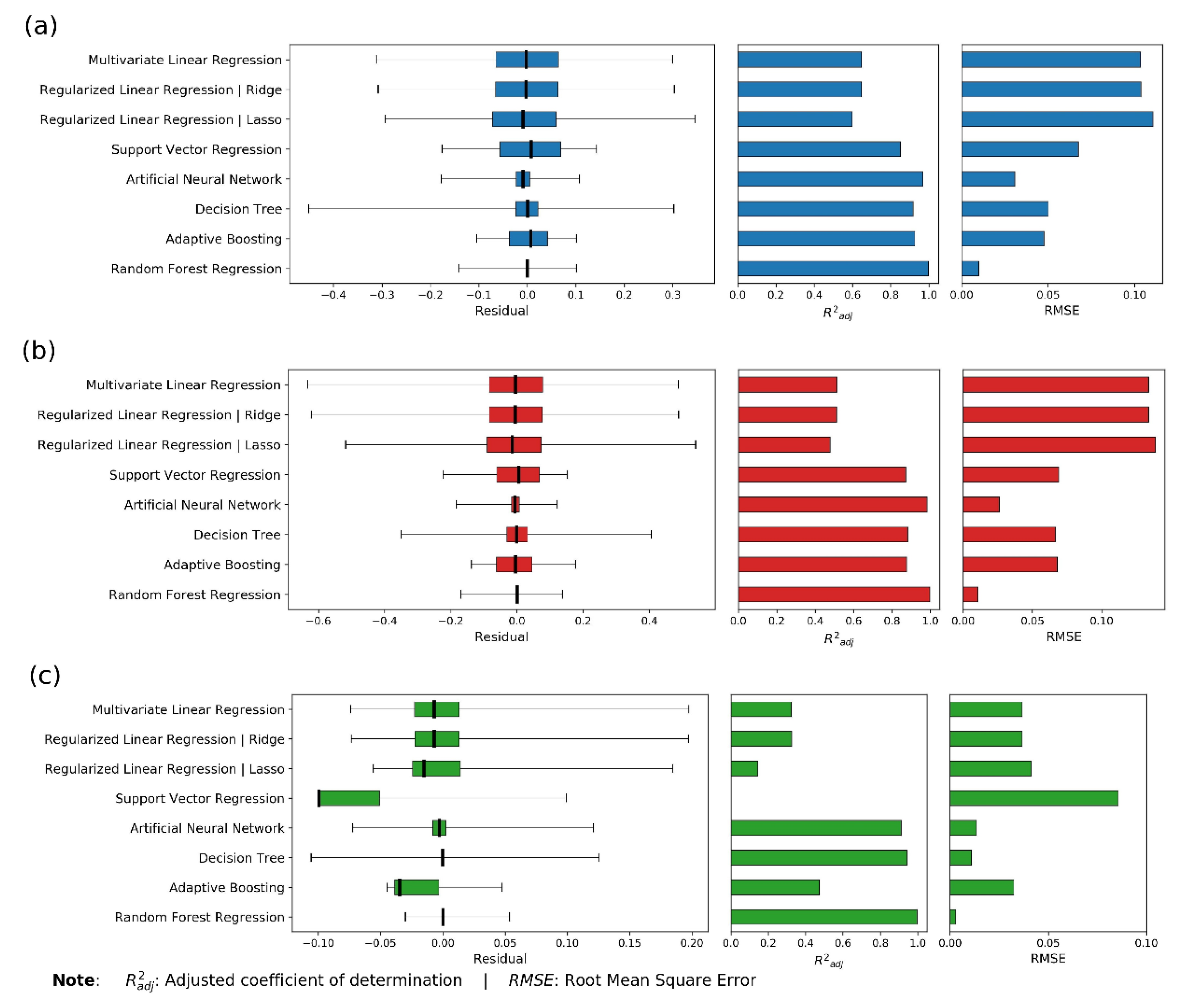
Additionally, a summary of the accuracy metrics for the corresponding prediction models is provided in Figure 13. This figure unveils that in all cases, the RFR provided the highest R2 values. Additionally, as shown in Figure 13, the values of RMSE for RFR models in three cases of erosion, obstruction, and cracking were 0.01, 0.01, and 0.03 respectively that were less than that of all other models. Therefore, the highest values of R2 and lowest values of RMSE highlight more accurate outcomes of RFR method among all the considered algorithms. Additionally, Figure 10 reveals that the predicted values using RFR are very close to the observed values in the considered dataset. Therefore, given the fact that all measurements pointed out the RFR as the best model for the considered case study, we selected RFR as the best fit and proceeded with this model for further analyses.
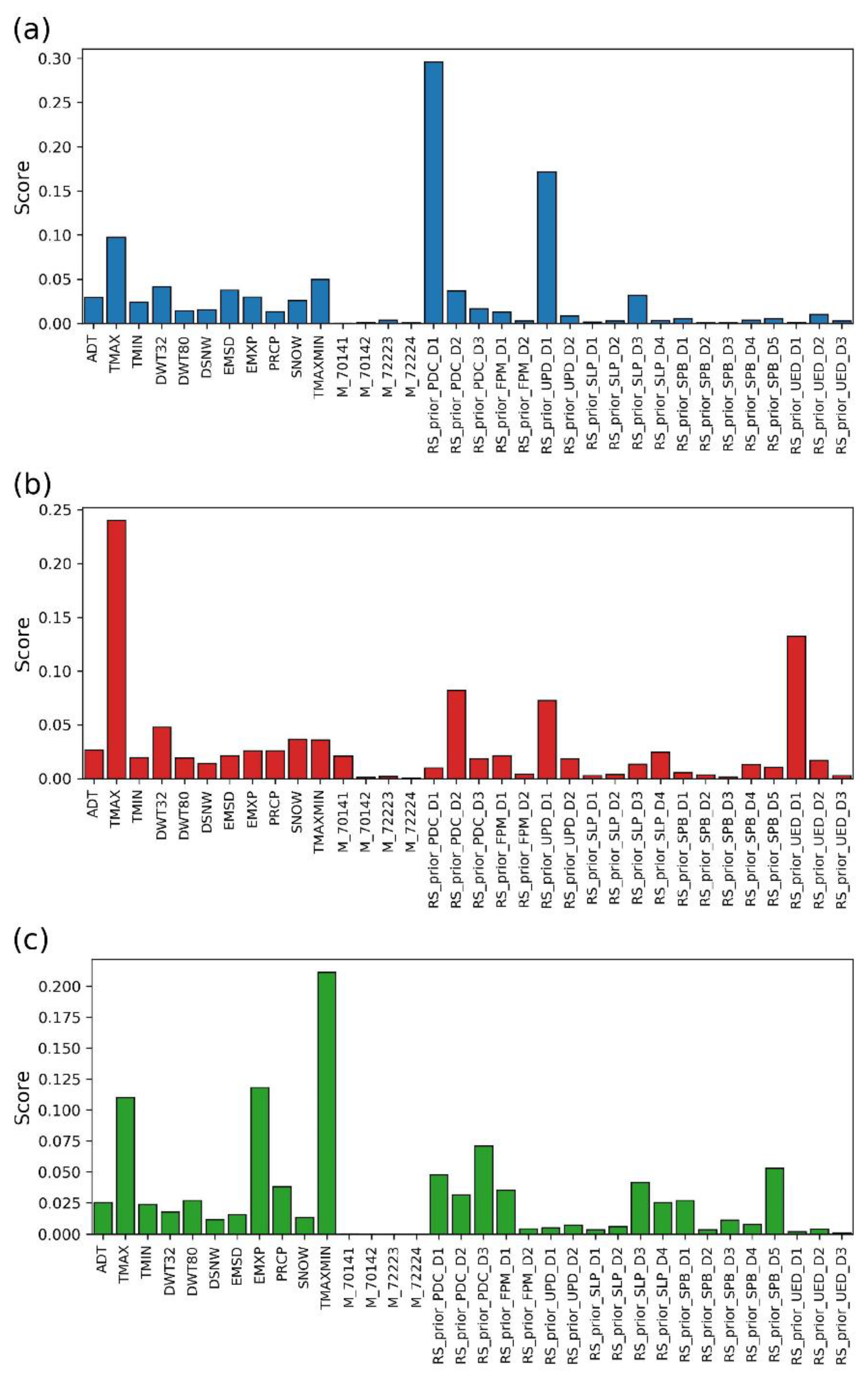
One of the best attributes of RFR is its capability in quantifying the contribution (i.e., importance) of each feature in the regression by providing a metric called importance score. To measure the importance of each contributing factor, most methods rely on the decrease in the accuracy when a permutation to a specific feature is performed. In this approach, when a feature is permuted, its original relationship within the decision trees with the final output is disturbed. Therefore, using the permuted feature along with the other non-permuted features might result in a decrease in the accuracy of predictions. This descent in accuracy is believed to be a realistic way of finding the importance of each feature. The more accuracy decrease can be interpreted as more contribution of that feature into regression [80]. We used this metric here to measure the importance of the considered features in our regression analysis. By utilizing RFR, our main goal is to let the model decide the most significant contributors among the wide range of potential candidates that we included in the framework, instead of subjectively selecting them beforehand. In this way, the important contributors might vary from asset to asset, which shows that our proposed framework respects the difference among the different highway assets’ nature.
We investigated the importance of each considered contributing factor to interpret their contribution to the regression using the aforementioned attribute of RFR. Figure 14 provides the obtained results in erosion, obstruction, and cracking predictions. This figure shows that paved ditch erosion RS in the prior year, the erosion of neighboring unpaved ditches, and maximum annual daily temperature (TMAX) contributed most to the predicted erosion RS. In addition, the importance of the annual average of daily max-min temperature difference (TMAXMIN) and the number of freezing days (DWT32) are considerable. The results confirm the interrelations between nearby assets and their importance on one another’s conditions. More importantly, the outcomes also highlight the higher contribution of short-term precipitation factors (e.g., EMXP: the maximum daily precipitation, and EMSD: the maximum annual daily snow) in the erosion of paved ditches in comparison to the long-term average annual precipitation (i.e., PRCP and SNOW). Finally, the results underline the small contribution of two of the maintenance works (M_72223: Concrete Patching/Repair and M_70142: Machine cleaning) in erosion RS of paved ditches out of the considered maintenance tasks.
Similarly, we investigated the importance of contributing factors in the prediction model of obstruction RSs on paved ditches. According to Figure 14, like erosion, the maximum annual daily temperature (TMAX) has a bold contribution to the values of obstruction RSs calculated by the model. Also, the contribution of the number of freezing days (DWT32), the annual average of daily max-min temperature difference (TMAXMIN), and total annual snow depth were significant. Furthermore, in this case, long-term precipitation features (i.e., PRCP and SNOW) had more contribution in predicting obstruction RSs compared to the short-term precipitation features (EMSD and EMXP). In addition, the contribution of the drain outlet defect in the prior year (RS_prior_UED_D1) in the vicinity of paved ditches was noticeable. The reason for this contribution could be attributed to the downstream blockage resulted from defected under drains and edge drains outlet and settlement of debris and obstruction in the upstream ditches. The figure also highlights the contribution of the condition of other neighboring assets, such as erosion on unpaved ditches and lower-slope issue on slopes on calculating paved ditch obstruction RSs.
Figure 14c reveals that TMAX and TMAXMIN that represent the temperature features and correspond to temperature harshness in a region contributed significantly to predicted cracking RSs. Besides, the next rank belongs to EMXP which is a short-term precipitation feature. This figure also unveils the importance of prior year cracking, erosion, and obstruction RSs in the next year cracking RSs on paved ditches. Ultimately, the results show that the condition of nearby assets contributed to the predicted RSs as well.
To assess the performance of the selected model in its implementation, the RSs at the end of FY2015, FY2016, FY2017, FY2018, and FY2019 as well as all contributing factors in FY2016, FY2017, FY2018, and FY2019 are utilized to build the prediction model. It is worth mentioning that the data is first is split into training and testing sets and all validation procedures are performed. Then, the model is used to predict RSs in FY2020 when RSs at the end of FY2019 and contributing factors in FY2020 are the inputs of the model. Later on, the performance of the hotspot prediction is assessed considering the actual observations of RSs at the end of FY2020. With respect to the scenario introduced for assessing the performance of the proposed framework in its implementation, we used RFR to develop a RS prediction model for erosion on paved ditches. Figure 15 displays the spatial distribution of erosion RSs that provides a comparison between observed and predicted RSs at the end of FY2020 in different mile markers (i.e., segments) of the case study. It can visually be concluded that there is an acceptable correlation between the longitudinal profile of the locations of predicted and observed RSs in both cases. Since there is not any specific threshold available that specifies high and low values of RSs, we used the Jenks method to cluster RSs into similar groups in terms of their severity [81]. In another word, this method results in a cut-off threshold that clearly divides RSs into two categories (hotspots and coldspots), which could help us better document and investigate the match between predicted and observed RSs. In this context, hotspots refer to the location of roadways with a higher density of defects while coldspots show the parts of roads with a fewer number of defects. We summarized the results of this task in Figure 16. This figure illustrates hotspots and coldspots with respect to the calculated Jenks threshold of 0.3 applied on the dataset. The match percentage between observed and predicted RSs on all segments according to this categorization is 81.9 percent. This number demonstrates that our prediction framework offered an acceptable accuracy in predicting the location of hotspots and coldspots in a year ahead. We performed a similar procedure for obstruction and cracking and gained 96.2 and 96.1 match percentages, respectively, both of which further providing promising results in localizing the hotspots in a future year.

6. Conclusions

In this paper, we proposed a Multi-asset Defect Hotspot Predictor (MDHP), a multi-asset prediction framework that forecasts the susceptibility of roadway assets. We then used a case study of 389 km of I-81, I-77, and I-381 Interstate highways in the US to evaluate the proposed framework’s performance. The MDHP provided significant accuracy in forecasting the hotspots of erosion, obstruction, and cracking defects on paved ditches in our case study. Furthermore, the outcomes highlighted an interrelation between adjacent assets and their contribution to future defects. For instance, the effect of the downstream drain outlet damages on the obstruction of upstream paved ditches was identified. As another example, prior year erosion in unpaved ditches and lower-slopes, contributed to the erosion in the paved ditches. The findings of this study also considers the disparate nature of highway assets using a data-driven approach in identifying major contributors in defecting different assets.
This study provides decision-makers with a prediction tool to identify parts of roadways that are prone to different defects. Hence, agencies can better plan and prioritize maintenance activities based on the outcomes of the proposed models. Furthermore, the proposed methodology offers an integrated estimator of defects’ probability for multiple assets compared to the previous methods predicting individual asset’s condition in isolation. Consequently, it has the potential of benefiting risk mitigation plans for the highway infrastructure. Ultimately, the proposed framework can also help agencies to optimize and prioritize their future inspections with a targeted strategy to focus on locations with a higher probability of defects.
Even though the proposed framework does not have any constraints on the scope of inputs, we only used five years of information and considered six asset types due to data availability. Therefore, it is suggested that future studies consider applying the methodology to other road assets and cover a more extended temporal content. Besides, the application of the MDHP method on other linear or network infrastructures such as sewers, water networks, and railroads would make an interesting research direction.

Author Contributions

Conceptualization, A.K., O.S. and H.T.; Data curation, A.K. and S.S.; Formal analysis, A.K.; Funding acquisition, O.S.; Methodology, A.K., O.S. and S.S.; Project administration, O.S.; Resources, O.S.; Software, A.K.; Supervision, O.S. and H.T.; Validation, A.K., S.S. and H.T.; Visualization, A.K. and O.S.; Writing—original draft, A.K. and O.S.; Writing—review & editing, O.S., S.S. and H.T. All authors have read and agreed to the published version of the manuscript.

Funding

This research was partially funded by VIRGINIA DEPARTMENT OF TRANSPORTATION (VDOT) and LEIDOS.

Institutional Review Board Statement

Not applicable.

Informed Consent Statement

Not applicable.

Data Availability Statement

Some or all data, models, or code generated or used during the study are proprietary or confidential in nature and may only be provided with the permission of the Sponsor.

Acknowledgments

We would like to thank the Virginia Department of Transportation (VDOT) for sponsoring and supporting this research project, and the Bristol district staff for providing relevant data for the modeling. We would also like to acknowledge the LEIDOS research teammate members for their significant contribution to this study. Additionally, we would like to appreciate all information and valuable feedback that Charles D. Gantt provided on the maintenance data utilized in this study.

Conflicts of Interest

The authors declare no conflict of interest.

References

  1. NASEM. Critical Issues in Transportation 2019. In The National Academies of Science, Engineering & Medicine; The National Academies Press: Washington, DC, USA, 2019. [Google Scholar]
  2. AASHTO. AASHTO Transportation Asset Management Guide: A Focus on Implementation; AASHTO: Washington, DC, USA, 2011. [Google Scholar]
  3. Frangopol, D.M.; Dong, Y.; Sabatino, S. Bridge life-cycle performance and cost: Analysis, prediction, optimization and decision-making. Struct. Infrastruct. Eng. 2017, 13, 1239–1257. [Google Scholar] [CrossRef]
  4. Kobayashi, K.; Kaito, K. Big data-based deterioration prediction models and infrastructure management: Towards assetmetrics. Struct. Infrastruct. Eng. 2017, 13, 84–93. [Google Scholar] [CrossRef]
  5. Shoghli, O.; De La Garza, J.M. A multi-objective decision-making approach for the sustainable maintenance of roadways. In Construction Research Congress; American Society of Civil Engineers: Reston, VA, USA, 2016; pp. 1424–1434. [Google Scholar]
  6. Piryonesi, S.M.; El-Diraby, T. Climate change impact on infrastructure: A machine learning solution for predicting pavement condition index. Constr. Build. Mater. 2021, 306, 124905. [Google Scholar] [CrossRef]
  7. Pan, Y.; Zhang, L. A BIM-data mining integrated digital twin framework for advanced project management. Autom. Constr. 2021, 124, 103564. [Google Scholar] [CrossRef]
  8. Falls, L.C.; Haas, R.; Tighe, S. Asset service index as integration mechanism for civil infrastructure. Transp. Res. Rec. 2006, 1957, 1–7. [Google Scholar] [CrossRef]
  9. Coffey, S.; Park, S. Observational study on the pavement performance effects of shoulder rumble strip on shoulders. Int. J. Pavement Res. Technol. 2016, 9, 255–263. [Google Scholar] [CrossRef] [Green Version]
  10. Ghabchi, R.; Zaman, M.; Khoury, N.; Kazmee, H.; Solanki, P. Effect of gradation and source properties on stability and drainability of aggregate bases: A laboratory and field study. Int. J. Pavement Eng. 2013, 14, 274–290. [Google Scholar] [CrossRef]
  11. Karimzadeh, A.; Sabeti, S.; Burde, A.; Tabkhi, H.; Shoghli, O. Spatial-Temporal Deterioration of Multiple Highway Assets: A Correlational Study. In Proceedings of the ASCE Construction Research Congress (CRC)—2020, Tempe, AZ, USA, 8–10 March 2020. [Google Scholar]
  12. Abaza, K.A. Empirical Markovian-based models for rehabilitated pavement performance used in a life cycle analysis approach. Struct. Infrastruct. Eng. 2017, 13, 625–636. [Google Scholar] [CrossRef]
  13. Chimba, D.; Emaasit, D.; Allen, S.; Hurst, B.; Nelson, M. Factors affecting median cable barrier crash frequency: New insights. J. Transp. Saf. Secur. 2014, 6, 62–77. [Google Scholar] [CrossRef]
  14. Elwakil, E.; Eweda, A.; Zayed, T. Modelling the effect of various factors on the condition of pavement marking. Struct. Infrastruct. Eng. 2014, 10, 93–105. [Google Scholar] [CrossRef]
  15. Halmen, C.; Trejo, D.; Folliard, K. Service Life of Corroding Galvanized Culverts Embedded in Controlled Low-Strength Materials. J. Mater. Civ. Eng. 2008, 20, 366–374. [Google Scholar] [CrossRef]
  16. Immaneni, V.P.; Hummer, J.E.; Rasdorf, W.J.; Harris, E.A.; Yeom, C. Synthesis of sign deterioration rates across the United States. J. Transp. Eng. 2009, 135, 94–103. [Google Scholar] [CrossRef]
  17. Malyuta, D.A. Analysis of Factors Affecting Pavement Markings and Pavement Marking Retroreflectivity in Tennessee Highways. University of Tennessee at Chattanooga. Ph.D. Thesis, University of Tennessee at Chattanooga, Chattanooga, TN, USA, 2015. [Google Scholar]
  18. Sitzabee, W.E.; White, E.D.; Dowling, A.W. Degradation modeling of polyurea pavement markings. Public Work. Manag. Policy 2012, 18, 185–199. [Google Scholar] [CrossRef]
  19. Mills LN, O.; Attoh-Okine, N.O.; McNeil, S. Developing pavement performance models for Delaware. Transp. Res. Rec. 2012, 2304, 97–103. [Google Scholar] [CrossRef]
  20. Saha, P.; Ksaibati, K.; Atadero, R. Developing Pavement Distress Deterioration Models for Pavement Management System Using Markovian Probabilistic Process. Adv. Civ. Eng. 2017, 2017, 8292056. [Google Scholar] [CrossRef] [Green Version]
  21. Pantuso, A.; Flintsch, G.W.; Katicha, S.W.; Loprencipe, G. Development of network-level pavement deterioration curves using the linear empirical Bayes approach. Int. J. Pavement Eng. 2019, 22, 780–793. [Google Scholar] [CrossRef] [Green Version]
  22. Karimzadeh, A.; Sabeti, S.; Shoghli, O. Optimal Clustering of Pavement Segments Using K-Prototype Algorithm in a High-Dimensional Mixed Feature Space. J. Manag. Eng. 2021, 37, 04021022. [Google Scholar] [CrossRef]
  23. Anyala, M.; Odoki, J.; Baker, C. Hierarchical asphalt pavement deterioration model for climate impact studies. Int. J. Pavement Eng. 2014, 15, 251–266. [Google Scholar] [CrossRef]
  24. Bannour, A.; El Omari, M.; Lakhal, E.K.; Afechkar, M.; Benamar, A.; Joubert, P. Optimization of the maintenance strategies of roads in Morocco: Calibration study of the degradations models of the highway development and management (HDM-4) for flexible pavements. Int. J. Pavement Eng. 2017, 20, 245–254. [Google Scholar] [CrossRef]
  25. Ford, K.M.; Arman, M.; Labi, S.; Sinha, K.C.; Thompson, P.; Shirole, A.; Li, Z. Estimating Life Expectancies of Highway Assets—Volume 2: Final Report; Transportation Research Board, National Academy of Sciences: Washington, DC, USA, 2012. [Google Scholar]
  26. Hong, F.; Prozzi, J.A. Roughness model accounting for heterogeneity based on in-service pavement performance data. J. Transp. Eng. 2010, 136, 205–213. [Google Scholar] [CrossRef]
  27. Labi, S.; Sinha, K.C. Measures of short-term effectiveness of highway pavement maintenance. J. Transp. Eng. 2003, 129, 673–683. [Google Scholar] [CrossRef]
  28. Prozzi, J.A.; Serigos, P.A.; Kim, M.Y.; Xu, H. Deterioration Modelling of Preventive Maintenance Treatments for Flexible Pavements; University of Texas at Austin: Austin, TX, USA, 2017. [Google Scholar]
  29. Ré, J.; Miles, J.; Carlson, P. Analysis of in-service traffic sign retroreflectivity and deterioration rates in Texas. Transp. Res. Rec. 2011, 2258, 88–94. [Google Scholar] [CrossRef]
  30. Wang, C.; Wang, Z.; Tsai, Y.-C. Piecewise Multiple Linear Models for Pavement Marking Retroreflectivity Prediction Under Effect of Winter Weather Events. Transp. Res. Rec. 2016, 2551, 52–61. [Google Scholar] [CrossRef]
  31. Karimzadeh, A.; Shoghli, O. Predictive analytics for roadway maintenance: A review of current models, challenges, and opportunities. Civ. Eng. J. 2020, 6, 602–625. [Google Scholar] [CrossRef] [Green Version]
  32. Hunt, P.D.; Bunker, J.M. Study of site-specific roughness progression for a bitumen-sealed unbound granular pavement network. Transp. Res. Rec. 2003, 1819, 273–281. [Google Scholar] [CrossRef] [Green Version]
  33. Von Quintus, H.L.; Eltahan, A.; Yau, A. Smoothness models for hot-mix asphalt-surfaced pavements: Developed from long-term pavement performance program data. Transp. Res. Rec. 2001, 1764, 139–156. [Google Scholar] [CrossRef]
  34. Kargah-Ostadi, N.; Stoffels, S.M. Framework for development and comprehensive comparison of empirical pavement performance models. J. Transp. Eng. 2015, 141, 04015012. [Google Scholar] [CrossRef]
  35. Swargam, N. Development of a Neural Network Approach for the Assessment of the Performance of Traffic Sign Retroreflectivity. Master’s Thesis, Lousiana State University, Civil and Environmental Engineering, Baton Rouge, LA, USA, 2004. [Google Scholar]
  36. Haider, S.W.; Chatti, K. Effect of design and site factors on fatigue cracking of new flexible pavements in the LTPP SPS-1 experiment. Int. J. Pavement Eng. 2009, 10, 133–147. [Google Scholar] [CrossRef]
  37. Karwa, V.; Donnell, E.T. Predicting pavement marking retroreflectivity using artificial neural networks: Exploratory analysis. J. Transp. Eng. 2011, 137, 91–103. [Google Scholar] [CrossRef]
  38. Karlaftis, A.G.; Badr, A. Predicting asphalt pavement crack initiation following rehabilitation treatments. Transp. Res. Part C Emerg. Technol. 2015, 55, 510–517. [Google Scholar] [CrossRef]
  39. Marcelino, P.; de Lurdes Antunes, M.; Fortunato, E.; Gomes, M.C. Machine learning approach for pavement performance prediction. Int. J. Pavement Eng. 2021, 22, 341–354. [Google Scholar] [CrossRef]
  40. Wang, W.-C.; Chau, K.-W.; Qiu, L.; Chen, Y.-B. Improving forecasting accuracy of medium and long-term runoff using artificial neural network based on EEMD decomposition. Environ. Res. 2015, 139, 46–54. [Google Scholar] [CrossRef] [PubMed]
  41. Chopra, T.; Parida, M.; Kwatra, N.; Chopra, P. Development of Pavement Distress Deterioration Prediction Models for Urban Road Network Using Genetic Programming. Adv. Civ. Eng. 2018, 2018, 1253108. [Google Scholar] [CrossRef] [Green Version]
  42. Sanabria, N.; Valentin, V.; Bogus, S.; Zhang, G.; Kalhor, E. Comparing Neural Networks and Ordered Probit Models for Forecasting Pavement Condition in New Mexico. In Proceedings of the Transportation Research Board 96th Annual Meeting, Washington, DC, USA, 8–12 January 2017. [Google Scholar]
  43. Proctor, G.; Varma, S. Risk-Based Transportation Asset Management: Evaluating Threats, Capitalizing on Opportunities: Report 1: Overview of Risk Management; National Academy of Sciences: Washington, DC, USA, 2012. [Google Scholar]
  44. Renn, O. Risk Governance: Coping with Uncertainty in a Complex World; Earthscan: London, UK, 2008. [Google Scholar]
  45. Kuter, N.; Kuter, S. Investigation of wildfire at forested landscapes: A novel contribution to nonparametric density mapping at regional scale. Appl. Ecol. Environ. Res. 2018, 16, 4701–4716. [Google Scholar] [CrossRef]
  46. Massada, A.B.; Radeloff, V.C.; Stewart, S.I.; Hawbaker, T.J. Wildfire risk in the wildland–urban interface: A simulation study in northwestern Wisconsin. For. Ecol. Manag. 2009, 258, 1990–1999. [Google Scholar] [CrossRef]
  47. Millington, J.; Romero-Calcerrada, R.; Wainwright, J.; Perry, G. An agent-based model of Mediterranean agricultural land-use/cover change for examining wildfire risk. J. Artif. Soc. Soc. Simul. 2008, 11, 4. [Google Scholar]
  48. Gaull, B.; Michael-Leiba, M.; Rynn, J. Probabilistic earthquake risk maps of Australia. Aust. J. Earth Sci. 1990, 37, 169–187. [Google Scholar] [CrossRef]
  49. Erdogan, S. Explorative spatial analysis of traffic accident statistics and road mortality among the provinces of Turkey. J. Saf. Res. 2009, 40, 341–351. [Google Scholar] [CrossRef]
  50. Rahman, M.K.; Crawford, T.; Schmidlin, T.W. Spatio-temporal analysis of road traffic accident fatality in Bangladesh integrating newspaper accounts and gridded population data. GeoJournal 2018, 83, 645–661. [Google Scholar] [CrossRef]
  51. Wang, J.; Wang, X. An ontology-based traffic accident risk mapping framework. In Proceedings of the International Symposium on Spatial and Temporal Databases, Minneapolis, MN, USA, 24–26 August 2011. [Google Scholar]
  52. Hunt, R.E. Slope failure risk mapping for highways: Methodology and case history. Transp. Res. Rec. 1992, 1343, 42–51. [Google Scholar]
  53. Sohn, J. Evaluating the significance of highway network links under the flood damage: An accessibility approach. Transp. Res. Part A Policy Pract. 2006, 40, 491–506. [Google Scholar] [CrossRef]
  54. Wright, L.; Chinowsky, P.; Strzepek, K.; Jones, R.; Streeter, R.; Smith, J.B.; Mayotte, J.-M.; Powell, A.; Jantarasami, L.; Perkins, W. Estimated effects of climate change on flood vulnerability of US bridges. Mitig. Adapt. Strateg. Glob. Change 2012, 17, 939–955. [Google Scholar] [CrossRef] [Green Version]
  55. Anderson, C.J.; Claman, D.; Mantilla, R. Iowa’s Bridge and Highway Climate Change and Extreme Weather Vulnerability Assessment Pilot; Institute for Transportation: Ames, IA, USA, 2015. [Google Scholar]
  56. Lu, D. Pavement Flooding Risk Assessment and Management in the Changing Climate. Ph.D. Thesis, University of Waterloo, Waterloo, ON, Canada, 2020. [Google Scholar]
  57. da Silva AS, A.; Stosic, B.; Menezes RS, C.; Singh, V.P. Comparison of Interpolation Methods for Spatial Distribution of Monthly Precipitation in the State of Pernambuco, Brazil. J. Hydrol. Eng. 2019, 24, 04018068. [Google Scholar] [CrossRef]
  58. Frazier, A.G.; Giambelluca, T.W.; Diaz, H.F.; Needham, H.L. Comparison of geostatistical approaches to spatially interpolate month-year rainfall for the Hawaiian Islands. Int. J. Climatol. 2016, 36, 1459–1470. [Google Scholar] [CrossRef] [Green Version]
  59. Plouffe, C.C.; Robertson, C.; Chandrapala, L. Comparing interpolation techniques for monthly rainfall mapping using multiple evaluation criteria and auxiliary data sources: A case study of Sri Lanka. Environ. Model. Softw. 2015, 67, 57–71. [Google Scholar] [CrossRef]
  60. Anderson, T.K. Kernel density estimation and K-means clustering to profile road accident hotspots. Accid. Anal. Prev. 2009, 41, 359–364. [Google Scholar] [CrossRef]
  61. Silverman, B.W. Density Estimation for Statistics and Data Analysis; CRC Press: Boca Raton, FL, USA, 1986; Volume 26. [Google Scholar]
  62. Chainey, S.; Ratcliffe, J. GIS and Crime Mapping; John Wiley & Sons: Hoboken, NJ, USA, 2013. [Google Scholar]
  63. Aksoy, S.; Haralick, R.M. Feature normalization and likelihood-based similarity measures for image retrieval. Pattern Recognit. Lett. 2001, 22, 563–582. [Google Scholar] [CrossRef] [Green Version]
  64. Yoo, W.; Mayberry, R.; Bae, S.; Singh, K.; He, Q.P.; Lillard, J.W., Jr. A study of effects of multicollinearity in the multivariable analysis. Int. J. Appl. Sci. Technol. 2014, 4, 9. [Google Scholar]
  65. Leggetter, C.; Woodland, P.C. Speaker adaptation of continuous density HMMs using multivariate linear regression. Int. Conf. Spok. Lang. Process. 1994, 94, 451–454. [Google Scholar]
  66. Yuan, M.; Ekici, A.; Lu, Z.; Monteiro, R. Dimension reduction and coefficient estimation in multivariate linear regression. J. R. Stat. Soc. Ser. B 2007, 69, 329–346. [Google Scholar] [CrossRef]
  67. Friedman, J.; Hastie, T.; Tibshirani, R. The Elements of Statistical Learning (Vol. 1): Springer Series in Statistics New York; Springer: New York, NY, USA, 2001. [Google Scholar]
  68. Clarke, S.M.; Griebsch, J.H.; Simpson, T.W. Analysis of support vector regression for approximation of complex engineering analyses. J. Mech. Des. 2005, 127, 1077–1087. [Google Scholar] [CrossRef]
  69. Wu, C.-H.; Tzeng, G.-H.; Lin, R.-H. A Novel hybrid genetic algorithm for kernel function and parameter optimization in support vector regression. Expert Syst. Appl. 2009, 36, 4725–4735. [Google Scholar] [CrossRef]
  70. Cohen, S.; Intrator, N. A study of ensemble of hybrid networks with strong regularization. In Proceedings of the International Workshop on Multiple Classifier Systems, Guildford, UK, 11–13 June 2003. [Google Scholar]
  71. Yilmaz, I.; Kaynar, O. Multiple regression, ANN (RBF, MLP) and ANFIS models for prediction of swell potential of clayey soils. Expert Syst. Appl. 2011, 38, 5958–5966. [Google Scholar] [CrossRef]
  72. Tso, G.K.; Yau, K.K. Predicting electricity energy consumption: A comparison of regression analysis, decision tree and neural networks. Energy 2007, 32, 1761–1768. [Google Scholar] [CrossRef]
  73. Schapire, R.E. The boosting approach to machine learning: An overview. In Nonlinear Estimation and Classification; Springer: Berlin/Heidelberg, Germany, 2003; pp. 149–171. [Google Scholar]
  74. Karabulut, E.M.; Ibrikci, T. Analysis of cardiotocogram data for fetal distress determination by decision tree based adaptive boosting approach. J. Comput. Commun. 2014, 2, 32–37. [Google Scholar] [CrossRef] [Green Version]
  75. Yaseen, Z.M.; Sulaiman, S.O.; Deo, R.C.; Chau, K.-W. An enhanced extreme learning machine model for river flow forecasting: State-of-the-art, practical applications in water resource engineering area and future research direction. J. Hydrol. 2019, 569, 387–408. [Google Scholar] [CrossRef]
  76. Breiman, L. Random Forests. Mach. Learn. 2001, 45, 5–32. [Google Scholar] [CrossRef] [Green Version]
  77. Fushiki, T. Estimation of prediction error by using K-fold cross-validation. Stat. Comput. 2011, 21, 137–146. [Google Scholar] [CrossRef]
  78. Suen, Y.L.; Melville, P.; Mooney, R.J. Combining bias and variance reduction techniques for regression trees. In Proceedings of the European Conference on Machine Learning, Porto, Portugal, 3–7 October 2005. [Google Scholar]
  79. VDOT. Bundled Interstate Maintenance Services (BIMS): Instructions, Asset and Activity Codes for Reports Manual, Virginia Department of Transportation (VDOT); ProQuest LLC: Ann Arbor, MI, USA, 2014.
  80. Strobl, C.; Boulesteix, A.-L.; Zeileis, A.; Hothorn, T. Bias in random forest variable importance measures: Illustrations, sources and a solution. BMC Bioinform. 2007, 8, 25. [Google Scholar] [CrossRef] [Green Version]
  81. North, M.A. A method for implementing a statistically significant number of data classes in the Jenks algorithm. In Proceedings of the 2009 Sixth International Conference on Fuzzy Systems and Knowledge Discovery, Tianjin, China, 14–16 August 2009. [Google Scholar]
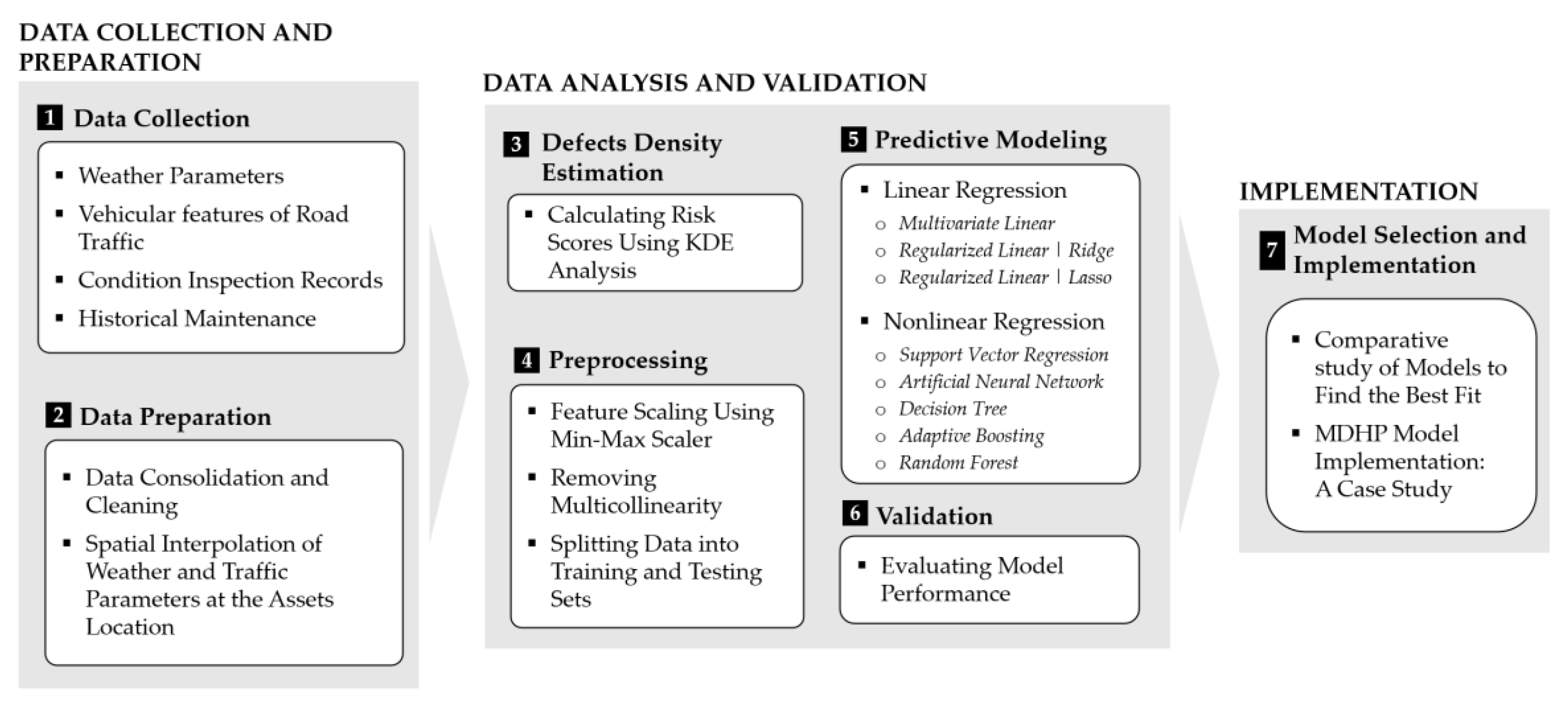
Figure 1. The Framework of the proposed Multi-asset Defect Hotspot Predictor (MDHP).
Sustainability 14 04979 g001
Figure 2. (a) Spatial distribution of observed defects on paved ditches (b) Corresponding Risk Scores (RSs) of defects based on KDE analysis.
Sustainability 14 04979 g002
Figure 3. The process for Risk Score (RS) prediction of a defect (erosion) at the location of a segment (Segment i) for an asset class (paved ditch) by use of previous year(s) data and incorporation of the impact of the nearby assets.
Sustainability 14 04979 g003
Figure 4. ANN-MLP structure used in the study.
Sustainability 14 04979 g004
Figure 5. Location of the roadways in the case study that includes 389 km of I-81, I-77, and I-381 Interstate highways in the state of Virginia.
Sustainability 14 04979 g005
Figure 6. Histograms and spatial distributions of erosion RSs in different years of inspection (a) FY2015 (b) FY2016 (c) FY2017 (d) FY2018 (e) FY2019 (f) FY2020.
Sustainability 14 04979 g006
Figure 7. Boxplots of continuous features: (a) traffic features, (b) temperature parameters, (c) precipitations records (d) duration of extreme weather events.
Sustainability 14 04979 g007
Figure 8. Absolute Pearson correlation matrix of continuous features.
Sustainability 14 04979 g008
Figure 9. Absolute point-biserial correlation matrix between continuous and categorical features.
Sustainability 14 04979 g009
Figure 10. Observed versus predicted erosion RSs using considered algorithms in the testing set (R2: Coefficient of determination, R2adj: Adjusted coefficient of determination, RMSE: Root Mean Square Error).
Sustainability 14 04979 g010
Figure 11. Observed versus predicted obstruction RSs using considered algorithms in the testing set (R2: Coefficient of determination, R2adj: Adjusted coefficient of determination, RMSE: Root Mean Square Error).
Sustainability 14 04979 g011
Figure 12. Observed versus predicted cracking RSs using considered algorithms in the testing set (R2: Coefficient of determination, R2adj: Adjusted coefficient of determination, RMSE: Root Mean Square Error).
Sustainability 14 04979 g012
Figure 13. Comparison of models’ accuracy metrics (a) prediction models for erosion RSs (b) prediction models for obstruction RSs (c) prediction models for cracking RSs (R2adj: Adjusted coefficient of determination, RMSE: Root Mean Square Error).
Sustainability 14 04979 g013
Figure 14. Importance feature scores in the RFR model for predicting RSs of defects: (a) erosion (b) obstruction (c) cracking.
Sustainability 14 04979 g014
Figure 15. Longitudinal distribution of RSs of erosion on paved ditches all over case study roadways at the end of FY2020.
Sustainability 14 04979 g015
Figure 16. Match percentage of (a) observed versus (b) predicted RSs of erosion on paved ditches at the end of FY2020.
Sustainability 14 04979 g016
Table 1. Weather parameters considered in the study.
IndexParameterDefinition
1TMAXAnnual maximum daily temperature (°C)
2TMINAnnual minimum daily temperature (°C)
3TMAXMINAnnual average of daily max-min temperature difference (°C)
4DWT32Number of days with minimum temperature < 0 °C (32 °F) in a year
5DWT80Number of days with maximum temperature > 26.7 °C (80 °F) in a year
6DWTMXN30Number of days with Tmax-Tmin > 16.7 °C (30 °F) in a year
7DSNWNumber of days with snow depth > 2.54 cm (1 inch) in a year
8EMSDMaximum annual daily snow depth (cm)
9EMXPMaximum annual daily precipitation depth (cm)
10PRCPTotal annual precipitation (cm)
11SNOWTotal annual snow depth (cm)
Table 2. Vehicular features of road traffic considered in the study.
IndexParameterDefinition
1ADTAverage daily traffic (number of vehicles per day)
2AAWDTAverage annual weekday traffic (number of vehicles per day)
3ADT_4Average daily traffic of 4-tire vehicles (number of vehicles per day)
4ADT_BUAverage daily traffic of buses (number of vehicles per day)
5ADT_TRAverage daily traffic of trucks with 1 trailer (number of vehicles per day)
6ADT_1Average daily traffic of trucks with 2 axles (number of vehicles per day)
7ADT_2Average daily traffic of trucks with 2 trailers (number of vehicles per day)
8ADT_3Average daily traffic of trucks with 3 axles (number of vehicles per day)
Table 3. Maintenance activities performed on paved ditches [79].
IndexCodeMaintenance NameDescription
1M_70141Hand CleaningHand cleaning of drainage assets, traffic control devices, shoulders, tunnels, ferries, etc. Cleaning with manual tools (shovels, pickaxes, etc.). Cleaning without the use of machinery.
2M_70142Machine Cleaning/Mechanical SweepingMachine cleaning or sweeping of drainage assets such as pipes, ditches, etc.; tunnels; roadside assets such as sidewalks, truck ramps, pedestrian trails, walls, etc.; traffic assets such as rumble strips; pavement assets including roads, and paved shoulders, etc. Also, to be used for cleaning when using pressurized water such as power washing.
3M_71152Seeding, Fertilizing, Mulching (Serv)Seeding, fertilizing, mulching, sodding, soiling, spreading lime. The cyclical and regular replacement and maintenance of vegetation to combat erosion.
4M_72223Concrete Patching/Repair-Drainage (Serv)Patching holes, blow-ups, and other irregularities on concrete surfaces for drainage assets. This activity includes cutting and removing damaged concrete and patching concrete areas.
5M_72224Concrete Joint Repair-Drainage (Serv)Removing and replacing joint filler, pouring joints, trimming joints, joint patching, and other maintenance of drainage concrete joints.
Table 4. Recorded defects for the considered asset types.
Asset TypeAcronymDefects
D1D2D3D4D5
Flexible PavementFPMPotholePatch---
Paved DitchPDCErosionObstructionCracking--
Unpaved DitchUPDErosionObstruction---
SlopeSLPErosionErosion
Pattern
Lower
Slope
Higher
Slope
-
Small Pipes and Box CulvertsSPBPipe
Obstruction
Pipe JointPipe ErosionPipe
Vegetation
End Wall
Under Drains and Edge DrainsUEDDrain Outlet DamageDrain ObstructionEnd Protection--
Table 5. Pairwise Chi-square correlation test results for categorical features.
M_71152M_70141M_70142M_72223M_72224
M_71152N/A9.08 × 10−2196.60 × 10−1471.04 × 10−55.22 × 10⁻²
M_701419.08 × 10−219N/A0.009.14 × 10−2608.26 × 10−25
M_701426.60 × 10−1470.00N/A7.22 × 10−1591.99 × 10−42
M_722231.04 × 10−59.14 × 10−2607.22 × 10−159N/A0.00
M_722245.22 × 10−28.26 × 10−251.99 × 10−420.00N/A
Table 6. Scores of the considered models in training and testing sets.
Utilized ML AlgorithmErosionObstructionCracking
TrainingTestingTrainingTestingTrainingTesting
Multivariate Linear Regression0.6420.6520.5150.5160.3170.330
Regularized Linear Regression | Ridge0.6410.6510.5150.5160.3160.330
Regularized Linear Regression | Lasso0.6000.6020.4790.4810.1270.150
Support Vector Regression0.8450.8520.8710.872−2.575−2.638
Artificial Neural Network0.9680.9690.9820.9820.9190.911
Decision Tree0.9180.9180.8860.8810.9510.942
Adaptive Boosting0.9260.9270.8760.8770.4930.477
Random Forest Regression0.9990.9970.9990.9970.9990.996
Table 7. Results of cross-validation scores for all considered ML algorithms.
AlgorithmErosionObstructionCracking
Min ScoreMax ScoreMin ScoreMax ScoreMin ScoreMax Score
Multivariate Linear Regression0.6140.6720.4800.5460.2850.350
Regularized Linear Regression | Ridge0.6150.670.4810.5460.2860.349
Regularized Linear Regression | Lasso0.5830.6230.4530.5020.1030.162
Support Vector Regression0.8340.8650.8730.877−2.997−2.224
Artificial Neural Network0.9730.9840.9840.9900.9140.937
Decision Tree0.8930.9270.8290.8910.9330.963
Adaptive Boosting0.9190.9390.8720.9100.3900.624
Random Forest Regression0.9960.9990.9980.9990.9970.999
Publisher’s Note: MDPI stays neutral with regard to jurisdictional claims in published maps and institutional affiliations.