Abstract
In order to conduct a data-driven load forecasting modeling and its application in optimal control of air-conditioning system, this study used a hotel’s central air conditioning system as the research object. Based on the data of the hotel energy management system, the load-forecasting model of the central air conditioning system based on support vector regression (SVR) was established by MATLAB. Based on the working principle of a chiller, chilled water pump, cooling water pump, and cooling tower, the energy consumption models were established, respectively. Finally, based on the load-forecasting results and the equipment energy consumption model, the energy consumption optimization objective function of the hotel water system was established, the objective function was solved to optimize the operating parameters of the water system at different load rates, the operation control strategy for each piece of equipment was obtained, and the energy-saving analysis was carried out. The results show that in the range of a load rate of 25~90%, the optimization strategy has an energy-saving effect, and the system’s energy-saving rate is the highest when the load rate is 25.4%. The average energy-saving rate of the system is 12.4%.
1. Introduction
The energy conservation of public buildings is the focus of energy conservation [1,2]. Scholars have found that the energy consumption intensity of hotel buildings is the highest, and the energy consumption of hotel air conditioning systems accounts for a large proportion of the total energy consumption. Therefore, energy-saving optimization of air conditioning systems is an important measure to reduce hotels’ operational energy consumption [3,4].
Establishing an accurate energy consumption model of central air conditioning systems is very important for system analysis and control optimization. At present, the commonly used energy consumption models of central air conditioning systems are the physics-based white box model, data-driven black box model, and gray box model generated by the mixture of both [5,6,7]. The white box model is mainly used in the design phase, and the performance of the central air conditioning system is predicted and analyzed through simulation. Yan et al. [8] proposed a simplified calculation method of energy performance based on energy conservation, which is suitable for buildings with insufficient information on the central air conditioning system. The black box model measures the input and output variables of the central air conditioning system and uses a mathematical algorithm to determine the relationship between the input and output variables. Liang Zhihao et al. [9] took the operating parameters of inverter air conditioners as samples and established the air conditioning performance prediction model by using a neural network algorithm to realize the operation control optimization of inverter air conditioners. In fact, some heat- and mass-transfer processes of central air conditioning systems are difficult to be defined directly by equations due to a lack of information or insufficient training data. In this case, the gray box model is very effective. The basic structure of the model is formed by the physics-based white box method, and the internal parameters of the model are determined by the parameter-estimation algorithm based on the measured data of the central air conditioning system. Zheng [10] proposed an improved artificial fish swarm algorithm, which takes the minimum power consumption of the water chiller and cooling tower as the objective function to solve the optimal load problem of the water chiller. Wang Tianxu et al. [11] fitted the multivariate polynomial regression model of the water chiller and chilled water pump based on the actual operating parameters and optimized their operating parameters based on the simulation platform. Cheng et al. [12] proposed a short-term hybrid forecasting model based on the Mean Impact Value-Improved Gray Wolf Optimizer-Support Vector Regression (MIV-IGWO-SVR) and applied this model to ice storage air conditioning cooling load forecasting. Feng et al. [13] proposed a prediction method based on dest simulation and support vector machine regression algorithm (SVR) so that the air conditioning system can respond to the indoor load change of near-zero energy consumption buildings in time. Zhou et al. [14] investigated a forecasting method for univariate time series with a nonlinear, random, large fluctuation and presented two hybrid machine learning modeling methods—Chaos-support vector regression (Chaos-SVR) and wavelet decomposition (WD)-SVR.
Research on the control optimization of air conditioning systems shows that the control of air conditioning systems based on feedback has a time delay and coupling, and accurate load forecasting is the premise to realize the optimal operation of air conditioning systems [15,16], while most of the above studies directly optimize the control of a device alone, which does not fully exploit the energy-saving potential of the system. In view of the above shortcomings, this paper takes a four-star hotel as the research object, establishes the hotel water system energy consumption optimization objective function based on the support vector regression (SVR) central air conditioning system load-forecasting results and the energy consumption model of each piece of equipment of the water system, solves the objective function, and obtains the equipment operation parameters of the water system. The average energy-saving rate of the optimized air conditioning water system reaches 12.4%. This method is highly applicable to the energy-saving operation of the hotel.
2. Methods
2.1. Description of Building and Air Conditioning
The hotel of this study is located in Jiangyin City, Jiangsu Province, with a building area of about 60,000 m2 and a height of 99.8 m, with a total of 28 floors. The cold source adopted by the hotel is a magnetic suspension water chiller, and an energy management system was added. Data mining technology is used to analyze the monitoring data of the central air conditioning system so as to realize the monitoring and energy-saving diagnosis of the operating energy consumption of the system equipment and provide guidance for the daily operation and maintenance management of the hotel.
The water system of the hotel adopts primary pump variable flow system. The chilled water and cooling water transmission and distribution systems are connected in parallel by two frequency-conversion pumps of the same model and then connected in series with the water chiller. The cooling tower adopts two cooling towers of the same model in parallel. The specific parameters of the water system equipment are shown in Table 1.

Table 1.
Main equipment parameters of hotel’s central air conditioning system.
2.2. Load-Forecasting Model
2.2.1. Support Vector Regression Principle
Support vector machines include classification support vector machines and regression support vector machines [17]. In this paper, the regression prediction model of air conditioning load forecasting is established. Therefore, the regression support vector machine is used. The essence of support vector machine is to find a hyperplane in multi-dimensional space to segment the samples to be studied so as to maximize the interval of each sub-sample after segmentation, which is transformed into a convex programming problem. Insensitive loss function is introduced into regression support vector machine ε; if the absolute difference between the real value and the predicted value is not greater than ε, then the loss value (the deviation between the predicted value and the real value) is 0.
For the regression problem, the support vector machine model can be introduced. For a given sample G = {(x1, y1), (x2, y2), …, (xn, yn)}, the linear regression function of SVR air conditioning load forecasting is given by Equation (1)
where is the weight vector, is a nonlinear mapping function, and is the offset vector.
Since the relaxation degree on both sides of the spacing belt may be different, two relaxation variables and need to be introduced, and the expression of the optimized SVR air conditioning load model is given by Equation (2)
where
is the penalty factor, which represents the size of the sample penalty when the model training load error is greater than ε.
After introducing Lagrange function into Equation (2), it is transformed into dual form and solved. The optimal solution of Equation (2) is , . So, the regression function is converted to Equation (3).
where is called kernel function. Different forms of kernel functions generate different support vector machines. The commonly used kernel functions include radial basis function (RBF), polynomial function, perceptron (sigmoid) function, linear function, etc.
2.2.2. Data Dimensionality Reduction Method
In order to ensure the high accuracy of load-forecasting results, the historical data derived from the energy management system are preprocessed first. Data preprocessing includes data cleaning, data integration, data dimensionality reduction, and data transformation. Based on the existing measuring points of the hotel energy management system and expert knowledge, we selected the daily type (N1), local dry bulb temperature (N2), local relative humidity (N3), outdoor dry bulb temperature (N4), outdoor wet-bulb temperature (N5), real-time water consumption (N6), water chiller power consumption (N7), machine room power consumption (N8), water chiller COP (N9), refrigeration temperature setting (N10), chilled water header flow (N11), cooling water header flow (N12), chilled water return header temperature (N13), chilled water supply header temperature (N14), cooling water return header temperature (N15), and cooling water supply header temperature (N16). A total of 16 variables were used as the initial input parameters of the model.
In order to reduce the redundancy between parameters and improve the accuracy of load-forecasting model, principal component analysis (PCA) is used to reduce the dimension of 16 variables in the dataset. After calculation, the variance contribution rates of the first to sixth principal components are 36.90%, 18.76%, 12.07%, 8.92%, 4.82%, and 3.86%, respectively, and their cumulative contribution rate reaches 85.33%. Therefore, the first six principal components can reflect most of the information of the original variables.
The six principal components can be expressed by the linear combination of 16 variables, and the calculation formula is given by Equation (4).
where represents the actual value of the i-th principal component under the j-th influencing factor, indicates the value after linear combination, is the weight in the score matrix, and the score matrix of each principal component is shown in Table 2.
Table 2.
Principal component score matrix.
2.2.3. Modeling Steps
The original data after the data preprocessing step are divided into training set and test set according to the ratio of 4:1, and the dataset is normalized. Then, the kernel parameters C and G are optimized, and the SVR model is trained by RBF function. After obtaining the best parameters c and G, the SVR model is constructed. Then, the test set data are used to obtain the load-forecasting results, which are inverse-normalized. Finally, the evaluation index is used to evaluate the load-forecasting results.
2.2.4. Model Evaluation Index
In order to avoid the overfitting phenomenon of the model, the test set data are used to test the prediction performance and generalization performance of the model. In this paper, root mean square error (RMSE), goodness of fit R2, and calculation time T are used as the evaluation indexes of the prediction performance of the model. In addition, the generalization performance of the model can be evaluated by comparing the RMSE and R2 of the prediction results of the training set and the test set. The calculation formulas of root mean square error and goodness of fit are shown in Equations (4) and (5).
where n is the number of sample data, is the actual value of the ith sample, is the predicted value of the ith sample, and is the mean value of the sample.
2.3. Operation Optimization of Air Conditioning Water System
The selection of water chiller is often based on the maximum design cooling load, but most of its time in actual operation is in partial load state, and the actual energy efficiency is low [18], so it is very important to predict the load. When the load-forecasting model predicts the load at a certain time, each piece of equipment of the air conditioning water system will adjust the operating parameters to balance the cooling capacity between supply and demand so as to achieve energy savings.
2.3.1. Objective Function
Based on the working principle of equipment, this paper establishes the energy consumption model of water chiller, chilled water pump, cooling water pump, and cooling tower, and establishes the energy consumption optimization objective function of hotel air conditioning water system based on the energy consumption model of each piece of equipment of water system. Taking the lowest total energy consumption of the water system in the operation process as the optimization objective, with the operating conditions of each piece of equipment and the energy conservation of heat-exchange process as the constraint conditions, the sequential quadratic programming (SQP) method is used to solve the energy consumption optimization problem of hotel air conditioning water system with controllable variables and disturbance variables and realize the dynamic optimization of operating parameters of each piece of equipment under different load rates. The objective function is given by Equation (7):
where is the total energy consumption of system operation, kW·h; is the power of the water chiller at time t, kW; is the sum of power of all cooling water pumps at time t, kW; is the sum of the power of all chilled water pumps at time t, kW; is the sum of power of all cooling towers at time t, kW; is the operation time of central air conditioning system.
2.3.2. Optimizing Control Parameters
The variables involved in the energy consumption optimization function of air conditioning system are divided into controllable variables and disturbance variables. Controllable variables refer to the variables that can be controlled independently in the air conditioning system, while disturbance variables refer to the uncontrollable variables in the system. Based on the analysis results of energy consumption model and energy-saving characteristics of each piece of equipment of the air conditioning system, and comprehensively considering the coupling relationship between various variables, the controllable variables and disturbance variables of the system optimization control are determined as follows:
Controllable variables: chilled water supply temperature , cooling water inlet temperature , cooling water flow , and chilled water flow . The chilled water flow and cooling water flow can be adjusted by variable-frequency water pump, and the chilled water supply temperature of water chiller can be adjusted by the internal control system of water chiller to ensure that the refrigeration capacity meets the requirements of hotel’s operation load.
2.3.3. Objective Function Constraints
- (1)
- Water chiller load rate is given by Equation (8).
- (2)
- Water chiller temperature is given by Equations (9)–(12).where is the outlet temperature of chilled water, °C; is the inlet temperature of cooling water, °C; Tco is the outlet temperature of cooling water, °C; and is chilled water inlet temperature of water chiller, °C.
- (3)
- Chilled and cooling water flow constraints are given by Equations (13) and (14).where is the rated flow of cooling water system at 600 m3/h, and is the rated flow of chilled water system at 400 m3/h.
- (4)
- Heat-exchange constraints between equipment are given by Equations (15)–(18).where is the heat dissipation of cooling tower, kW·h; is the refrigerating capacity of the water chiller, kW·h; is the power of water chiller, kW; is the specific heat of water, ignoring the change of specific heat caused by the change of water temperature, at 4.18 kJ/(kg °C); and is the density of water, at 1000 kg/m3, ignoring the change of water density caused by the change of water temperature.
- (5)
- Optimal cooling amplitude of cooling tower is given by Equation (19).where is the outlet temperature of cooling water, °C, and is the outdoor air wet-bulb temperature, °C.
After determining the objective function and constraints of water system energy consumption optimization, the operation parameter optimization problem of air conditioning water system can be transformed into a constrained nonlinear optimization problem with the lowest operation energy consumption of air conditioning water system under the conditions of disturbance variables and constraints. The mathematical model of the optimization problem is given by Equation (20):
where is the objective function; x is the optimization vector; and are column vectors composed of nonlinear functions; A is the constraint coefficient matrix of linear inequality; b is the right end vector of linear inequality constraint; is a linear equality constraint coefficient matrix; is the right end vector of linear equality constraint; and and are the lower and upper bounds of the optimization variable x, respectively.
2.3.4. Objective Function Solution
In this paper, the sequential quadratic programming (SQP) method is used to solve the constrained optimization problem. It turns the original problem into a series of quadratic programming subproblems. The variable scale matrix is constructed by using BFGS method to ensure superlinear convergence. The constrained optimization problem is solved by using the fmincon function.
3. Results
3.1. Analysis of Load-Forecasting Results
In the load-forecasting results, without the dimensionality reduction in input parameters, the optimization results of core parameters c and G are 8 and 0.25, T = 435.59 s. RMSE = 118.14, and R2 = 0.9468 for the prediction result of the training set, and RMSE = 130.89, R2 = 0.9289 for the prediction result of the test set. The prediction results of the test set and training set are similar, and the generalization performance of the model is good. The load-forecasting results of the training set and test set are shown in Figure 1.
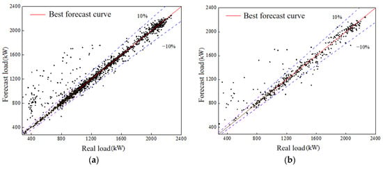
Figure 1.
Load-forecasting results without PCA dimensionality reduction. (a) Training set prediction results; (b) test set prediction results.
In the training set forecasting results, when the air conditioning system load is within 1200 and 2400 kW, the error between the load-forecasting results and the real value is basically within ±10%, and the load-forecasting accuracy is high; when the load of the air conditioning system is within 280 and 1200 kW, the predicted value of some data is far greater than the real value. In the test set’s forecasting results, it can be found that the error between most load-forecasting results and the real value is within ±10%. The absolute errors of the prediction results of the training set and the test set are counted. The data with an absolute error of less than 10% account for 92.22% and 88.27%, respectively, and the data with an absolute error of less than 20% account for 94.06% and 92.92%, respectively. The load-forecasting results have high accuracy.
In the load-forecasting results after dimensionality reduction in input parameters, the optimization results of core parameters c and G are 4 and 1.414, T = 256.74 s. RMSE = 169.72, R2 = 0.8843 for the prediction results of the training set, RMSE = 180.33, R2 = 0.8630 for the prediction results of the test set. The prediction results of the test set and the training set are similar, and the generalization performance of the model is good. The load-forecasting results of the training set and test set are shown in Figure 2.
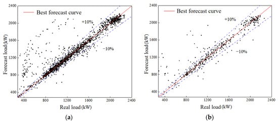
Figure 2.
Load-forecasting results after dimension reduction by PCA. (a) Training set prediction results; (b) test set prediction results.
Compared with the load-forecasting results without dimensionality reduction in input parameters, the accuracy of load forecasting after dimensionality reduction is significantly reduced. Among them, the RMSE of the training set is increased by 43.66%, R2 is reduced by 6.6%, the RMSE of the test set is increased by 37.77%, and R2 is reduced by 7.1%, but the modeling process time is reduced by 41.06%. In conclusion, using PCA to reduce the dimension of input parameters can avoid the increase in the model calculation cost caused by too many input parameters, but it will reduce the accuracy of load forecasting, which may be due to the loss of information when extracting principal components from high-dimensionality data.
The actual load-forecasting results show that when PCA is not used for data dimensionality reduction, T = 435.59 s, RMSE = 118.14, R2 = 0.9468, RMSE = 130.89, and R2 = 0.9289; after data dimensionality reduction with PCA, T = 256.74 s, RMSE = 169.72, and R2 = 0.8843 for the prediction results of training set, and RMSE = 180.33 and R2 = 0.8630 for the prediction results of the test set. Therefore, whether PCA is used for dimensionality reduction or not, the prediction results of the test set and training set are similar, which shows that the model has good generalization performance; that is, the operation-load-forecasting method of an air conditioning system based on data mining proposed in this paper is feasible.
3.2. Analysis of Water System Operation Optimization Results
- (1)
- Optimal operation control strategy of a groundwater system with different load rates
The actual operating parameters of the system under different load rates are obtained from the data derived from the energy management system. Based on the load-forecasting results, the operating parameters of water system equipment are optimized. The results are shown in Table 3.
Table 3.
Water system optimization parameters of water chiller under different loads.
It can be seen in Table 3 that within the range of a 25~90% load rate, the relative error of load-forecasting results is within ±10%. The actual total load of 14 working conditions in the table is 22,761.8 kW, the predicted total load is 22,913.2 kW, and the relative error is 0.64%. The load-forecasting effect is good. In terms of equipment operation parameters, with the increase in load rate, the outlet temperature of chilled water decreases from 12.00 °C to 9.30 °C. When the load rate is below 80%, one cooling water pump and cooling tower can meet the load demand, and when the load rate is above 80%, two can meet the load demand. The start and stop of the cooling tower fan are interlocked with the cooling water pump; one set of chilled water pumps can meet the load demand when it is operated at a 25% load rate, and two sets can meet the load demand under other working conditions.
- (2)
- Energy consumption analysis of the water system
It can be seen in Table 3 that the optimization strategy has a certain energy-saving effect in the range of a 25%~90% load rate, and the energy-saving effects of the optimization strategy are different under different load rates. When the load rate is 25.4%, the system energy-saving rate is the highest, which is 29.45%. When the load rate is 80.37%, the system energy-saving rate is the lowest, which is 0.43%. The average energy-saving rate of the optimization strategy under different load rates is 12.40%.
4. Conclusions
This paper takes the central air conditioning system of a hotel as the research object, establishes the load-forecasting model based on SVR through MATLAB, and establishes the equipment energy consumption model based on the principle of each piece of equipment in the water system. On this basis, the objective function of energy consumption optimization of the hotel’s water system is established, and the dynamic optimization of operating parameters of the water system at different load rates is realized. The main conclusions are as follows:
- (1)
- The air conditioning load-forecasting model based on the SVR principle has similar prediction results in the test set and the training set, indicating that the model generalization performance is good. Moreover, whether PCA is used for dimensionality reduction or not, the load-forecasting model has good generalization performance. The advantage of PCA is that it can significantly reduce the calculation cost of the SVR model, but it reduces the accuracy of load forecasting. The reason for this may be the information loss caused by extracting principal components from high-dimensionality data.
- (2)
- Based on each equipment model of the water system, the objective function of energy consumption optimization of the water system is established. The operating conditions of each piece of equipment and the energy conservation of the heat-exchange process are taken as the constraint conditions, and the predicted air conditioning load is taken as the disturbance variable. SQP is used to solve the energy consumption optimization problem of the hotel air conditioning water system with controllable variables and disturbance variables and realize the optimization of operating parameters of sewage system at different load rates. After optimization, the average energy-saving rate of the water system with different load rates is 12.40%, which shows that the water system optimization based on load forecasting proposed in this paper has a good energy-saving effect.
Author Contributions
Data curation, K.W. and X.C.; Investigation, K.W. and B.Z.; Writing—original draft, X.C.; Writing—review & editing, Z.H. All authors have read and agreed to the published version of the manuscript.
Funding
This study was funded by National Natural Science Foundation of China (no. 51608001), and Anhui Province Undergraduate Innovation and Entrepreneurship Training Program (no. S202010360231).
Institutional Review Board Statement
Not applicable.
Informed Consent Statement
Not applicable.
Data Availability Statement
Not applicable.
Conflicts of Interest
The authors declare no conflict of interest. The funders had no role in the design of the study, in the collection, analyses, or interpretation of data; in the writing of the manuscript, or in the decision to publish the results.
References
- Huang, Z.; Gan, L.; Jiang, L.; Shen, Z. Study on the current situation of energy consumption and energy quota of public buildings in Maanshan. Build. Energy Effic. 2020, 48, 125–127, 138. [Google Scholar]
- Zhang, T.; Lu, Y.; Huang, Z.; Hiroshi, Y. Analysis of the composition of CO2 emissions in residential buildings during the use phase. HVAC 2012, 42, 106–109. [Google Scholar]
- Zhang, Z.; Li, Y.; Zhang, Y.; Wu, X.; Di, H.; Zhang, X. Research and analysis on energy consumption of existing public buildings in hot summer and warm winter areas. Build. Energy Effic. 2020, 48, 11–15. [Google Scholar]
- Ding, X.; Hu, C.; Liu, X.; Sun, L. Research on energy consumption of typical high star hotel buildings in southern Jiangsu and analysis of energy saving potential. Jiangsu Archit. 2020, S1, 90–93. [Google Scholar]
- Li, Y.; O’Neill, Z.; Zhang, L.; Chen, Z.; Im, P.; Degraw, J. Grey-box modeling and application for building energy simulations—A critical review. Renew. Sustain. Energy Rev. 2021, 146, 111174. [Google Scholar] [CrossRef]
- Deb, C.; Schlueter, A. Review of data-driven energy modelling techniques for building retrofit. Renew. Sustain. Energy Rev. 2021, 144, 110990. [Google Scholar] [CrossRef]
- Cui, Z.; Cao, Y.; Wei, J.; Mao, X.; Li, R.; Tang, Y. Progress of research application of data mining technology in the field of building HVAC. Build. Sci. 2018, 34, 85–97. [Google Scholar]
- Yan, C.C.; Wang, S.W.; Xiao, F.; Gao, D. A multi-level energy performance diagnosis method for energy information poor buildings. Energy 2015, 83, 189–203. [Google Scholar] [CrossRef]
- Liang, Z.; Wu, J.; Xie, Z. Identification of actual operation patterns of variable frequency air conditioners and data mining. J. Mech. Eng. 2019, 55, 194–202. [Google Scholar]
- Zheng, Z.X.; Li, J.Q.; Duan, P.Y. Optimal chiller loading by improved artificial fish swarm algorithm for energy saving. Math. Comput. Simul. 2018, 155, 227–243. [Google Scholar] [CrossRef]
- Wang, T. Study on Optimization of Chiller Plant and Chilled Water Pump Operation Based on Real Measurement. Master’s Thesis, Dalian University of Technology, Dalian, China, 2017. [Google Scholar]
- Cheng, R.; Yu, J.; Zhang, M.; Feng, C.; Zhang, W. Short-term hybrid forecasting model of ice storage air-conditioning based on improved SVR. J. Build. Eng. 2022, 50, 104194. [Google Scholar] [CrossRef]
- Feng, C.; Li, Q.; Wang, G.; Li, H. Hourly load forecasting of nZEB in severe cold area based on dest simulation and gs-svr algorithm. J. Shenyang Archit. Univ. (Nat. Sci. Ed.) 2022, 38, 149–155. [Google Scholar]
- Zhou, X.; Zi, X.; Liang, L.; Fan, Z.; Yan, J.; Pan, D. Forecasting performance comparison of two hybrid machine learning models for cooling load of a large-scale commercial building. J. Build. Eng. 2019, 21, 64–73. [Google Scholar]
- Wei, D.; Jiao, H.; Feng, H. Nonlinear Predictive Control of Freezing Station System Based on Load Prediction. Control. Theory Appl. 2021, 1–12. Available online: http://kns.cnki.net/kcms/detail/44.1240.TP.20210311.1555.032.html (accessed on 12 August 2021).
- Li, Z.; Li, C.; Zhu, H. Parameter optimization research based on SVR air conditioning load prediction model. Build. Energy Conserv. 2021, 49, 43–48. (In English) [Google Scholar]
- Luo, X.; Chen, H.; Lu, X.; Xiong, Y. SVM mill load prediction based on grid search and cross-validation. China Test. 2017, 43, 132–135, 144. [Google Scholar]
- Liu, G.; Liu, Z.; Yan, J.; Zhou, X. Research on operational characteristics analysis and energy-saving optimized operation method of centralized air-conditioning chilled water system. Build. Sci. 2018, 34, 127–140. [Google Scholar]
Publisher’s Note: MDPI stays neutral with regard to jurisdictional claims in published maps and institutional affiliations. |
© 2022 by the authors. Licensee MDPI, Basel, Switzerland. This article is an open access article distributed under the terms and conditions of the Creative Commons Attribution (CC BY) license (https://creativecommons.org/licenses/by/4.0/).