Abstract
The continuous change process in the impact of differences in public transport accessibility has not been explained specifically in previous studies. This study reveals that the interaction between two continuous explanatory variables has a significant impact on the explained variable in the hedonic model. The study takes the accessibility variable in the house price model as an instance, dividing the accessibility variable of the residential community into two parts. The first part is the rail accessibility defined by the Euclidean distance from the residential community to the nearest rail transportation station. The second part is the road accessibility defined by two Space Syntax indicators, connectivity and carrying capacity, according to the spatial pattern of the road network. As demonstrated by the spatial interactive regression model, this research finds that road connectivity has a significant regulating effect on the impact of the distance to the closest rail station on house prices based on the empirical evidence from Fuzhou, China.
1. Introduction
The discussion of housing is an unavoidable topic of human development. Among the many topics in the discussion of housing, exploring the direction of house prices has always been a key component. In order to allow people more reasonable living costs, and under the premise of sustainable income control, finding suitable living conditions for their own needs has become an important reason for ordinary people to discuss house prices [1]. The government also pays attention to the issue of housing prices in order to balance the interests of different parts of the city through the location selection of public facilities, so as to maintain social harmony in a long-term sustainable manner [2]. Simultaneously, researchers hope to use house prices as a reference standard to measure the value of space so as to conduct long-term exploration of variables that affect it, which allows them to maintain a high enthusiasm for the issue of property prices [3]. Consequently, in essence, the reason why different groups pay attention to property prices is to maintain a high-quality living environment in a long-term sustainable manner.
There are many variables that affect housing prices. Whether it is a variable factor that has been confirmed or one that has not, the research will continue to be refined and expanded over time. Furthermore, different variables have not only a single linear relationship to the impact of house prices, but also due to overlapping or mutually exclusive functions between different variables so that there is a moderating effect between them. Thus, it is very important to explore the variables that affect house prices and the interactive moderating effects between variables.
Due to the accessibility attribute having a significant impact on the value of the property, the impact of accessibility variables on house prices has been a hot research direction for a long time [4]. Among research documenting in the impact of accessibility variables on house prices, rail accessibility and road accessibility are two main factors which define accessibility. Therefore, this study will take rail accessibility and road accessibility as examples to reveal the mutual moderating relationship between the two variables on the impact of house prices.
Scholars explore how property prices are affected by these accessibility variables respectively from familiar angles. These angles often need to be able to specifically reflect the characteristics and accuracy of residential objects. When analyzing impact of subway accessibility variables on property price, most previous studies reveal the influence scope and extent of subway accessibility variables on property prices by calculating the Euclidean distance between rail stations or road travel distance. To be specific, Ronghui Tan et al., (2019) researched subway traffic in Wuhan, finding that ordinary rail stations affected the price of surrounding properties within 1600 m, while transfer stations influenced that within 4800 m [5]. Moreover, Elif Can Cengiz et al., (2019) pointed out that the price of properties was higher near subway station facilities than those in the distance [6]. Since the road’s spatial pattern is very decisive for road accessibility, the quantitative evaluation of the spatial pattern form can deeply reflect the degree of road accessibility. Thus, in terms of research on the impact of road accessibility on property prices, researchers focus on the influence of characteristics of road network forms. In this regard, Law (2017) investigated London and drew a conclusion that property price was significantly affected by the perception of difference in road network forms, and the influence became stronger over time [7]. Another example is Liang, who proved through empirical evidence in Victoria, Australia that the removal of urban level crossings changed traffic connectivity and road accessibility, resulting in an impact on housing prices [8]. However, the increase in traffic connectivity and road accessibility emphasized in Liang’s research is a local judgment based on human intuition, rather than a geometric evaluation based on the overall urban road network. Therefore, the study will be carried out based on the explanatory variables with reference to the rail accessibility reflected by the Euclidean distance between the residence and the rail station and the road accessibility reflected by the road spatial pattern of the road network where the residence is located.
Among the existing literature, when discussing the impact of two or more explanatory variables on house prices due to their interactions, scholars mainly compare the difference in interactions by building a regression model in groups or adding dummy variable items. However, it is impossible to accurately assess regulatory effects of continuous variables. Specifically, Jen-Jia Lin et al. modeled data by groups of properties along Metro Taipei Redline before the opening (1993–1995) and after the opening (1997–1999), in order to reveal the impact of the Taipei Rapid Transit System on house prices before and after the opening [9]. Although the impact was different, the continuous change process of this difference could not be explained.
In general, it is of great value to adopt interaction items in econometrics to analyze how explained variables are affected by interaction of multiple non-colinear continuous explanatory variables. As mentioned in the beginning, urban transportation mainly includes subway and roads whose construction helped to improve the carrying capacity of the urban transportation system and drive the regional economy [10]. At the same time, houses or properties are a key component of urban areas. Therefore, it is significant to study urban development via revealing the impact of subway accessibility and road accessibility on house prices by the interaction principle. As for urban residents, they pay great attention to availability when purchasing houses. They want to know the direct impact of subway accessibility and road accessibility, but are eager to figure out the regulatory effect of interactions on house prices, so as to select the best house locations in accordance with economic strength and transportation demand preferences.
Therefore, this study introduced the concept of interaction into the hedonic price model, and established linear interactive regression models and a spatial interactive regression model for analyzing non-collinear continuous explanatory variables, so as to explain the mutual regulatory effects of the subway traffic accessibility variable and road accessibility variables on house prices. It is hoped that this will provide a valuable reference for government transportation construction, buyers purchasing properties and literature references of scholars. Due to the construction of urban transport, there is a significant increase in the value of urban land [11]. Therefore, by studying the differences in land value enhancement, it is possible to help the government to issue targeted land fiscal policies [12]. These land finance policies can help the government to obtain effective financing compensation for transportation construction, so as to continue to promote urban development and balance the development level of the region [13]. For individual home buyers, in addition to directly obtaining the reference for their own living choices, they can also obtain advice for their own investment in real estate, so as to obtain the maximum land investment income. For scholars, capturing these differences in land value improvement can better improve the theoretical system of spatial economics and establish more diverse disciplines, such as economics, planning, geography, sociology and so on.
The remaining research content falls into four sections. Section 2 presents a literature review for the research basis. Section 3 discusses the research framework, data sources and process. In Section 4 the research results obtained are presented. Section 5 provides discussions of the findings and of limitations based on the data results, and concludes with the implications of the study.
2. Literature Review
After the introduction of the research background, this study will review the literature discussing the application of the hedonic price model to study influences on house prices, interactive models of house prices in the past, the impact of the distance of subway stations as well as road network forms.
It is a very common method to study house prices through hedonic price models. Hedonic price model is a research method that decomposes the value composition of an item, and constitutes an item model by establishing the values of multiple features to evaluate the total price of the item. It was composed of consumer theory proposed by American scholar Lancaster in 1966 and the supply–demand equilibrium model by American economist Rosen. The earliest hedonic price model was often used to analyze price composition of commodities such as vegetables and automobiles [14]. It was not widely applied in the analysis and research of house prices until Ridker et al. [15] first studied the impact of the improvement of environmental quality on house prices through the model. Most researchers divided it into characteristic variables, a neighborhood characteristic variable and a location accessibility characteristic variable [16]. As a recent example, Cui et al. [17] used the hedonic price model to demonstrate that different types of consumers have different demand preferences for housing. Zou et al. [18] demonstrate the impact of environmental quality on housing rents. Claudia Hitaja et al. [19] and Wang and Lee [20] through their studies on cities in the United States and China, respectively, proved that air quality levels also have a real impact on housing prices. Sumit Agarwal et al. [21] in Singapore confirmed the impact of school districts on housing prices. In addition, the hedonic price model will also be applied to the analysis of other living environments, which will also indirectly affect the regional impact on housing prices. For instance, Sumit Agarwal and Koo Kang Mo. [22] analyzed periodic congestion charging in the context of Singapore, which concerned the impact of rate adjustments on changes in commuters’ mode of transportation choices.
In the process of researching housing prices by previous scholars, interaction models have been used to study housing prices. In the traditional general hedonic price model, it is mainly used to investigate the influence of non-collinear explanatory variables on explained variables, while the interactive regression model serves for the influence of correlation of multiple variables with explained variables. However, in the past, the interaction item model was frequently adopted to explore the impact of interaction between non-continuous dummy variables on explained variables, while an interactive regression model defined by continuous variables was relatively rare. To be specific, Ting Xu [23] introduced an interactive model of dummy variables defined by environmental location and household classification, to prove that the marginal price of housing attributes in Shenzhen varied with the absolute location environment and household condition rather than being invariable. Similarly, Janet Currie et al. [24] defined the opening status of factories and explored whether properties were affected by the factory through dummy variables. It was found that prices of properties within 0.5 km of factories emitting toxic gases declined by appropriately 11%. Meanwhile, concerning the distance of properties from new subway stations and house transaction time, Junhong Im and Sung Hyo Hong [25] grouped property transaction data in Daegu, South Korea, to compare the premium of house prices by new subway stations under the influence of old subway stations. They classified the distance between properties and the new subway station and time difference before and after the announcement of new subway station policy into dummy variables, and then established an interactive regression model. Finally, a conclusion was drawn that a residence price premium was obvious for properties within 500 m of new subway stations and 5000 m away from original subway stations.
The impact of rail stations on house prices has been a hot research topic in recent decades. As a major form of infrastructure, urban subway stations have produced a significant impact on firm location, employment and population growth. This has been demonstrated by Mayer, T. and Trevien, C. [26] through empirical evidence in Paris. Similarly, the impact on house prices is also quite significant. Regarding this, Zheng Jiefen and Liu Hongyu [27] examined and analyzed data of Shenzhen subway, realizing that prices of properties within a 400m to 600m radius of subway stations were higher. With the change in distance from subway stations, price rising was dramatically different. Xinyue Zhang and Jiang Yanqing [28] researched data of second-hand houses within 6 km of Nanjing Metro Line 1 and Line 2, and verified that when the distance was less than 500 m, house price rose highest, and rising was still obvious within 2 km. With distances greater than 2 km, this influence was negligible. Similarly, Almosaind et al. [29] analyzed house price data around Portland’s subway transit stations to find that price of properties within 500 m of subway transit stations soared by 10.6%. Haizhen Wen et al. [30] studied house price data along Hangzhou subway stations and concluded that house prices were negatively correlated with the distance to subway stations; that is, for every 1% decrease in distance, prices would rise by 0.049%. As the distance increased, the value-added effect was weaker. More precisely, properties within 500 m had the highest premium (6.2%). While the distance was over 1500 m, the value-added rate dropped sharply (2.1%). Armstrong and Rodriguez [31], through a study of 1860 residential samples in Massachusetts, USA, proved that the premium capacity of rail stations for residences is not the same outside the half-mile buffer zone of rail stations. In addition, differences in distance and degree of house prices affected by subway stations would also change with variation in other external conditions. Having analyzed the transaction prices of 722 residential communities near Shenzhen subway stations, Yang et al. [32] discovered that the price of surrounding properties was positively affected by rail accessibility (1200 m in urban area and 1600 m in the suburbs). The influence became weaker with properties more distant from the urban subway station.
Previous scholars have also tried to study the impact of road network morphology on house prices. Traditional road traffic accounts for the largest proportion in urban traffic systems. It is one major way for people to travel, so it affects house prices greatly. Many scholars have conducted studies in this regard. However, due to the display complexity of roads on a three-dimensional level, they are usually quantized from a two-dimensional plan. Relevant research began earlier in Western countries; for instance, Matthews et al. [33] conducted an empirical study of Seattle, finding that house price was affected by the road network form variable when at a walking scale of about 500 m. Xiao et al. [34] concluded that improvement of road network accessibility improved prices. Moreover, taking Shanghai as a case, Yao Shen and Kayvan Karimi [35] explained how house prices in different areas were influenced by road network centrality and functional connectivity based on traditional spatial syntactic analysis. In China, the research on relationship between road network form and house price was still in its infancy. The hedonic price model was introduced by Xiao Yang et al. [36] to study Nanjing, and a conclusion was drawn that road network structure produced two economic effects on house prices in the downtown area. In addition, Yang Ying et al. [37] analyzed geographic weighted regression (GWR) and realized that the house price of second-hand houses was significantly affected by road network forms in Chengnan and Chengbei Districts of Xi’an City. Based on the sDNA model, Gu Hengyu et al. [38] discussed the influences of road network forms, and summarized that house price was impacted differently due to different description methods of road network forms.
3. Methods
This study was based on the idea of “hypothesis validation”. Through the collected data, a spatial regression interaction model was established to explore the significance of the interaction terms of the target variables, so as to give relevant research results. Finally, the study ensured the stability of the results through Robustness checks.
3.1. Research Framework
According to the literature review, the study proposed the research hypothesis that “road network forms play different roles in regulating the extent of the influence of distance to subway stations on house prices, and vice versa”. Based on the hypothesis, this research process includes five steps (Figure 1). The first step is road network spatial data reflecting the realities of roads, and the spatial syntax analysis method is applied to quantitatively collect urban road accessibility and other variables impacting house prices. In the second step, on the basis of the collected explanatory variables of properties, a hedonic price regression model is applied; interaction of accessibility variables was used to construct a linear regression interaction model for house prices. According to the linear interactive regression model, the third step deduces generality of space, and considers spatial auto-correlation of explained variable (house price) and spatial nuisance of error to build a spatial interactive regression model. The fourth step was to perform a robustness test of the spatial regression interaction model. The last step was to analyze and summarize based on the model regression coefficients obtained above.
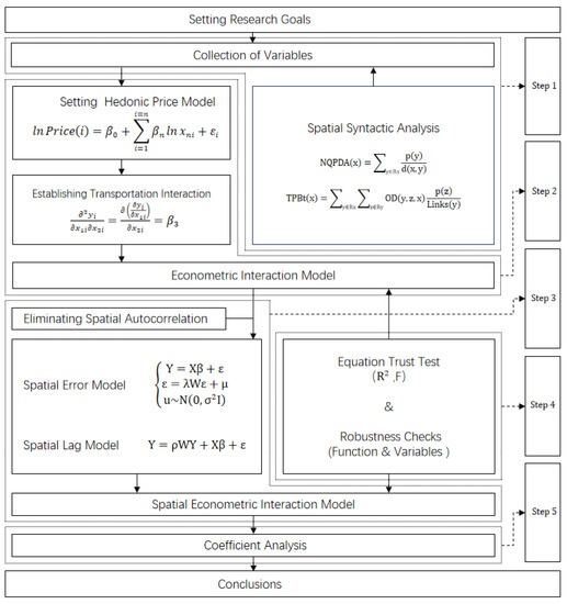
Figure 1.
Frame diagram.
The above research process can be applied to the variable interaction research of the hedonic price model of house price, no matter whether the variable is a continuous variable or a dummy variable. This is a further attempt compared to previous scholars who only used dummy variables to establish interaction models when they introduced interaction variables to discuss the impact of house prices.
On the other hand, the research process also has some limitations. One of the limitations of this research process is that the third step model of the research is based on spatial auto-correlation theory, which uses cross-sectional spatial data for spatial analysis, which fails to take temporal variables into account. In addition, there are other specific limitations of the study, which will be discussed in detail in the final chapter of the paper.
3.2. Methodology
3.2.1. Space Syntax Analysis
After establishing the research framework, this study adopted space syntax to calculate two sets of data of road accessibility—closeness, reflecting road connectivity, and betweenness, representing road carrying capacity [39]. According to space syntax theory, the definition of space was understood from scale and space levels, and it helped to further analyze the complex relationship between scale and space. In this study, mainly road space was analyzed.
Calculation of closeness means the efficiency and convenience of a certain road segment to search for other roads to be reached within search radius R. In the study, the value is represented by NQPDA (Network Quantity Penalized for Distance Analysis). The global closeness (NQPDAn, abbreviated as NQ) is that search radius R value is closeness value of the whole research scope. NQ shall be used to indicate the first measurement indicator of road segment in road accessibility (connectivity). In order to make the expression process simple, this study abbreviated the concept of NQ as closeness, with a calculation parameter model as follows:
wherein, NQPDA(x) represents closeness; p(y) means relative importance of index of node y in overall data evaluation within the range of search radius R; d(x,y) means the shortest topological path between node x and node y; Rx is the area with x as the center and R as radius.
Betweenness can be understood as the passing probability of traffic passing from one point to another of the road section within search radius R; it will be represented by TPBt (abbreviated to TP, the sum of geodesics that pass through the link from one point to another). Therefore, in the spatial syntax analysis model, the higher the value of betweenness, the greater the possible traffic volume carried by the road, and vice versa. In the spatial syntax line segment model, betweenness describes road carrying capacity in urban traffic, and is used in analysis of traffic flow and traffic evacuation capacity. This is the second measurement indicator to describe road accessibility. In addition, for easy expression, the global travel degree used in the study is referred to as betweenness in the following process, with calculation parameter model as below:
wherein, TPBt(x) represents betweenness of the model; OD(y,z,x) means the shortest topological path from node y to node z through road section x within range of search radius R.
3.2.2. Linear Regression Model (OLS)
Hedonic Price Model (Hedonic)
The hedonic price model is a linear model function widely used in land value, price evaluation and prediction in real estate and other fields [40]. The specific function models include linear, semi-logarithmic, and dual logarithmic forms. However, the dual logarithmic model could more effectively reveal significant marginal utility of transaction price on house characteristics during purchase, so the simulation process was more practical and reasonable. Accordingly, the hedonic model used in this study consulted a dual logarithmic model [41] commonly used by previous scholars. The relationship between house price and each explanatory variable is listed as follows:
Among them, Price in Price(i) represents house price, i means data in the i-th real estate, and Price(i) represents average price per square meter of the i real estate, including the sum of the price of the house itself and renovation costs; that is, the average transaction price of the i real estate. The n in xni is a characteristic factor, which represents the n-th characteristic influencing factor among many attributes; i indicates data in the i-th real estate, and xni is data performance of the n-th characteristic influencing factor in the i-th real estate. βn is the non-standardized coefficient of the n-th relevant characteristic-influencing factor on house price; εi is a stochastic error term. In addition to the coefficients in the model, regression analysis also exposes strong or weak significance of major positive or negative explanatory variables that affect house prices.
Interactive Regression Model
In econometrics, when linear regression model is added with an interaction term, it becomes a regression equation model with special processing form. The interaction is the result of mutual effect of two or more influencing factors. To some extent, this method broadens interpretation angle and depth of explained variables being affected by different explanatory variables in the regression model. During research, additive interaction terms and multiplicative interaction terms were considered separately. However, after comparison of the significance of relevant data, a multiplicative interaction model with better fit and significance was selected as the research method for interaction. The specific calculation formula model is as follows:
Find the partial derivative of xmi for the first function to obtain second function formula above. In other words, after an interaction term is added to the original model, marginal effects of explanatory variables xmi and yi change; marginal effects originally depended on constants changing into that relying on explanatory variable xni; that is, the linear function equation model associated with xni. When βmn > 0, the marginal effect of xmi and yi will increase as the variable xni increases. This change is called “synergy effect” in the marketing. On the contrary, when βmn < 0, the marginal effect of xmi will decrease with the rising of xni. Continuously find the partial derivative of xmi for the second function to obtain third function formula above. βmn is the “interaction effect” in the interaction model, which is specifically expressed as the relative effect of an explanatory variable on yi and strength of the effect affected by another explanatory variable.
3.2.3. Spatial Regression Model
Spatial Error Model
The spatial error model specifically describes the influence of spatial nuisance dependence on explanatory variables in the space as a whole. Alternatively, it can be understood that a certain spatial disturbance will affect other spaces along with space benefits. The spatial error model is suitable to explain that spatial disturbance occurring in a certain space between regions will be transmitted to e adjacent space in the form of covariance, which is the result of random interaction in space. These effects are long-term and continuous, and will gradually decay with time or space factors. The calculation model is as follows:
wherein, λ represents spatial error correlation coefficient in spatial error model; W means spatial weight matrix with multiple spatial data points in spatial error model, which explains proximity relation of explanatory variables; and wij describes the correlation between individual error terms of the j-th and the i-th spatial data point.
Spatial Auto Regression Model
The space lag model means that a certain space is not only affected by the explanatory variables of the space, but also other similar spaces in the space. It aims to analyze the impact of spatial auto-correlation of house prices on house price itself. The spatial auto regression model is as follows:
Among them, in the spatial lag model, Y is a matrix of explained variables; ρ represents the spatial effect coefficient; X means a matrix of explanatory variables; β represents vector of parameters. Similarly, W is a spatial matrix with multiple spatial data points; that is, to describe the mutual influence relationship between explanatory variables and the adjacent spatial explanatory variables. The n in the matrix means n spatial data points, and the matrix explains proximity relation of spatial regions between spatial data points. The spatial data points in each row represent a relationship set between a spatial unit and its proximity space, such as W11~W1n, indicating spatial proximity relation between spatial data point 1 and spatial data points 1, 2, …, n.
3.3. Data
This study mainly selected 1245 residential community samples from twelve county-level administrative regions under Fuzhou City, Fujian Province, China as the research object (Figure 2). In previous studies on house prices, Fuzhou was rarely used as a reference city due to its low international reputation. However, in recent years, Fuzhou has been in the development stage of urban rail construction, so it is quite meaningful to study the impact of rail station on house prices. Furthermore, the study results can guide and review the urban rail station under construction. Therefore, comprehensively considering the novelty and value of the research target, the study selected Fuzhou as the reference city.
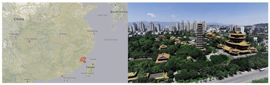
Figure 2.
Location and Perspective of Fuzhou City.
The data were all spatial market data from March 2021 in this study, and the dependent variable house price data are the average data in one month. Since other variables basically did not change within a month, the spatial cross-section data on 15 March 2021 are used as a representative. The selection of independent variables is the result of significant screening based on the experience of literature which may affect house prices. Average price was taken as basic unit of comparison, and large real estates with different residential properties were eliminated (such as villa estates), in order to avoid abnormal fluctuation of price of each house due to exquisite degree of decoration, north/south orientation, and elevator equipment, as well as other individualized and diversified factors [42].
Considering the realities of the study area, a brief introduction to the variables of the study is now carried out. The explained variable was represented by the average transaction price of residential communities, and information and data related to residential community were used as the explanatory variables that were divided into three categories: (1) self-characteristic information data and location information data, which covered the administrative area factor, urban location factor, nature of property rights, construction years, types of floors, plot ratio, greening rate, the level of property management fees, and educational resources (whether there were key primary and secondary schools) of residential communities. Since in Fuzhou, there are only the Second Ring Road and the Third Ring Road in the urban area, and there is no First Ring Road, the entire urban space area is divided into three areas: the area within the Second Ring Road, the area from the Second Ring Road to the Third Ring Road, and the area outside the Third Ring Road. Among the variables, we used dummy variable 1 (CityLC1) and dummy variable 2 (CityLC2) of the urban space area to distinguish the three regions geographically. For the distinction of administrative space regions, we used the dummy variable (AdmRC) of whether it belongs to the city administrative region as the criterion. (2) Other external neighborhood explanatory variables included explanatory variables positively correlated with prices, such as shopping malls, grade 3 and first-class hospitals, scenic spots, green spaces, and important water bodies, and those negatively related to prices, namely funeral facilities, factories, gas stations and garbage dumps. Their influence on properties rested with the distance from residential communities. (3) The accessibility explanatory variables contained road accessibility variables (closeness, betweenness), rail accessibility variable (Euclidean distance to the closet subway station), and interaction variables between road accessibility variables and rail accessibility variables. Note: The price data comes from Anjuke official website database, and Ovital Map provides neighborhood and accessibility data. Please refer to figures below for specific explanatory variable details (Table 1, Figure 3) and road calculation results (Table 2, Figure 4 and Figure 5).

Table 1.
Descriptive statistics of the property dataset (N = 1245).
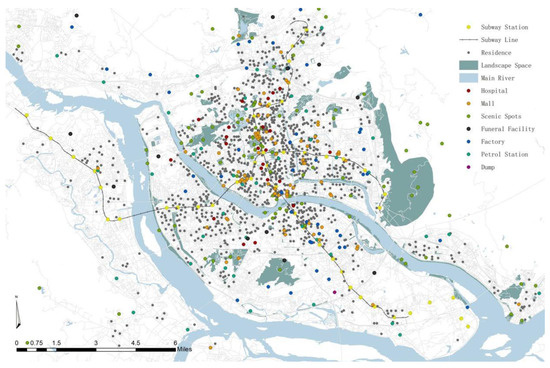
Figure 3.
Schematic of the spatial distribution of variables.
Table 2.
Statistics of the Space Syntax Analysis (N Roads = 56,228, N Residences = 1245).
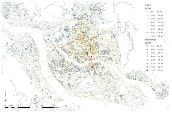
Figure 4.
Result of connectivity.
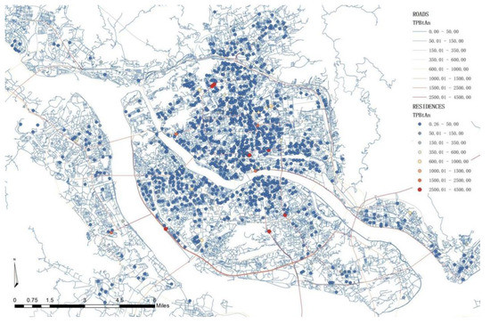
Figure 5.
Result of carrying capacity.
4. Results
4.1. OLS Regression
After sorting out collected explanatory variables of the residential community, this study obtained a hedonic price model through regression, and then added interaction terms of road description variables and a rail distance variable for another linear regression of the model, acquiring a linear interactive regression model of house prices.
According to the regression equation of the interactive model, regression was generally good (R2 ≥ 0.675), and had the expected explanatory power.
From the perspective of significance, house price was significantly affected by explanatory variables (distance to subway stations, road network proximity), and the interaction of both. However, and the influence of road network betweenness and its interaction with distance to subway stations was insignificant.
The significant characteristics expressed by other control variables are as follows. Variables (locations in urban area, in second ring road and in the third ring road, average property fees, key primary schools and key middle schools nearby, distance to grade 3 and first-class hospital, distance to funeral facilities, distance to factories, distance to important water bodies and the distance to garbage disposal facility) exerted a significant impact on house prices. The impact of distance between residential communities and scenic spots on house price was generally correlated. However, the relationship between house prices with explanatory variables (nature of properties, building year, types of floors, greening rate, plot ratio, the distance to green space, distance to the closet business district, and the distance to the closet gas station) was insignificant.
This study conducted two robustness check analyses so as to verify the variables of distance to subway station, road network proximity, and the stability of the significance of their interaction. In the first check, some variables with low significance were removed and then regression fitting was performed again. In the second check, the natural logarithm of the road accessibility variable in the model was replaced by a constant, and a regression test was obtained similar to the previous regression, proving the reliability of above linear regression results. Please refer to Table 3 for overall results of the linear regression model and the test model.
Table 3.
Regression results of the OLS.
4.2. Interactive Spatial Effect on Property Prices
Based on the linear interactive regression model established above, this study further took into account spatial errors in and spatial correlation factors of explained variables respectively into the model. In accordance with the spatial location distance of properties, a geographic spatial matrix was established to construct a spatial interactive regression model.
After consideration of the spatial correlation of errors and the spatial autocorrelation of explained variables, the spatial interactive regression model constructed had a slightly better regression fitting degree than the linear regression interaction model . More importantly, significance and coefficient characteristics of interaction terms were consistent with those in the linear interactive regression model. This indicated impact of interaction between distance to subway stations and road network proximity on property in the linear model was also suitable for spatial relationship. The influence would not become weak with the changes in the relative spatial location of properties.
Similarly, for the purpose of testing stability of calculation data, it examined robustness of the spatial mode through two steps. The first was the change in the functional form of the fitting model. The previous dual-logarithmic model was replaced with a semi-logarithmic model that took the natural logarithm of the explained variable and the original value of the explanatory variable for regression fitting of the spatial model. Second was the reduction in the number of explanatory variables. Explanatory variables insignificant in the previous regression were removed and spatial linear regression analysis was conducted. Next, on the basis of the first test, dummy variables in all explanatory variables were abandoned again for another spatial regression analysis. After the test regression model was obtained, this study compared coefficient significance and characteristics of the tested spatial regression equation and the original spatial regression equation, and confirmed that the research results of the spatial interactive regression model were reliable. In Table 4 and Table 5 results of the spatial regression model and robustness test are listed.
Table 4.
Regression results and Robustness checks of the SLM and SEM.
Table 5.
Robustness checks results of the SLM and SEM.
After the spatial regression interaction equation was acquired, functional images were used to represent the impact of interaction on house price in different regions in order to reveal the impact of interaction on explained variables in different spatial regions (heterogeneous regions). According to the administrative districts of residential communities, data of existing properties were divided into five sub-sets (Gulou District, Taijiang District, Cangshan District, Jin’an District, Minhou County) along the existing subway lines. The spatial classification was shown in Figure 6. In functional images, sample residential communities in Fuzhou were based on the average level of all 1245 samples, and variable values of sample residential communities were subject to an average level in the administrative districts (continuous variables take the average value in the area, and dummy variables are determined as 0 or 1 by rounding the average value; see Table 6). As the value method of control variables, specific function images of each area sample are shown in Figure 7.
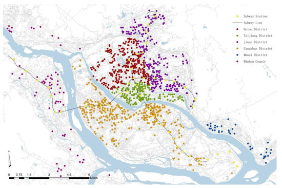
Figure 6.
Administrative Division of Residential Space.
Table 6.
Mean Statistics of Sample Properties (N = 1245).
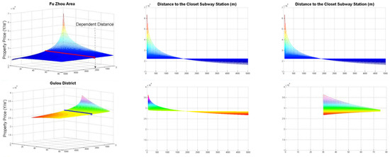
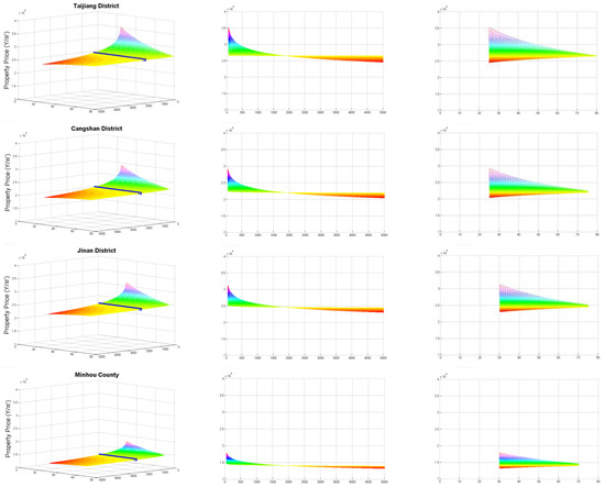
Figure 7.
The impact of accessible variables on property price.
5. Discussions and Conclusions
5.1. Discussions of Findings
Findings of the analysis are drawn as per the above data table and coefficient interpretation analysis of images:
- (1)
- This study classified the explanatory variables of properties and evaluated their significance, positive and negative effects. Among them, there was a significant negative correlation between the distance to subway stations and house price, or in other words, subway transportation produced a significant impact on house price. Traditional research showed that house price was strongly positively affected by house advantage factors such as the regional administrative nature, urban centrality, greening rate, property service level, key elementary and middle school districts, convenience of hospitals, and convenience to access water in the landscape. Apart from that, NIMBY factors (distance to funeral service sites, factories, and garbage dumps) produced a negative impact, and the influencing factors were more significant. A significant margin was discovered between property nature and construction age with house price, but insignificantly correlated with building height, plot ratio, and greening rate. The external neighborhood variable presented in the study is the distance. Taking the hospital variable as an example, the greater the distance between the residence and the hospital facilities, the lower the medical convenience would be, which also will make house price lower, so the coefficient of this variable is negative. On the contrary, the farther the factory facilities and funeral facilities are from the house, the better people’s inner experience and environmental feelings, which will rise the house price, so the correlation coefficient is positive. The above findings are similar to the related research of previous scholars. For some dummy variables of the self-characteristic, such as administrative nature and geographic regional centrality, in addition to being able to see the impact direction caused by the positive or negative coefficients, the coefficients also reflect the strength of the impact. The influence intensity of the city administrative location variable (AdmRC) is stronger than that of the city geographic location variable (CityLC1 and CityLC2). This reflects that buyers’ recognition of administrative factors is stronger than that of geographic central locations. In the comparison of the location of the urban geographic center, the influence intensity of the location in the third ring is greater than that of the location in the second ring. This reflects that the third ring road is stronger than the second ring road in terms of the degree of homebuyers’ recognition of the convenience attached to the city’s geographic centrality. This means that moving your home from outside the Third Ring Road to inside will cost more compared to the Second Ring Road.
- (2)
- The better the road network proximity where properties were located, the higher the price, but the influence of road network betweenness was far from significant. Without the interactive impact of road accessibility and rail accessibility, it is indicated from Table 3 that road network proximity was significantly positively correlated with house prices, which proved the fact that buyers spent more on houses with better road connectivity. An insignificant negative correlation was found between road network betweenness and house prices; that is, priced declined due to the carrying capacity of roads. This was not completely consistent with conclusions that road network betweenness was negatively correlated with house prices in previous literature. After interaction between road network betweenness and the distance to subway stations, the influence of interactive variables was still insignificant.
- (3)
- House price was much higher under the impact of rail accessibility than road connectivity that, however, buffered the extent of the influence of subway traffic on house prices. When interaction between distance to subway stations and road network proximity was considered in the model, it was understood from standard coefficients of the fitting equation that demand for subway traffic was higher than road connectivity. According to the analysis of partial derivative () of distance from subway station to the house, and the observation in Figure 7, road network proximity dramatically regulated the extent of influence of distance to subway station on house price. Generally, the better the road connectivity of urban streets where properties are located, the higher the road accessibility compensation for properties, and the lower the house price rise under the influence of subway stations. Moreover, the derivative formula showed that road network proximity failed to make the partial derivative of distance to subway station to house price zero within the extreme value range of Fuzhou. Therefore, the influence of subway stations on house price was permanent.
- (4)
- From the perspective of the overall average of Fuzhou, when properties were 1800 m away from subway station, the price would not change due to changes in road network proximity that could not only measure advantages of roads, but also represent unfavorable influencing factors behind roads. In Fuzhou, urban land transportation is composed of road transportation and subway transportation, and water and air transportation within the city can be basically ignored. Therefore, in the interactive model, road network proximity was used to find the partial derivative of house price; when the partial derivative was equal to zero (), it calculated that a distance of 1800 m to the subway station (shown by the cut-off line in Figure 7) was the critical range that people relied on subway stations. Beyond this range, people needed to pay additional expenses in house purchase. Further study indicated that road connectivity played bidirectional roles. Specifically, when properties were close to subway stations so that people could meet most of the daily travel, house prices would decline partially in accessibility variables due to noise and congestion in areas with better road network connectivity.
- (5)
- The absolute value of the influence on price in different areas was different in interaction between rail accessibility and road connectivity of road traffic accessibility. According to Figure 7, due to different control variables in different districts, the house price was far from the same caused by interaction. In Fuzhou, the maximum price difference was CNY 40,000/km2. In administrative districts, the largest difference was in Taijiang District, with a price difference of over CNY 10,000/km2, while Minhou County had the smallest difference of more than CNY 5000/km2.
- (6)
- Under the background of urbanization, with other conditions remaining unchanged, during the construction and improvement of the road network, when the distance of the spatial direct line to a subway station on the same road is larger, the difference in house prices will be larger. Moreover, after road construction, the greater the proximity difference, the more significant the difference in house prices. This finding was further proven in Figure 8.
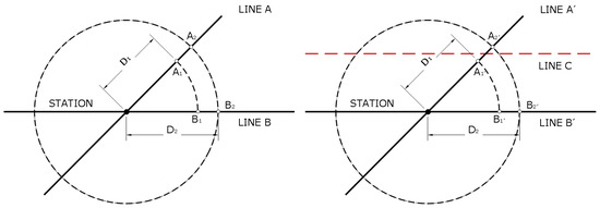 Figure 8. The impact of accessible variables on house price.
wherein
and represent different houses on line A
and represent different houses on line B
and () represent the distance from properties to the closet rail station
represents house price of n and represents the difference in house prices on line N
If and other variables of and are the same, then .
If closeness (line A) > closeness (line B), and other variables are the same, then we can obtain
If and add line C to intersect line A to make line A(B) turn into line and
0 with others are the same, then
5.2. Discussions of Limitation
This study verifies how house price is affected by rail accessibility and road accessibility, as well as the interaction of both through the linear regression interaction model and spatial interaction term model, and reveals the mutual regulating role of accessibility variables on house prices. However, there are some shortcomings. Specifically, it is a complicated process to analyze the impact of interaction on house prices. Furthermore, cities are abundant in specific spatial location functions, and unique, which will change the extent of the influence of the interaction on house prices [43]. Unfortunately, limited by data source, personal abilities, and research time, this study fails to analyze problems comprehensively as follows.
First of all, the sample data selected are too narrow to fully reflect realities in Fuzhou. The findings should be verified further, and this decreases the fitting degree of the equation, affecting the coefficient of the regression equation thereby. In future research, continuous efforts should be made to collect more sample data and improve comprehensiveness of explanatory variables of house prices, so as to come to a more convincing finding with stronger explanatory power.
Then, when the hedonic price model is introduced to analyze house prices, characteristic explanatory variables omit relevant information and have deficiencies, which will reduce the accuracy of hedonic price model in decomposing real prices [44]. As a result, future scholars should consider more components that affect house prices, and split original components elaborately, in order to present a more realistic hedonic price model.
Next, the spatial interactive regression model is promoted because it is related to the spatial autocorrelation of explained variables and spatial disturbance correlation in error terms, without considerations on the spatial autocorrelation of all explanatory variables. In other words, the spatial Durbin model (SDM) is not mentioned or promoted over the general nested space model (GNS) to analyze the applicability of interaction between explanatory variables on the impact of house prices.
Finally, research findings are drawn based on a general traffic development law of cities — construction of subway traffic is slower than ideal construction speed. However, in reality, construction and development speed is diverse for different construction parts of cities, so, this implies that research findings should be analyzed dialectically. At the same time, it is hoped more scholars can study related fields to propose more suggestions and thoughts for model innovation and improvement, and supplement interaction theories of existing house price regression models.
5.3. Conclusions of Implication
In accordance with research purpose and results, this study will explain how to apply these research findings for government, individuals and scholars.
5.3.1. Policy Implications
In terms of third finding, it is recommended that governments should consider balanced urban development, the benefits of subway transportation, and fair transportation when planning subway transportation routes and subway stations. Apart from playing the role of organization, subway lines can stimulate the development of surrounding areas, including economic benefits, infrastructure, and guidance of population flow. If subway lines are arranged along the road network with high proximity, imbalance of this orientation will deteriorate, so that rising of spatial value of subway traffic declines. In summary, Fuzhou should allocate subway transportation lines and subway stations in urban areas with relatively low road network proximity. This will promote the balanced development of cities and provide urban residents with living spaces with better accessibility under low purchase costs. In addition the government can formulate targeted tax policies for areas near the built rail stations. By taking advantage of the population and economic vitality brought by rail stations, the investment in the previous transportation construction is recovered, which can form a virtuous economic cycle and promote urban construction and development.
5.3.2. Personal Implications
According to the fifth finding, when , then , and ; that is, the above formula (a) can be regarded as a transformation of so is obtained. Similarly, is acquired according to . Therefore, the following suggestions are given to buyers: in most cases, when road construction is faster than subway network construction; that is, similar to the above simulation of adding line C, only a single variable (distance between the closet subway station and house) can be considered. Buyers should purchase properties far away from subway stations in light of existing budgets, which is hopeful to improve the potential appreciation of properties. On the other hand, according to the overall level of Fuzhou, people relying more on subway transportation should purchase residential communities within 1800 m of subway stations. Otherwise, people have to pay more for housing expenses because they must rely on roads. Based on the above judgments, home buyers may need to combine their own economic budget and traffic preferences to determine the distance between the purchased residence and the rail station.
In the other hand, under the circumstances of same distance to subway stations but different road network proximity, in what kind of residential communities on road should one buy a house, in order to ensure the highest market value of properties held by buyers in the future? This issue should be discussed under different cases. In Fuzhou, when the subway station is within 1800 m of the residence, the price of properties on roads with smaller increases in road network proximity will be higher than that with significant improvement in road network proximity. The opposite is true beyond 1800 m; in other words, on roads with a smaller increase in road network proximity, the price will be lower than that with significant improvement in road network proximity. In summary, under the same distance to a subway station, residential communities closer to subway stations (within dependent distance) should be built on roads without much road development space, while those in the distance (beyond the dependent distance) are recommended to be constructed on streets with sufficient space for reserve roads construction. According to the above suggestions, home buyers will be able to obtain more residential investment income in the future.
5.3.3. Scholar Implications
The findings of this study partly explain the differences in the findings of previous scholars on similar issues, and also provide ideas for the academic community to study related issues. Previously, many scholars, such as Xin Wei et al. [45] and Zhengyi Zhou et al. [46], respectively studied the regional differences in the impact rail stations on house prices in Chengdu and Shanghai, and gave reasons for the differences. However, the inherent differences of the location variables discussed in their study are more likely to be caused by the different road network accessibility attached to the location variables. This study not only corroborates the authenticity of previous scholars’ research, but also reveals the more essential reasons behind the location variables and improves the theory of the difference in the impact of subway stations on house prices. Moreover, researchers can use similar research ideas to study the differences in the impact of subway stations on house prices in the future, by building interactive regression models for other linear variables.
Since the development of nonlinear models, the use of this method to discuss various problems has been very extensive, both in the field of natural sciences and social sciences. The model can better explain the correlation between multiple variables, optimizing the incompleteness of variable classification discussions, simplifying the complexity, and promoting disciplinary exchanges. Therefore, the discussion of nonlinear models can also be extended to more discussions on price research [47]. In addition, transportation factors are affecting our lives in a more diverse and subtle way, so other scholars are called on to explore the development of transportation systems from the perspective of sustainable optimization in the future [48].
Author Contributions
Conceptualization, K.C. and H.L.; methodology, K.C., H.L. and L.L.; software, K.C. and L.L.; validation, K.C., Y.L. and Z.L.; formal analysis, K.C. and Y.L.; investigation, L.L. and Y.L.; resources, L.L.; data curation, L.L., L.T. and A.W.; writing—original draft preparation, K.C. and Y.L.; writing—review and editing, K.C.; visualization, K.C.; supervision, Y.-J.C.; project administration, L.L.; funding acquisition, L.L. and T.F. All authors have read and agreed to the published version of the manuscript.
Funding
This research was funded by [Distinguished Youth Program of Fujian Agriculture and Forestry University] grant number [XJQ201932] and [Interdisciplinary Integration Guidance Project of College of Landscape Architecture, Fujian Agriculture and Forestry University] grant number [YSYL-xkjc-3].
Institutional Review Board Statement
Not applicable.
Informed Consent Statement
Not applicable.
Conflicts of Interest
The authors declare no conflict of interest.
References
- Yang, L.; Chau, K.W.; Wang, X. Are low-end housing purchasers more willing to pay for access to public services? Evidence from China. Res. Transp. Econ. 2019, 76, 100734. [Google Scholar] [CrossRef]
- Yang, L.; Wang, B.; Zhang, Y.; Ye, Z.; Wang, Y.; Li, P. Willing to pay more for high-quality schools? A hedonic pricing and propensity score matching approach. Int. Rev. Spat. Plan. Sustain. Dev. 2018, 6, 45–62. [Google Scholar]
- Jia, J.; Zhang, X.; Huang, C.; Luan, H. Multiscale analysis of human social sensing of urban appearance and its effects on house price appreciation in Wuhan, China. Sustain. Cities Soc. 2022, 81, 103844. [Google Scholar] [CrossRef]
- Yang, L.; Wang, B.; Zhou, J.; Wang, X. Walking accessibility and property prices. Transp. Res. Part D Transp. Environ. 2018, 62, 551–562. [Google Scholar] [CrossRef]
- Tan, R.; He, Q.; Zhou, K.; Xie, P. The Effect of New Metro Stations on Local Land Use and Housing Prices: The Case of Wuhan, China. J. Transp. Geogr. 2019, 79, 102488. [Google Scholar] [CrossRef]
- Cengiz, E.C.; Çelik, H.M. Investigation of the Impact of Railways on Housing Values; the Case of Istanbul, Turkey. Int. J. Transp. Dev. Integr. 2019, 3, 295–305. [Google Scholar] [CrossRef]
- Law, S. Defining Street-based Local Area and Measuring its Effect on House Price Using a Hedonic Price Approach: The case Study of Metropolitan London. Cities 2017, 60, 166–179. [Google Scholar] [CrossRef]
- Liang, J.; Koo, K.M.; Lee, C.L. Transportation infrastructure improvement and real estate value: Impact of level crossing removal project on housing prices. Transportation 2021, 48, 2969–3011. [Google Scholar] [CrossRef]
- Lin, J.J.; Hwang, C.H. Analysis of Property Prices before and After the Opening of the Taipei Subway System. Ann. Reg. Sci. 2004, 38, 687–704. [Google Scholar] [CrossRef]
- Yang, L.; Chau, K.W.; Chu, X. Accessibility-based premiums and proximity-induced discounts stemming from bus rapid transit in China: Empirical evidence and policy implications. Sustain. Cities Soc. 2019, 48, 101561. [Google Scholar] [CrossRef]
- Medda, F. Land value capture finance for transport accessibility: A review. J. Transp. Geogr. 2012, 25, 154–161. [Google Scholar] [CrossRef]
- Medda, F. Evaluation of Value Capture Mechanisms as a Funding Source for Urban Transport: The Case of London’s Crossrail. Procedia-Soc. Behav. Sci. 2012, 48, 2393–2404. [Google Scholar]
- Lee, C.L.; Locke, M. The effectiveness of passive land value capture mechanisms in funding infrastructure. J. Prop. Investig. Financ. 2021, 39, 283–293. [Google Scholar] [CrossRef]
- Yang, L.; Liang, Y.; Zhu, Q.; Chu, X. Machine learning for inference: Using gradient boosting decision tree to assess non-linear effects of bus rapid transit on house prices. Ann. GIS 2021, 27, 273–284. [Google Scholar] [CrossRef]
- Ridker, R.G.; Henning, J.A. The Determinants of Residential Property Values with Special Reference to Air Pollution. Rev. Econ. Stat. 1967, 49, 246–257. [Google Scholar] [CrossRef]
- Shyr, O.; Andersson, D.E.; Wang, J.; Huang, T.; Liu, O. Where Do Home Buyers Pay Most for Relative Transit Accessibility? Hong Kong, Taipei and Kaohsiung Compared. Urban Stud. 2013, 50, 2553–2568. [Google Scholar] [CrossRef]
- Cui, N.; Gu, H.; Shen, T.; Feng, C. The Impact of Micro-Level Influencing Factors on Home Value: A Housing Price-Rent Comparison. Sustainability 2018, 10, 4343. [Google Scholar] [CrossRef]
- Zou, C.; Tai, J.; Chen, L.; Che, Y. An Environmental Justice Assessment of the Waste Treatment Facilities in Shanghai: Incorporating Counterfactual Decomposition into the Hedonic Price Model. Sustainability 2020, 12, 3325. [Google Scholar] [CrossRef]
- Hitaj, C.; Lynch, L.; McConnell, K.E.; Tra, C.I. The Value of Ozone Air Quality Improvements to Renters: Evidence from Apartment Building Transactions in Los Angeles County. Ecol. Econ. 2018, 146, 721. [Google Scholar] [CrossRef]
- Wang, J.; Lee, C.L. The value of air quality in housing markets: A comparative study of housing sale and rental markets in China. Energy Policy. 2022, 160, 112601. [Google Scholar] [CrossRef]
- Agarwal, S.; Rengarajan, S.; Sing, T.F.; Yang, Y. School allocation rules and housing prices: A quasi-experiment with school relocation events in Singapore. Reg. Sci. Urban Econ. 2016, 58, 56. [Google Scholar] [CrossRef]
- Agarwal, S.; Koo, K.M. Impact of electronic road pricing (ERP) changes on transport modal choice. Reg. Sci. Urban Econ. 2016, 60, 11. [Google Scholar] [CrossRef]
- Xu, T. Heterogeneity in Housing Attribute Prices: A study of the Interaction Behaviour between Property Specifics, Location Coordinates and Buyers’ Characteristics. Int. J. Hous. Mark. Anal. 2008, 1, 166–181. [Google Scholar] [CrossRef]
- Currie, J.; Davis, L.; Greenstone, M.; Walker, R. Environmental Health Risks and Housing Values: Evidence from 1,600 Toxic Plant Openings and Closings. Am. Econ. Rev. 2015, 105, 678–709. [Google Scholar] [CrossRef] [PubMed]
- Im, J.; Hong, S.H. Impact of a New Subway Line on Housing Values in Daegu, Korea: Distance from Existing Lines. Urban Stud. 2018, 55, 3318–3335. [Google Scholar] [CrossRef]
- Mayer, T.; Trevien, C. The impact of urban public transportation evidence from the Paris region. J. Urban Econ. 2017, 102, 1–21. [Google Scholar] [CrossRef]
- Zheng, J.; Liu, H. The Impact of URRT on House Prices in Shenzhen. J. China Railw. Soc. 2005, 27, 11–18. (In Chinese) [Google Scholar]
- Zhang, X.; Jiang, Y. An Empirical Study of the Impact of Metro Station Proximity on Property Value in the Case of Nanjing, China. Asian Dev. Policy Rev. 2014, 2, 61–71. [Google Scholar] [CrossRef]
- Almosaind, M.A.; Dueker, K.J.; Strathman, J.G. Light-rail Transit Stations and Property Values: A Hedonic Price Approach. Transp. Res. Rec. 1993, 1400, 90–94. [Google Scholar]
- Wen, H.; Gui, Z.; Tian, C.; Xiao, Y.; Fang, L. Subway Opening, Traffic Accessibility, and Housing Prices: A Quantile Hedonic Analysis in Hangzhou, China. Sustainability 2018, 10, 2254. [Google Scholar] [CrossRef]
- Armstrong, R.J.; Rodriguez, D.A. An evaluation of the accessibility benefits of commuter rail in eastern Massachusetts using spatial hedonic price functions. Transportation 2006, 33, 21–43. [Google Scholar] [CrossRef]
- Yang, L.; Chen, Y.; Xu, N.; Zhao, R.; Chau, K.W.; Hong, S. Place-varying Impacts of Urban Rail Transit On Property Prices In Shenzhen, China: Insights for value capture. Sustain. Cities Soc. 2020, 58, 102140. [Google Scholar] [CrossRef]
- Matthews, J.W.; Turnbull, G.K. Neighborhood Street Layout and Property Value: The Interaction of Accessibility and Land Use Mix. J. Real Estate Financ. 2007, 35, 111–141. [Google Scholar] [CrossRef]
- Xiao, Y.; Orford, S.; Webster, C.J. Urban Configuration, Accessibility, and Property Prices: A Case Study of Cardiff, Wales. Environ. Plan. B Plan. Des. 2016, 43, 108–129. [Google Scholar] [CrossRef]
- Shen, Y.; Karimi, K. The Economic Value of Streets: Mix-scale Spatio-functional Interaction and Housing Price Patterns. Appl. Geogr. 2017, 79, 187–202. [Google Scholar] [CrossRef]
- Xiao, Y.; Li, Z.; Song, X. Estimating the Value of Street Layout via Local Housing Market: A Empirical Study of Nanjing, China. Urban Dev. Stud. 2015, 22, 6–11. (In Chinese) [Google Scholar]
- Yang, Y.; Li, T.; Feng, X. Analysis on the Pattern of the House Price and Its Driving Forces in the Dwelling Space in the Urban District of Xi’an. Areal Res. Dev. 2015, 34, 68–74. (In Chinese) [Google Scholar]
- Gu, H.; Meng, X.; Shen, T.; Chen, H.; Xiao, F. A Study on the Influrence of Urban Road Network on the Housing Price in Guangzhou Based on sDNA Model. Mod. Urban Res. 2018, 6, 2–8. (In Chinese) [Google Scholar]
- Gu, H.; Lin, Z.; Shen, T.; Mengzhen, H.; Liu, Z. Study on the Highway Network of Urban Agglomeration in the Middle Reaches of the Yangtze River Based on Space Syntax Theory. Areal Res. Dev. 2018, 37, 24–29. (In Chinese) [Google Scholar]
- Liu, X.; Zhu, T. Analysis on the Applicability of Hedonic Price Method in Real Estate Valuation. Foreign Econ. Relat. Trade 2020, 0, 61–63. (In Chinese) [Google Scholar]
- Yang, L.; Zhou, J.; Shyr, O.F.; Huo, D.D. Does Bus Accessibility Affect Property Prices? Cities 2019, 84, 56–65. [Google Scholar] [CrossRef]
- Cervero, R.; Duncan, M. Land value impacts of rail transit services in Los Angeles County. In Report Prepared for National Association of Realtors; Urban Land Institute: Washington, DC, USA, 2002. [Google Scholar]
- Yang, L.; Chau, K.W.; Szeto, W.Y.; Cui, X.; Wang, X. Accessibility to transit, by transit, and property prices: Spatially varying relationships. Transp. Res. Part D Transp. Environ. 2020, 85, 102387. [Google Scholar] [CrossRef]
- Yang, L.; Chu, X.; Gou, Z.; Yang, H.; Lu, Y.; Huang, W. Accessibility and proximity effects of bus rapid transit on housing prices: Heterogeneity across price quantiles and space. J. Transp. Geogr. 2020, 88, 102850. [Google Scholar] [CrossRef]
- Wei, X.; Zhang, W.; Wang, C.; Xu, G. The Impact of Urban Rail Transit on Surrounding Residential Prices--Line 1 of Chengdu Metro as an Example. Modern Appl. Sci. 2012, 6, 58. (In Chinese) [Google Scholar] [CrossRef][Green Version]
- Zhou, Z.; Chen, H.; Zhang, A. The Effect of a Subway on House Prices: Evidence from Shanghai: The Effect of a Subway on House Prices. Real Estate Econ. 2019, 49, 199. (In Chinese) [Google Scholar] [CrossRef]
- Hu, Z.; Legeza, V.P.; Dychka, I.A.; Legeza, D.V. Mathematical Modeling of the Process of Vibration Protection in a System with two-mass Damper Pendulum. Int. J. Intell. Syst. Appl. 2017, 9, 18–25. [Google Scholar] [CrossRef]
- Ahmed, N.; Rabbi, S.; Rahman, T.; Mia, R.; Rahman, M. Traffic Sign Detection and Recognition Model Using Support Vector Machine and Histogram of Oriented Gradient. Int. J. Inf. Technol. Comput. Sci. 2021, 13, 61–73. [Google Scholar] [CrossRef]
Publisher’s Note: MDPI stays neutral with regard to jurisdictional claims in published maps and institutional affiliations. |
© 2022 by the authors. Licensee MDPI, Basel, Switzerland. This article is an open access article distributed under the terms and conditions of the Creative Commons Attribution (CC BY) license (https://creativecommons.org/licenses/by/4.0/).