Pricing Policy in an Inventory Model with Green Level Dependent Demand for a Deteriorating Item

Abstract

The goal of this research is to investigate an inventory model for degrading commodities with linear selling prices and nonlinear green level-dependent demand for an item. The pre-payment option with a one-time flat reduction on the product’s selling price is considered here. The governing differential equations are used to mathematically define the model and solve numerically to optimize the model’s average profit. After that, the model is tested using a numerical example, and sensitivity analyses are run to see how changing inventory factors affects the best strategy. The concavity of the objective function is shown graphically with the help of MATLAB software. Finally, some applications of this approach and future scopes are discussed.

1. Introduction

The best inventory policy has a tremendous influence on every aspect of company management. Different inventory characteristics, such as demand rate, degradation rate, preservation technology, ordering cost, holding cost, backlog parameter, greenness, and so on, play a significant part in determining the best strategy.

The usage of various chemicals and preservatives in the manufacture of everyday items is continually rising as manufacturing technologies of various credentials are enhanced. The majority of these chemicals and preservatives are dangerous to human health and seem to be the root of several ailments. Customers’ attention has been attracted to green goods and their advantages as a result of this reality. Green goods are described as varieties of sustainable products that are meant to have the least possible effect on the environment or human health over their entire life cycle, including after usage. Green goods are primarily characterized by an indicator known as “green level”, which is based on three key factors: (i) environmentally friendly manufacturing; (ii) items that are more health-friendly; and (iii) the usage of these products generates little or no pollution. In the present market context, there is a rising positive influence of green credentials on-demand, i.e., the number of green product customers is fast expanding. Over the past several decades, there has been a tremendous increase in studies concerning the impact of green products on the market economy. A couple of these studies are detailed in this article. Taleizadeh et al. [1] investigated the combined optimum policy of product selling price and replenishment frequency in a green product manufacturing inventory model. Hammami et al. [2] investigated the impact of carbon emissions in a multi-echelon green product manufacturing inventory model. Khatua and Maity [3] also looked at the impact of product greenness on demand and the link between profit and pollution in an imperfect production inventory system. Golari et al. [4] investigated a multistage optimization issue for a production model using intermittent renewable green energy sources. Saxena et al. [5] developed a fuzzy logic-based eco-friendly green inventory model. Yavari and Geraeli [6] proposed a heuristic solution for handling the green-supply chain’s resilient optimization challenge. Sana [7] then looked at the pricing rivalry between green and non-green items made by a socially responsible company. Sarker et al. [8] then looked at the environmental and economic sustainability of a green product manufacturing company. Paul et al. [9] developed a green buying model that took into account the impact of carbon taxes. Green investment was examined by Jauhari and Wangsa [10] in a manufacturer-retailer supply chain model.

An item’s demand rate might be either constant or changing. Variable demand is influenced by a variety of factors, such as the selling price, supply level, product greenness, time, and so on. The variable demand rate may increase or decrease as a consequence of various variables. The demand rate and other inventory costs were assumed to be constant in Harris’s basic EOQ model [11]. Several academics examined numerous forms of requests in their suggested inventory models after that time. Here, are some of the most fascinating pieces among them. Ritchie [12] used a linear growing demand model to investigate an EOQ model. Pal and Chaudhuri [13] looked into deterministic inventory with stock-linked demand. Wee [14] investigated a model with price-dependent demand and its replenishment strategy. A two-warehouse inventory model with a time-dependent demand rate was developed by Lee and Ying [15]. Miranda and Garrido [16] investigated a random demand inventory issue. Maihami and Kamalabadi [17] looked at a joint pricing inventory model with a time and price-dependent demand rate. Abdul Rahim et al. [18] used stochastic demand to address the multi-period inventory routing issue. Nagaraju et al. [19] looked at a two-echelon inventory model with a demand that was price dependent. Sarkar et al. [20] investigated a preservation technology-based inventory model for degrading products with stock-dependent demand rates. Pervin et al. [21], Shaikh et al. [22], Mondal et al. [23], Rahman et al. [24], and others have recently published papers in this field.

Deterioration/decay is a natural process in which things lose their freshness and qualitative attributes, such as vegetables, food, and beverages. Though the rate of decay cannot be predicted precisely, many scholars assumed it to be either constant, time-dependent, imprecise, random, or a combination of these. The researchers proposed preservation technology principles in the domain of inventory management since irresponsible degradation might have a negative impact on the ideal strategy. In addition, there are other works in the current literature that deal with this idea. Several relevant works are addressed among them. Raafat [25] conducted a survey of the literature on inventory models with continual degradation. Chang and Dye [26] investigated an inventory model for decaying items with a reasonable amount of time to deteriorate. Bhunia and Shaikh [27] investigated a deterministic inventory model for continuously decaying objects. In their suggested paradigm for decaying goods, Hsieh and Dye [28] presented the notion of preservation technology. For degrading objects under preservation technology, Rossetti et al. [29] investigated the impact of the demand of (r, q) inventory model. Tayal et al. [30] presented the ideal strategy of a two-echelon inventory model. Dye and Yang [31] investigated the impact of preservation investment on the best policy of a perishable commodities inventory model. In the field of inventory management, Khan et al. [32], Shaikh et al. [33], Das et al. [34], Rahman et al. [35,36], and others have recently submitted their work.

Advance payment is a sensible business approach for a businessman or a corporation to limit the risk of their business. Customers must pay for order amounts in advance under this policy. This approach is most often used when demand for a product is strong, and the market is experiencing a crisis. This strategy might also be used with a discount facility in typical market demand. There are many works on advanced payment and discount facilities in the extant literature, including in their supply chain model. Chen [37] included an advanced payment mechanism to investigate the best policy. Cachon [38] looked at the impact of advanced payment policies and discount facilities on a supply chain model’s optimum policy. In their inventory model with a random lead time, Maiti et al. [39] included an advanced payment policy. Taleizadeh et al. [40] looked at a discount inventory system. Zhang et al. [41] developed a model for estimating economic order quantities with advance payment. Teng et al. [42] investigated the lot-size rules for degrading products with advance payments in an inventory issue. The advanced payment and discount services were recently studied by Tavakoli and Taleizadeh [43], Soto et al. [44], Wu et al. [45], Shaikh et al. [46], Khan et al. [47,48,49], Rahman et al. [50], Khan et al. [51], Duary et al. [52], Manna et al. [53], Khan et al. [54], and others.

In inventory management, the cost of holding is a critical factor. To keep the product in good condition up to the end of the business period, the retailer must invest some money. As a result, the optimum strategy is heavily influenced by this cost. Other cost considerations, such as ordering cost, purchase cost, shortfall cost, lost sale cost, and so on, have a significant influence on the best lot size. These variables are assumed to be constant in most cases. Several academics looked at several sorts of holding costs to determine the best policy for the inventory model. Chang [55], Tripathy and Mishra [56], Mishra et al. [57], Dutta and Kumar [58], Alfares and Ghaithan [59], Rastogi et al. [60], Cárdenas-Barrón et al. [61], and Das et al. [62] are only a few of them.

After a deep survey of the literature, in this work, an EOQ model for decaying commodities is developed, with selling price and nonlinear green level dependent. The influence of greenness is taken into consideration in this formulation. Additionally, taken into account is the ability to pay in advance as well as a one-time reduction in the product’s price. The suggested model’s associated average profit is then solved mathematically with the help of one numerical example and proved the optimality theoretically. The following is how the paper is structured:

The issue definition, assumptions, and nomenclature are presented in Section 2. The mathematical formulation of the model, as well as the solution technique are described in Section 3. The numerical examples and sensitivity assessments are accomplished in Section 4. Finally, in Section 5, the study is summarized and ended.

2. Description of Problem, Notation, and Assumptions

2.1. Description

Consider a scenario in which the seller offers an early payment discount. In this case, the customer pays for the items in installments before receiving them. Then, at the time of prepayment, he or she receives a set percentage, say $\mu \%$ a discount, off the entire purchase price. It goes without saying that in order to benefit from the early payment discount, customers must have adequate cash on hand. Furthermore, some clients operate their businesses with limited cash reserves and must take a bank loan at a certain interest rate. Buyers must prepare for payment before receiving products under the advanced payment method. The purchasers’ capital is made up of this payable money. This money is not always readily accessible to the purchasers. In this circumstance, purchasers will need to borrow money via bank loans or other financial organizations along with terms and conditions in order to keep the firm functioning smoothly. This is in addition to their capital cost. When a customer prepays, he or she receives a discount on the total purchase cost of the items (a specified percentage) immediately in cash. To maintain his or her consumers, the vendor accepts the buyer’s proposal and gives a discount on the whole amount of the purchase price paid in advance.

2.2. Notation

To study the model in a proper way, the notation and assumptions used are given in Appendix A.

2.3. Assumptions

1.

Greenness is the most important issue in the current business scenario. Here, we assumed a deteriorated green product whose demand is dependent on price and nonlinear green level and it is mathematically represented as $D(p,g)=a-bp+c{g}^{\lambda }$ where $a,b,c,\lambda >0$ and the value of green level ($g$) is measured within the interval (0,1). For analysis of this nonlinear model, we may refer the works of Grabinski and Klinkova [63] and Klinkova and Grabinski [64];

2.

The rate of decaying $\delta (0<\delta <<1)$ is fixed (Khan et al. [32] and Shaikh et al. [33]);

3.

Replenishment rate is infinite and lead time is $M$ (Shaikh et al. [46], Khan et al. [32], Rahman et al. [50], Khan et al. [47,48], Duary et al. [52], Manna et al. [53]);

4.

During the time under consideration, there is no replacement or repair for degraded items;

5.

The total inventory planning horizon is infinite;

6.

When a buyer pays his or her purchase price before receiving the items at time $M$, he or she receives a percentage $\mu$ reduction off the total purchase price at the moment of prepayment.

3. Model Formulation and Solution Procedure

In this situation, the consumer buys the items in advance by paying the whole purchase price before receiving the lot. At first, a customer buys items, Q units, by paying the entire purchase price before receiving the products from a seller that offers an early payment discount. The inventory level is depleted due to the joint effect of demand $D(p,g)$, as well as the deterioration, and at time $t=T$ stock becomes zero. Thus, the proposed model satisfied the given differential equation

$$\frac{dI(t)}{dt}+\delta I(t)=-D(p,g), 0\le t\le t_1$$

(1)

with the boundary conditions $I(0)=Q$ and $I(T)=0$.

Solving Equation (1) with the help of boundary condition $I(T)=0$, we have

$$I(t)=\frac{D(p,g)}{\delta }\left\{e^{\delta (T-t)}-1\right\}$$

(2)

Using the condition $I(0)=Q$, the highest stock is as:

$$Q=\frac{D(p,g)}{\delta }\left\{e^{\delta T}-1\right\}$$

(3)

Thus, the total ordering quantity is $(Q)$ units. Therefore, the total purchasing cost for the buyer is calculated with $c(Q)$. Since the buyer prepays the full purchasing cost at the time $M$ before receiving a lot, he/she obtains a certain percentage $\mu \%$ discount of the total purchasing cost for prepaying amount. As a consequence, the lower purchase price and the accompanying loan cost are calculated as $(1-\mu )c(Q)$ and $I_{e}M(1-\mu )c(Q)$, respectively.

The components of the total cost are:

a.

Ordering cost: $K_o$

b.

Purchasing cost (PC): $\left(1-\mu \right)c\left(Q\right)$

c.

Holding cost (HC): $c_h{\displaystyle \underset{0}{\overset{T}{\int }}I\left(t\right)dt}=c_h\frac{D(p,g)}{{\delta }^2}\left\{e^{\delta T}-\delta T-1\right\}$

d.

Cost of loan (COL): $I_{e}M(1-\mu )c(Q)$

e.

Greening cost (GC)=$\eta gT$

f.

Sales revenue (SR)=$p{\displaystyle \underset{0}{\overset{T}{\int }}D(p,g)dt}=p{\displaystyle \underset{0}{\overset{T}{\int }}\left(a-bp+c{g}^{\lambda }\right)}dt$$=p\left(a-bp+c{g}^{\lambda }\right)T$

The total profit is given by:

$$TP=SR-K_0-PC-HC-COL-GC$$

(4)

Hence, the total profit per unit time is:

$$\pi (p,g,T)=\frac{TP}{T}.$$

(5)

i.e.,

$$\pi (p,g,T)=\frac{1}{T}\left[p\left(a-bp+c{g}^{\lambda }\right)T-\left\{\begin{array}{l}{K}_0+\left(1-\mu \right)c_p\frac{\left(a-bp+c{g}^{\lambda }\right)}{\delta }\left\{e^{\delta T}-1\right\}+\frac{c_h\left(a-bp+c{g}^{\lambda }\right)}{{\delta }^2}\left\{e^{\delta T}-\delta T-1\right\}\\ +I_{e}M(1-\mu )c_p\frac{\left(a-bp+c{g}^{\lambda }\right)}{\delta }\left\{e^{\delta T}-1\right\}+\eta gT\end{array}\right\}\right]$$

(6)

The corresponding optimization problem can be written as

$$\begin{array}{l}Maximize \pi (p,g,T)\\ subject to p>0, T>0\end{array}$$

(7)

Now, it is observed that problem (7) is highly nonlinear in nature along with four decision variables. To show the problem optimality analytically is quite a complicated task. For this reason, the proposed model is solved with the help of MATHEMATICA software.

4. Theoretical Derivations

The concavity of the total profit function is discussed of Equation (6) some findings from Cambini and Martein were utilized to analyse the model’s concavity (2009). The function of the form is based on Cambini and Martein [65]’s Theorems 3.2.9 and 3.2.10.

$$\prod (u)=\frac{f(u)}{g(u)},u\in {ℝ}^n$$

If f(x) is a negative, differentiable, and (strictly) concave function but g(x) is a positive, differentiable, and concave function, it is (strictly) pseudo-concave. We can prove that the total profit function (6) is a strictly pseudo-concave function of T using this approach, and we can find the unique optimum solution T* that maximizes the total profit function (6).

Here, we need to investigate the concavity of the objective function $\pi (p,g,T)$ with respect to $p,g \mathrm{and} T$

where

$$f(p,g,T)=\left[p\left(a-bp+c{g}^{\lambda }\right)T-\left\{\begin{array}{l}{K}_0+\left(1-\mu \right)c_p\frac{\left(a-bp+c{g}^{\lambda }\right)}{\delta }\left\{e^{\delta T}-1\right\}+\frac{c_h\left(a-bp+c{g}^{\lambda }\right)}{{\delta }^2}\left\{e^{\delta T}-\delta T-1\right\}\\ +I_{e}M(1-\mu )c_p\frac{\left(a-bp+c{g}^{\lambda }\right)}{\delta }\left\{e^{\delta T}-1\right\}+\eta gT\end{array}\right\}\right]$$

(8)

and

$$g(p,g,T)=T$$

(9)

Lemma 1. 

Total profit function π(p,g,T) is strictly pseudo-concave if

$$2bT\left[\begin{array}{l}\left(1-\mu \right)c_p\frac{c\lambda \left(\lambda -1\right)g^{\lambda -1}}{\delta }\left\{e^{\delta T}-1\right\}+\frac{c_{h}c\lambda \left(\lambda -1\right)g^{\lambda -1}}{{\delta }^2}\left\{e^{\delta T}-\delta T-1\right\}\\ +I_{e}M(1-\mu )c_p\frac{c\lambda \left(\lambda -1\right)g^{\lambda -1}}{\delta }\left\{e^{\delta T}-1\right\}\end{array}\right]>2bT\left(pc\lambda \left(\lambda -1\right)g^{\lambda -1}T\right)+{\lambda }^2{c}^2{g}^{2\lambda -2}{T}^2$$

Proof. 

Differentiate Equation (8) with respect to p and g, we obtain

$$\frac{\partial f(.)}{\partial p}=\left(a-bp+c{g}^{\lambda }\right)T-bpT+\left(1-\mu \right)c_p\frac{b}{\delta }\left\{e^{\delta T}-1\right\}+\frac{c_{h}b}{{\delta }^2}\left\{e^{\delta T}-\delta T-1\right\}+I_{e}M(1-\mu )c_p\frac{b}{\delta }\left\{e^{\delta T}-1\right\},$$

$$\frac{\partial f(p,g,T)}{\partial g}=pc\lambda g^{\lambda -1}T-\left(1-\mu \right)c_p\frac{c\lambda g^{\lambda -1}}{\delta }\left\{e^{\delta T}-1\right\}-\frac{c_{h}c\lambda g^{\lambda -1}}{{\delta }^2}\left\{e^{\delta T}-\delta T-1\right\}-I_{e}M(1-\mu )c_p\frac{c\lambda g^{\lambda -1}}{\delta }\left\{e^{\delta T}-1\right\}-\eta T,$$

$$\frac{{\partial }^{2}f(.)}{\partial p\partial g}=\lambda c{g}^{\lambda -1}T$$

and

$$\frac{{\partial }^{2}f(p,g,T)}{\partial g^2}=\left[\begin{array}{l}pc\lambda \left(\lambda -1\right)g^{\lambda -1}T-\left(1-\mu \right)c_p\frac{c\lambda \left(\lambda -1\right)g^{\lambda -1}}{\delta }\left\{e^{\delta T}-1\right\}-\frac{c_{h}c\lambda \left(\lambda -1\right)g^{\lambda -1}}{{\delta }^2}\left\{e^{\delta T}-\delta T-1\right\}\\ -I_{e}M(1-\mu )c_p\frac{c\lambda \left(\lambda -1\right)g^{\lambda -1}}{\delta }\left\{e^{\delta T}-1\right\}\end{array}\right]$$

Second principal minor

$$\begin{array}{l}\left|H_{22}\right|=\frac{{\partial }^{2}f(.)}{\partial p^2}\frac{{\partial }^{2}f(.)}{\partial g^2}-{\left(\frac{{\partial }^{2}f(.)}{\partial p\partial g}\right)}^2>0 \mathrm{if}\\ \left(-2bT\right)\left[\begin{array}{l}pc\lambda \left(\lambda -1\right)g^{\lambda -1}T-\left(1-\mu \right)c_p\frac{c\lambda \left(\lambda -1\right)g^{\lambda -1}}{\delta }\left\{e^{\delta T}-1\right\}-\frac{c_{h}c\lambda \left(\lambda -1\right)g^{\lambda -1}}{{\delta }^2}\left\{e^{\delta T}-\delta T-1\right\}\\ -I_{e}M(1-\mu )c_p\frac{c\lambda \left(\lambda -1\right)g^{\lambda -1}}{\delta }\left\{e^{\delta T}-1\right\}\end{array}\right]-{\left(\lambda c{g}^{\lambda -1}T\right)}^2>0\\ 2bT\left[\begin{array}{l}\left(1-\mu \right)c_p\frac{c\lambda \left(\lambda -1\right)g^{\lambda -1}}{\delta }\left\{e^{\delta T}-1\right\}+\frac{c_{h}c\lambda \left(\lambda -1\right)g^{\lambda -1}}{{\delta }^2}\left\{e^{\delta T}-\delta T-1\right\}\\ +I_{e}M(1-\mu )c_p\frac{c\lambda \left(\lambda -1\right)g^{\lambda -1}}{\delta }\left\{e^{\delta T}-1\right\}\end{array}\right]>2bT\left(pc\lambda \left(\lambda -1\right)g^{\lambda -1}T\right)+{\lambda }^2{c}^2{g}^{2\lambda -2}{T}^2\end{array}$$

□

Lemma 2. 

Total profit function π(p,g,T) is strictly pseudo-concave if

$$\left\{\begin{array}{l}\frac{{\partial }^{2}f(.)}{\partial p^2}\frac{{\partial }^{2}f(.)}{\partial g^2}\frac{{\partial }^{2}f(.)}{\partial T^2}+\frac{{\partial }^{2}f(.)}{\partial p\partial g}\frac{{\partial }^{2}f(.)}{\partial g\partial T}\frac{{\partial }^{2}f(.)}{\partial p\partial T}\\ +\frac{{\partial }^{2}f(.)}{\partial p\partial T}\frac{{\partial }^{2}f(.)}{\partial p\partial g}\frac{{\partial }^{2}f(.)}{\partial g\partial T}\end{array}\right\}<\left\{\begin{array}{l}\frac{{\partial }^{2}f(.)}{\partial p^2}\frac{{\partial }^{2}f(.)}{\partial g\partial T}\frac{{\partial }^{2}f(.)}{\partial g\partial T}+\frac{{\partial }^{2}f(.)}{\partial p\partial g}\frac{{\partial }^{2}f(.)}{\partial p\partial g}\frac{{\partial }^{2}f(.)}{\partial T^2}\\ +\frac{{\partial }^{2}f(.)}{\partial p\partial T}\frac{{\partial }^{2}f(.)}{\partial g^2}\frac{{\partial }^{2}f(.)}{\partial p\partial T}\end{array}\right\}$$

Proof. 

Let us consider the hessian matrix of the function f(p,g,T) is

$$H=\left[\begin{array}{ccc}\frac{{\partial }^{2}f(.)}{\partial p^2}& \frac{{\partial }^{2}f(.)}{\partial p\partial g}& \frac{{\partial }^{2}f(.)}{\partial p\partial T}\\ \frac{{\partial }^{2}f(.)}{\partial p\partial g}& \frac{{\partial }^{2}f(.)}{\partial g^2}& \frac{{\partial }^{2}f(.)}{\partial g\partial T}\\ \frac{{\partial }^{2}f(.)}{\partial p\partial T}& \frac{{\partial }^{2}f(.)}{\partial g\partial T}& \frac{{\partial }^{2}f(.)}{\partial T^2}\end{array}\right]$$

and the corresponding determinant value is

$$\left|H\right|=\left|\begin{array}{ccc}\frac{{\partial }^{2}f(.)}{\partial p^2}& \frac{{\partial }^{2}f(.)}{\partial p\partial g}& \frac{{\partial }^{2}f(.)}{\partial p\partial T}\\ \frac{{\partial }^{2}f(.)}{\partial p\partial g}& \frac{{\partial }^{2}f(.)}{\partial g^2}& \frac{{\partial }^{2}f(.)}{\partial g\partial T}\\ \frac{{\partial }^{2}f(.)}{\partial p\partial T}& \frac{{\partial }^{2}f(.)}{\partial g\partial T}& \frac{{\partial }^{2}f(.)}{\partial T^2}\end{array}\right|<0$$

Now, if we apply the rule of the determinant then

$$\begin{array}{l}\frac{{\partial }^{2}f(.)}{\partial p^2}\left|\begin{array}{cc}\frac{{\partial }^{2}f(.)}{\partial g^2}& \frac{{\partial }^{2}f(.)}{\partial g\partial T}\\ \frac{{\partial }^{2}f(.)}{\partial g\partial T}& \frac{{\partial }^{2}f(.)}{\partial T^2}\end{array}\right|-\frac{{\partial }^{2}f(.)}{\partial p\partial g}\left|\begin{array}{cc}\frac{{\partial }^{2}f(.)}{\partial p\partial g}& \frac{{\partial }^{2}f(.)}{\partial g\partial T}\\ \frac{{\partial }^{2}f(.)}{\partial p\partial T}& \frac{{\partial }^{2}f(.)}{\partial T^2}\end{array}\right|+\frac{{\partial }^{2}f(.)}{\partial p\partial T}\left|\begin{array}{cc}\frac{{\partial }^{2}f(.)}{\partial p\partial g}& \frac{{\partial }^{2}f(.)}{\partial g^2}\\ \frac{{\partial }^{2}f(.)}{\partial p\partial T}& \frac{{\partial }^{2}f(.)}{\partial g\partial T}\end{array}\right|<0\end{array}$$

which follows that

$$\left\{\begin{array}{l}\frac{{\partial }^{2}f(.)}{\partial p^2}\frac{{\partial }^{2}f(.)}{\partial g^2}\frac{{\partial }^{2}f(.)}{\partial T^2}+\frac{{\partial }^{2}f(.)}{\partial p\partial g}\frac{{\partial }^{2}f(.)}{\partial g\partial T}\frac{{\partial }^{2}f(.)}{\partial p\partial T}\\ +\frac{{\partial }^{2}f(.)}{\partial p\partial T}\frac{{\partial }^{2}f(.)}{\partial p\partial g}\frac{{\partial }^{2}f(.)}{\partial g\partial T}\end{array}\right\}<\left\{\begin{array}{l}\frac{{\partial }^{2}f(.)}{\partial p^2}\frac{{\partial }^{2}f(.)}{\partial g\partial T}\frac{{\partial }^{2}f(.)}{\partial g\partial T}+\frac{{\partial }^{2}f(.)}{\partial p\partial g}\frac{{\partial }^{2}f(.)}{\partial p\partial g}\frac{{\partial }^{2}f(.)}{\partial T^2}\\ +\frac{{\partial }^{2}f(.)}{\partial p\partial T}\frac{{\partial }^{2}f(.)}{\partial g^2}\frac{{\partial }^{2}f(.)}{\partial p\partial T}\end{array}\right\}$$

□

Theorem 1.

Total profit function π(p,g,T) is strictly pseudo-concave function with respect to p, g, and T, hence π(p,g,T) archives the global maximum at the point p*, g*, T*.

Proof. 

Using Equations (8) and (9), we have

$$f(p,g,T)=\left[p\left(a-bp+c{g}^{\lambda }\right)T-\left\{\begin{array}{l}{K}_0+\left(1-\mu \right)c_p\frac{\left(a-bp+c{g}^{\lambda }\right)}{\delta }\left\{e^{\delta T}-1\right\}+\frac{c_h\left(a-bp+c{g}^{\lambda }\right)}{{\delta }^2}\left\{e^{\delta T}-\delta T-1\right\}\\ +I_{e}M(1-\mu )c_p\frac{\left(a-bp+c{g}^{\lambda }\right)}{\delta }\left\{e^{\delta T}-1\right\}+\eta gT\end{array}\right\}\right]$$

and

$$g(p,g,T)=T$$

According to Cambini and Martein [65]’s Theorems 3.2.9 and 3.2.10, we need to show that f(p,g,T) is a negative, differentiable and (strictly) joint concave function with respect to p, g and T.

Using Equation (8), we have

$$\frac{\partial f(.)}{\partial p}=\left(a-bp+c{g}^{\lambda }\right)T-bpT+\left(1-\mu \right)c_p\frac{b}{\delta }\left\{e^{\delta T}-1\right\}+\frac{c_{h}b}{{\delta }^2}\left\{e^{\delta T}-\delta T-1\right\}+I_{e}M(1-\mu )c_p\frac{b}{\delta }\left\{e^{\delta T}-1\right\},$$

$$\frac{{\partial }^{2}f(.)}{\partial p^2}=-bT-bT=-2bT,$$

$$\frac{{\partial }^{2}f(.)}{\partial p\partial g}=\lambda c{g}^{\lambda -1}T,$$

$$\frac{{\partial }^{2}f(.)}{\partial p\partial T}=\left(a-bp+c{g}^{\lambda }\right)-bp+\left(1-\mu \right)c_{p}b{e}^{\delta T}+\frac{c_{h}b}{\delta }\left\{e^{\delta T}-1\right\}+I_{e}M(1-\mu )c_{p}b{e}^{\delta T},$$

$$\frac{\partial f(p,g,T)}{\partial g}=pc\lambda g^{\lambda -1}T-\left(1-\mu \right)c_p\frac{c\lambda g^{\lambda -1}}{\delta }\left\{e^{\delta T}-1\right\}-\frac{c_{h}c\lambda g^{\lambda -1}}{{\delta }^2}\left\{e^{\delta T}-\delta T-1\right\}-I_{e}M(1-\mu )c_p\frac{c\lambda g^{\lambda -1}}{\delta }\left\{e^{\delta T}-1\right\}-\eta T,$$

$$\frac{\partial f(p,g,T)}{\partial g\partial T}=pc\lambda g^{\lambda -1}-\left(1-\mu \right)c_{p}c\lambda g^{\lambda -1}{e}^{\delta T}-\frac{c_{h}c\lambda g^{\lambda -1}}{{\delta }^2}\left\{e^{\delta T}-1\right\}-I_{e}M(1-\mu )c_{p}c\lambda g^{\lambda -1}{e}^{\delta T}-\eta$$

$$\frac{{\partial }^{2}f(p,g,T)}{\partial g^2}=\left[\begin{array}{l}pc\lambda \left(\lambda -1\right)g^{\lambda -1}T-\left(1-\mu \right)c_p\frac{c\lambda \left(\lambda -1\right)g^{\lambda -1}}{\delta }\left\{e^{\delta T}-1\right\}-\frac{c_{h}c\lambda \left(\lambda -1\right)g^{\lambda -1}}{{\delta }^2}\left\{e^{\delta T}-\delta T-1\right\}\\ -I_{e}M(1-\mu )c_p\frac{c\lambda \left(\lambda -1\right)g^{\lambda -1}}{\delta }\left\{e^{\delta T}-1\right\}\end{array}\right],$$

$$\frac{\partial f(p,g,T)}{\partial T}=p\left(a-bp+c{g}^{\lambda }\right)-\left(1-\mu \right)c_p\left(a-bp+c{g}^{\lambda }\right)e^{\delta T}-\frac{c_h\left(a-bp+c{g}^{\lambda }\right)}{\delta }\left\{e^{\delta T}-1\right\}-I_{e}M(1-\mu )c_p{c}_p\left(a-bp+c{g}^{\lambda }\right)e^{\delta T}-\eta g$$

$$\frac{{\partial }^{2}f(p,g,T)}{\partial T^2}=-\left(1-\mu \right)c_p\delta \left(a-bp+c{g}^{\lambda }\right)e^{\delta T}-c_h\left(a-bp+c{g}^{\lambda }\right)e^{\delta T}-I_{e}M(1-\mu )c_p\delta \left(a-bp+c{g}^{\lambda }\right)e^{\delta T}$$

Therefore, the hessian matrix of the function f(p,g,T) is given by

$$H=\left[\begin{array}{ccc}\frac{{\partial }^{2}f(.)}{\partial p^2}& \frac{{\partial }^{2}f(.)}{\partial p\partial g}& \frac{{\partial }^{2}f(.)}{\partial p\partial T}\\ \frac{{\partial }^{2}f(.)}{\partial p\partial g}& \frac{{\partial }^{2}f(.)}{\partial g^2}& \frac{{\partial }^{2}f(.)}{\partial g\partial T}\\ \frac{{\partial }^{2}f(.)}{\partial p\partial T}& \frac{{\partial }^{2}f(.)}{\partial g\partial T}& \frac{{\partial }^{2}f(.)}{\partial T^2}\end{array}\right]$$

First principal minor $\left|H_{11}\right|=\frac{{\partial }^{2}f(.)}{\partial p^2}=-bT-bT=-2bT<0$

Second principal minor

$$\left|H_{22}\right|=\frac{{\partial }^{2}f(.)}{\partial p^2}\frac{{\partial }^{2}f(.)}{\partial g^2}-{\left(\frac{{\partial }^{2}f(.)}{\partial p\partial g}\right)}^2>0(\mathrm{using} \mathbf{Lemma} \mathbf{1})$$

Similarly, we are able to show that $\left|H\right|<0$ and, hence, the Hessian matrix of the function $f(p,g,T)$ is negative definite with the help of Lemma 2. Hence, the function $f(p,g,T)$ is a negative, differentiable, and (strictly) concave function with respect to $p,g \mathrm{and} T.$ Additionally, $g(p,g,T)=T>0$ is affine. Therefore, the objective function is pseudo-concave and it attains the global maximum at the point $p^{*},g^{*} \mathrm{and} T^{*}$. □

According to the necessary condition, we have

$$\frac{\partial \pi (p,g,T)}{\partial p}=\frac{1}{T}\left[\left(a-bp+c{g}^{\lambda }\right)T-bpT+\left(1-\mu \right)c\frac{b}{\delta }\left\{e^{\delta T}-1\right\}+\frac{c_{h}b}{{\delta }^2}\left\{e^{\delta T}-\delta T-1\right\}+I_{e}M(1-\mu )c\frac{b}{\delta }\left\{e^{\delta T}-1\right\}\right]=0$$

(10)

$$\frac{\partial \pi (p,g,T)}{\partial g}=\frac{1}{T}\left[pc\lambda g^{\lambda -1}T-\frac{\left(1-\mu \right)c_{p}c\lambda g^{\lambda -1}}{\delta }\left\{e^{\delta T}-1\right\}-\frac{c_{h}c\lambda g^{\lambda -1}}{{\delta }^2}\left\{e^{\delta T}-\delta T-1\right\}-I_{e}M(1-\mu )c_p\frac{c\lambda g^{\lambda -1}}{\delta }\left\{e^{\delta T}-1\right\}-\eta T\right]=0$$

(11)

and

$$\frac{\partial \pi (p,g,T)}{\partial T}=-\frac{TP}{T^2}+\frac{1}{T}\left[\begin{array}{l}p\left(a-bp+c{g}^{\lambda }\right)-\left(1-\mu \right)c_p\left(a-bp+c{g}^{\lambda }\right)e^{\delta T}-\frac{c_h\left(a-bp+c{g}^{\lambda }\right)}{\delta }\left\{e^{\delta T}-1\right\}\\ -I_{e}M(1-\mu )c_p\left(a-bp+c{g}^{\lambda }\right)e^{\delta T}-\eta g\end{array}\right]=0$$

(12)

Proposed Algorithm

In this section, a solution algorithm (see Algorithm 1) is proposed, and one numerical example is considered to justify the reality of the proposed model.

Algorithm 1:

$\mathrm{Step} 1: \mathrm{initialize} \mathrm{all} \mathrm{input} \mathrm{parameters} \mathrm{and} \mathrm{set} \epsilon <0.00001$ $\mathrm{Step} 2: \mathrm{set} p=5 , g=1$ solve Equation (12) and store the value of T $\mathrm{Step} 3: \mathrm{using} \mathrm{the} \mathrm{value} \mathrm{of} T \mathrm{and} p=5$ solve Equation (11) and store the value of g Step 4: using the updated value of T and g solve Equation (10) and store the value of p $\mathrm{Step} 5: \mathrm{repeat} \mathrm{Step} 2 \mathrm{to} \mathrm{Step} 4 \mathrm{until} \mathrm{the} \mathrm{termination} \mathrm{criteria} \mathrm{satisfied}, \mathrm{i}.\mathrm{e}., p_{n+1}-p_n<\epsilon$$, g_{n+1}-g_n<\epsilon$$\mathrm{and} T_{n+1}-T_n<\epsilon$ $\mathrm{Step} 6: \mathrm{store} \mathrm{the} \mathrm{optimal} \mathrm{value} \mathrm{of} p^{*},g^{*} \& T^{*}$ and obtained the optimal vale of the objective function. Step 7: Stop

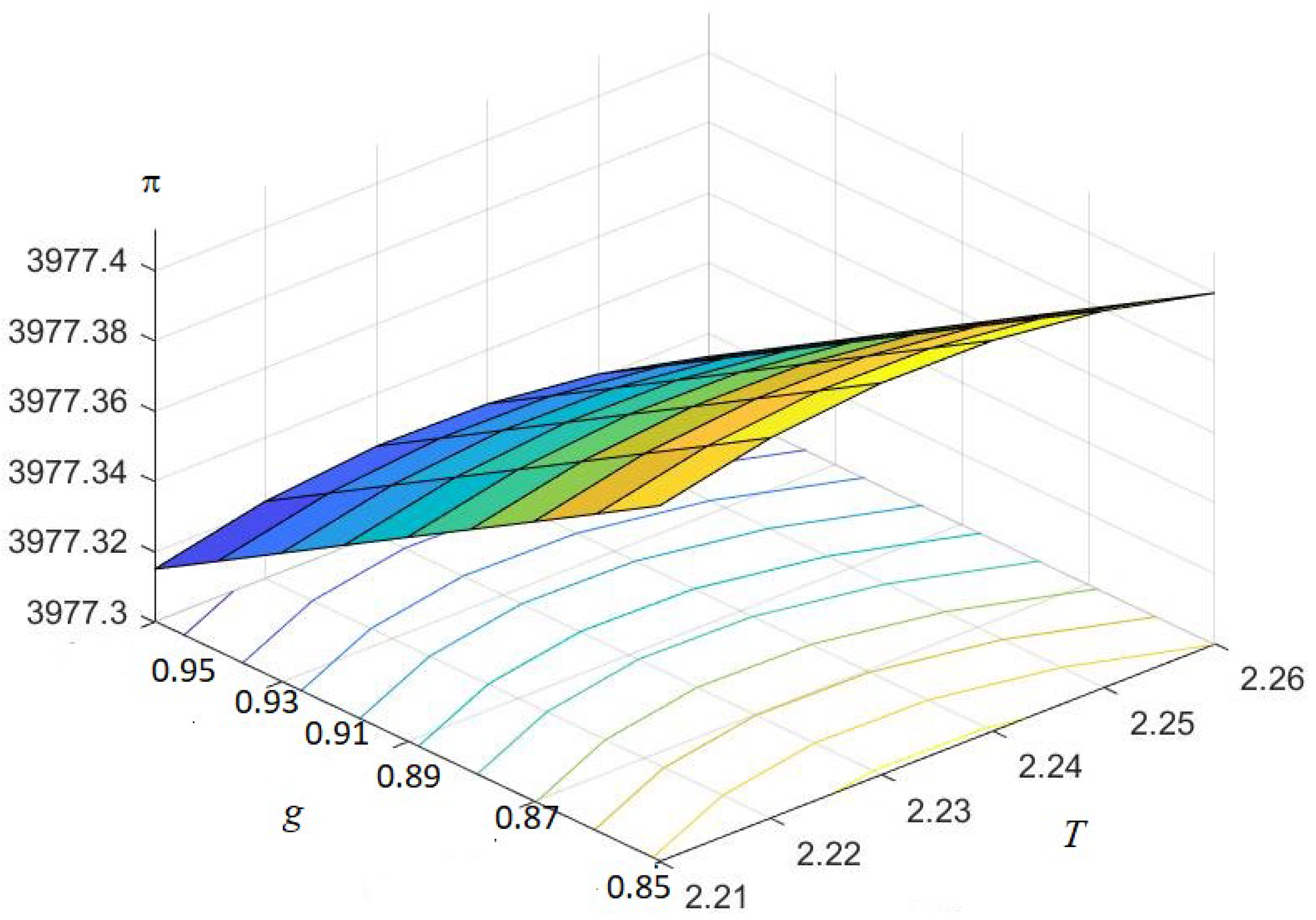
5. Numerical Illustration

In order to validate the proposed model one numerical example is considered. The values of the system parameters are given below and the solutions are presented in

Table 1. Optimal results of Example.

Variables/Unknown Parameters	Optimal Values
$p$	$142.2302
$T$	2.2296
g	0.9167
$\pi$	$3977.4117
$Q$	145.8497

:

Example 1.

The values of the different inventory parameters associated with the proposed model are given below.

$$\begin{array}{l}a=150, b=0.7, c=3,\lambda =0.08,\delta =0.2, M=0.8/year, \mu =0.2, \eta =1.8 K_o=\$350/order\\ , c_p=\$50/unit, c_h=\$1.5/unit/year, I_e=\$0.05/year, g=1\end{array}$$

In addition, the concavity of the objective function is shown graphically by taking two decision variables at a time and one decision variable keeps the optimal value. All the figures are drawn with the help of MATLAB software, and are shown in Figure 1, Figure 2 and Figure 3.

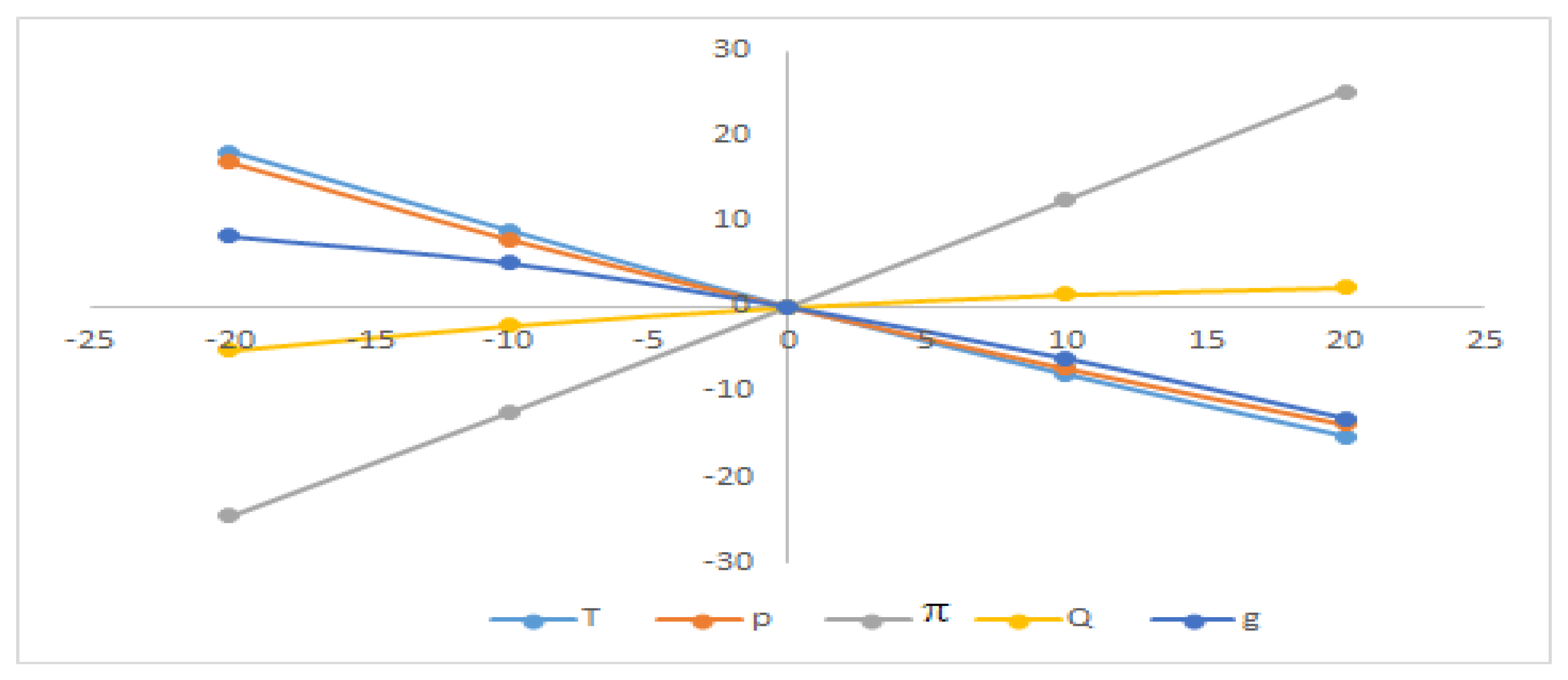
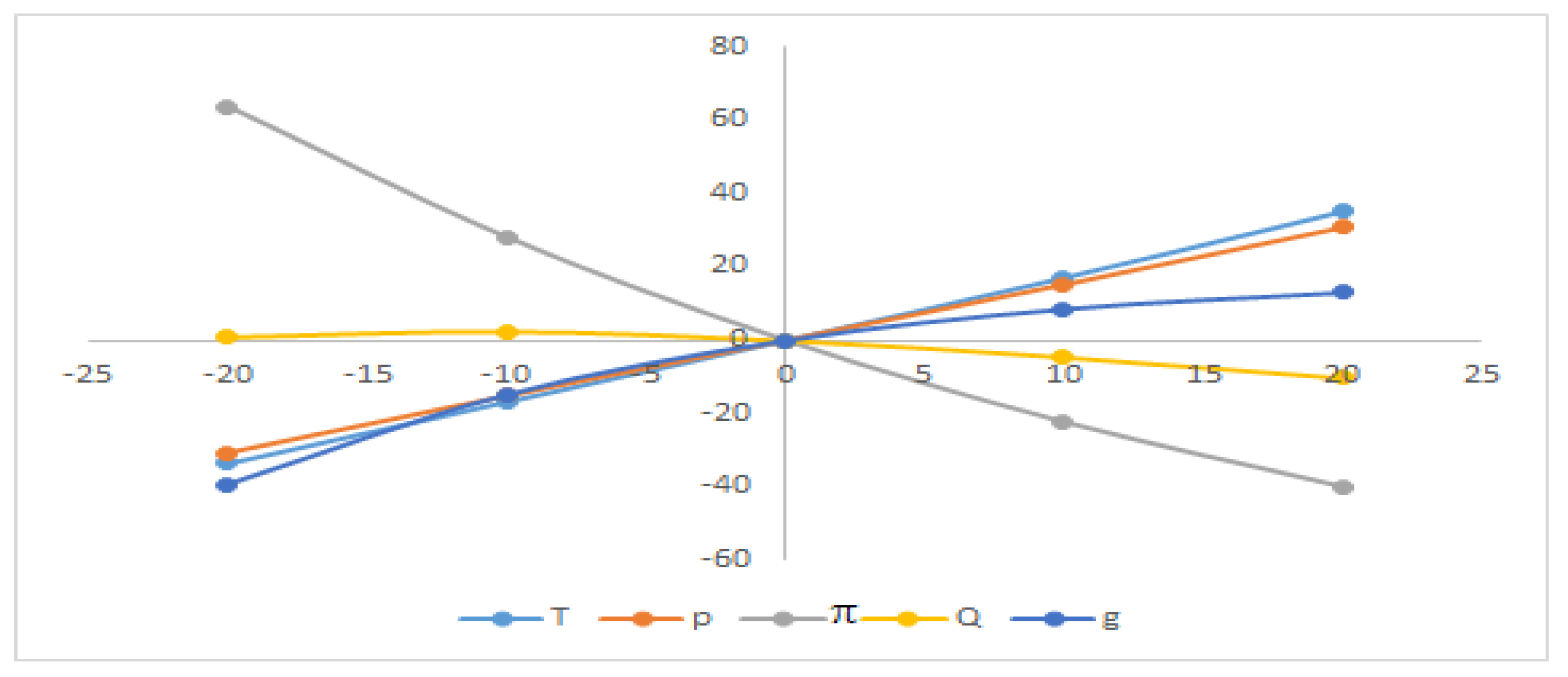
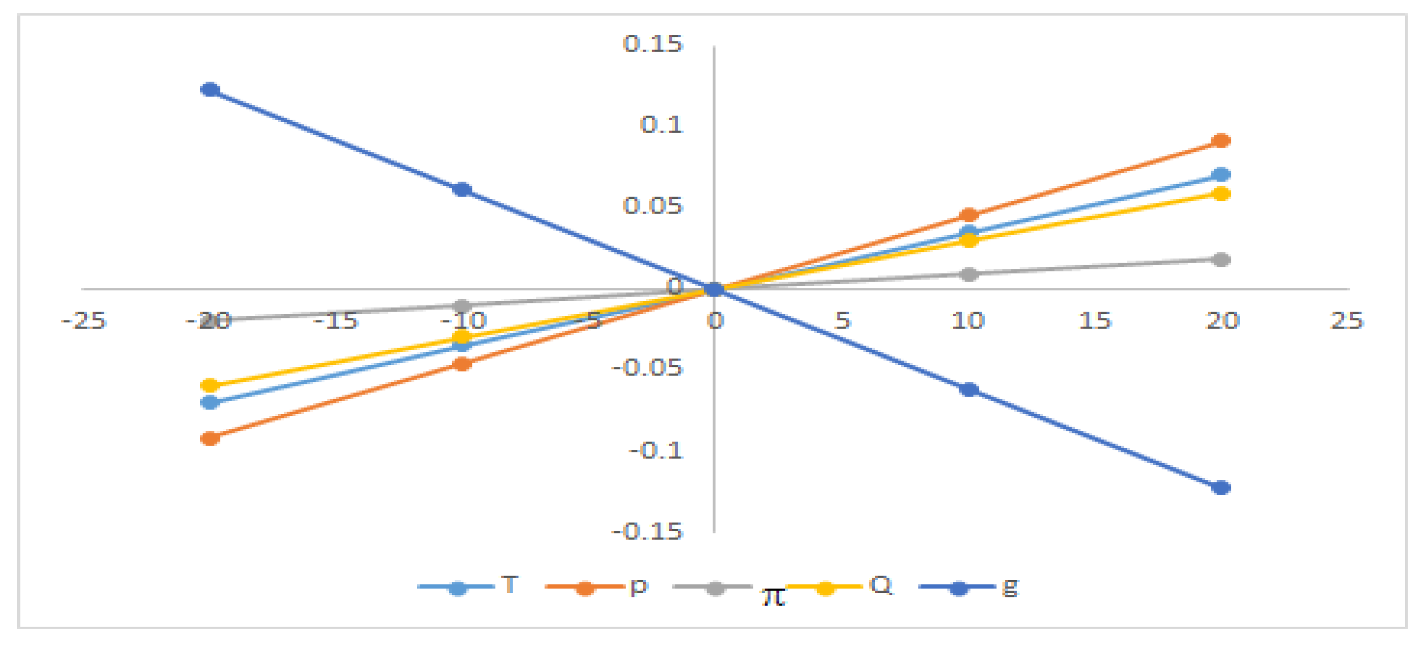
6. Sensitivity Analyses

To show the impact of the various inventory parameters on total cycle length (T), initial stock level ‘$Q$’, maximum green level ‘$g$’, and the average profit ‘$\pi$’, the sensitivity analyses are performed with respect to the numerical Example 1 by changing the values of the parameters from −20% to +20%. The optimal results of these analyses are presented graphically in Figure 4, Figure 5, Figure 6, Figure 7, Figure 8, Figure 9 and Figure 10.

From Figure 4, Figure 5, Figure 6, Figure 7, Figure 8, Figure 9 and Figure 10, the average profit ($\pi$) is highly sensitive to the positive or negative changes of the selling price (p), the location parameter of demand ‘$a$’, and the scaling parameter ‘$b$’ but ‘$\pi$’ has the reverse effect with respect to ‘b’. The average profit ($\pi$) is less sensitive to the positive or negative changes of ordering cost ‘$K_o$’, ‘$\mu$’, and ‘$c_h$’ whereas the average profit ($\pi$) is insensitive to the positive or negative changes of ‘$\delta$’ and ‘$c$’.

From Figure 4, Figure 5, Figure 6, Figure 7, Figure 8, Figure 9 and Figure 10, it is clear that the cycle length ($T$) is highly sensitive to the positive or negative changes of demand parameter ‘$b$’. The cycle length ($T$) is mostly equally sensitive to the positive or negative changes of ordering cost ‘$K_o$’ and the location parameter of demand ‘$a$’, respectively. The cycle length ($T$) is also less sensitive to the positive or negative changes of the selling price ‘p’, constant deterioration rate ‘$\delta$’, and holding cost ‘$c_h$’ but ‘$\delta$’ and ‘$c_h$’ have the reverse effect.

The initial stock level ($Q$) is mostly equally sensitive to the positive or negative changes of ordering cost ‘$K_o$’. The initial stock level ($Q$) is less sensitive to the positive or negative changes of ‘$\theta$’, ‘$h$’ and ‘$a$’, respectively, but ‘$\theta$’ and ‘$h$’ are inversely affected. The initial stock level ($Q$) is insensitive to the positive or negative changes of ‘$\alpha$’, ‘$b$’ and ‘$\mu$’, respectively.

7. Summary

In this work, an EOQ model, for deteriorating items, is formulated by considering the demand rate depending on the linear selling price and nonlinear green level of goods. Consideration of advanced payment with a flat discount facility and greenness-dependent demand makes the model more realistic. Additionally, the green technology investment cost increases the applicability of the proposed model. The concavity of the objective function is shown graphically with the help of MATLAB software. From the sensitivity analyses, it can be concluded that the average profit is significantly effective with respect to the demand scaling parameter, location parameter, and selling price in both positive and negative senses. Thus, a decision-maker/manager should take more care of these parameters during decision-making. The concept of this model can be used in the business sector involving food, vegetables, medicine, etc.

For future work, this model may be extended in imprecise environments (fuzzy, interval, Type-2 interval (Rahman et al. [35]) by taking the uncertainty in the inventory parameters.

References

- Taleizadeh, A.A.; Noori-daryan, M.; Cárdenas-Barrón, L.E. Joint optimization of price, replenishment frequency, replenishment cycle and production rate in vendor managed inventory system with deteriorating items. Int. J. Prod. Econ. 2015, 159, 285–295. [Google Scholar] [CrossRef]
- Hammami, R.; Nouira, I.; Frein, Y. Carbon emissions in a multi-echelon production-inventory model with lead time constraints. Int. J. Prod. Econ. 2015, 164, 292–307. [Google Scholar] [CrossRef]
- Khatua, D.; Maity, K. Research on relationship between economical profit and environmental pollution of imperfect production inventory control problem. J. Niger. Math. Soc. 2016, 35, 560–579. [Google Scholar]
- Golari, M.; Fan, N.; Jin, T. Multistage stochastic optimization for production-inventory planning with intermittent renewable energy. Prod. Oper. Manag. 2017, 26, 409–425. [Google Scholar] [CrossRef]
- Saxena, S.; Gupta, R.K.; Singh, V.; Singh, P.; Mishra, N.K. Environmental Sustainability with eco-friendly green inventory model under Fuzzy logics considering carbon emission. J. Emerg. Technol. Innov. Res. 2018, 5, 1297–1301. [Google Scholar]
- Yavari, M.; Geraeli, M. Heuristic method for robust optimization model for green closed-loop supply chain network design of perishable goods. J. Clean. Prod. 2019, 226, 282–305. [Google Scholar] [CrossRef]
- Sana, S.S. Price competition between green and non green products under corporate social responsible firm. J. Retail. Consum. Serv. 2020, 55, 102118. [Google Scholar] [CrossRef]
- Sarkar, B.; Ullah, M.; Sarkar, M. Environmental and economic sustainability through innovative green products by remanufacturing. J. Clean. Prod. 2021, 2021, 129813. [Google Scholar] [CrossRef]
- Paul, A.; Pervin, M.; Roy, S.K.; Maculan, N.; Weber, G.W. A green inventory model with the effect of carbon taxation. Ann. Oper. Res. 2022, 309, 233–248. [Google Scholar] [CrossRef]
- Jauhari, W.A.; Wangsa, I.D. A Manufacturer-Retailer Inventory Model with Remanufacturing, Stochastic Demand, and Green Investments. Process Integr. Optim. Sustain. 2022, 1–21. [Google Scholar] [CrossRef]
- Harris, F.W. How many parts to make at once. Oper. Res. 1913, 38, 947–950, reprinted in Fact. Mag. Manag. 1913, 10, 135–136. [Google Scholar] [CrossRef]
- Ritchie, E. The EOQ for linear increasing demand: A simple optimal solution. J. Oper. Res. Soc. 1984, 35, 949–952. [Google Scholar] [CrossRef]
- Pal, S.; Goswami, A.; Chaudhuri, K.S. A deterministic inventory model for deteriorating items with stock-dependent demand rate. Int. J. Prod. Econ. 1993, 32, 291–299. [Google Scholar] [CrossRef]
- Wee, H.M. A replenishment policy for items with a price-dependent demand and a varying rate of deterioration. Prod. Plan. Control. 1997, 8, 494–499. [Google Scholar] [CrossRef]
- Lee, C.C.; Ying, C. Optimal inventory policy for deteriorating items with two-warehouse and time-dependent demands. Prod. Plan. Control. 2000, 11, 689–696. [Google Scholar] [CrossRef]
- Miranda, P.A.; Garrido, R.A. Incorporating inventory control decisions into a strategic distribution network design model with stochastic demand. Transp. Res. Part E Logist. Transp. Rev. 2004, 40, 183–207. [Google Scholar] [CrossRef]
- Maihami, R.; Kamalabadi, I.N. Joint pricing and inventory control for non-instantaneous deteriorating items with partial backlogging and time and price dependent demand. Int. J. Prod. Econ. 2012, 136, 116–122. [Google Scholar] [CrossRef]
- Abdul Rahim, M.K.I.; Zhong, Y.; Aghezzaf, E.H.; Aouam, T. Modelling and solving the multiperiod inventory-routing problem with stochastic stationary demand rates. Int. J. Prod. Res. 2014, 52, 4351–4363. [Google Scholar] [CrossRef]
- Nagaraju, D.; Rao, A.R.; Narayanan, S. Optimal lot sizing and inventory decisions in a centralised and decentralised two echelon inventory system with price dependent demand. Int. J. Logist. Syst. Manag. 2015, 20, 1–23. [Google Scholar] [CrossRef]
- Sarkar, B.; Mandal, B.; Sarkar, S. Preservation of deteriorating seasonal products with stock-dependent consumption rate and shortages. J. Ind. Manag. Optim. 2017, 13, 187. [Google Scholar] [CrossRef] [Green Version]
- Pervin, M.; Roy, S.K.; Weber, G.W. Analysis of inventory control model with shortage under time-dependent demand and time-varying holding cost including stochastic deterioration. Ann. Oper. Res. 2018, 260, 437–460. [Google Scholar] [CrossRef]
- Shaikh, A.A.; Bhunia, A.K.; Cárdenas-Barrón, L.E.; Sahoo, L.; Tiwari, S. A fuzzy inventory model for a deteriorating item with variable demand, permissible delay in payments and partial backlogging with shortage follows inventory (SFI) policy. Int. J. Fuzzy Syst. 2018, 20, 1606–1623. [Google Scholar] [CrossRef]
- Mondal, R.; Shaikh, A.A.; Bhunia, A.K. Crisp and interval inventory models for ameliorating item with Weibull distributed amelioration and deterioration via different variants of quantum behaved particle swarm optimization-based techniques. Math. Comput. Model. Dyn. Syst. 2019, 25, 602–626. [Google Scholar] [CrossRef]
- Rahman, M.S.; Duary, A.; Shaikh, A.A.; Bhunia, A.K. An application of parametric approach for interval differential equation in inventory model for deteriorating items with selling-price-dependent demand. Neural Comput. Appl. 2020, 32, 14069–14085. [Google Scholar] [CrossRef]
- Raafat, F. Survey of literature on continuously deteriorating inventory models. J. Oper. Res. Soc. 1991, 42, 27–37. [Google Scholar] [CrossRef]
- Chang, H.J.; Dye, C.Y. An inventory model for deteriorating items with partial backlogging and permissible delay in payments. Int. J. Syst. Sci. 2001, 32, 345–352. [Google Scholar] [CrossRef]
- Bhunia, A.; Shaikh, A. A deterministic model for deteriorating items with displayed inventory level dependent demand rate incorporating marketing decisions with transportation cost. Int. J. Ind. Eng. Comput. 2011, 2, 547–562. [Google Scholar] [CrossRef]
- Hsieh, T.P.; Dye, C.Y. A production–inventory model incorporating the effect of preservation technology investment when demand is fluctuating with time. J. Comput. Appl. Math. 2013, 239, 25–36. [Google Scholar] [CrossRef]
- Rossetti, M.D.; Shbool, M.; Varghese, V.; Pohl, E. Investigating the Effect of Demand Aggregation on the Performance of An (R, Q) Inventory Control Policy. In Proceedings of the 2013 Winter Simulations Conference (WSC), Washington, DC, USA, 8–11 December 2013; pp. 3318–3329. [Google Scholar]
- Tayal, S.; Singh, S.R.; Sharma, R.; Chauhan, A. Two echelon supply chain model for deteriorating items with effective investment in preservation technology. Int. J. Math. Oper. Res. 2014, 6, 84–105. [Google Scholar] [CrossRef]
- Dye, C.Y.; Yang, C.T. Optimal dynamic pricing and preservation technology investment for deteriorating products with reference price effects. Omega 2016, 62, 52–67. [Google Scholar] [CrossRef]
- Khan, M.A.A.; Shaikh, A.A.; Panda, G.C.; Konstantaras, I. Two-warehouse inventory model for deteriorating items with partial backlogging and advance payment scheme. RAIRO-Oper. Res. 2019, 53, 1691–1708. [Google Scholar] [CrossRef]
- Shaikh, A.A.; Das, S.C.; Bhunia, A.K.; Panda, G.C.; Al-Amin Khan, M. A two-warehouse EOQ model with interval-valued inventory cost and advance payment for deteriorating item under particle swarm optimization. Soft Comput. 2019, 23, 13531–13546. [Google Scholar] [CrossRef]
- Das, S.C.; Zidan, A.M.; Manna, A.K.; Shaikh, A.A.; Bhunia, A.K. An application of preservation technology in inventory control system with price dependent demand and partial backlogging. Alex. Eng. J. 2020, 59, 1359–1369. [Google Scholar]
- Rahman, M.S.; Shaikh, A.A.; Bhunia, A.K. On Type-2 interval with interval mathematics and order relations: Its applications in inventory control. Int. J. Syst. Sci. Oper. Logist. 2020, 8, 283–295. [Google Scholar] [CrossRef]
- Rahman, M.S.; Manna, A.K.; Shaikh, A.A.; Bhunia, A.K. An application of interval differential equation on a production inventory model with interval-valued demand via center-radius optimization technique and particle swarm optimization. Int. J. Intell. Syst. 2020, 35, 1280–1326. [Google Scholar] [CrossRef]
- Chen, F. Market segmentation, advanced demand information, and supply chain performance. Manuf. Serv. Oper. Manag. 2001, 3, 53–67. [Google Scholar] [CrossRef]
- Cachon, G.P. The allocation of inventory risk in a supply chain: Push, pull, and advance-purchase discount contracts. Manag. Sci. 2004, 50, 222–238. [Google Scholar] [CrossRef] [Green Version]
- Maiti, A.K.; Maiti, M.K.; Maiti, M. Inventory model with stochastic lead-time and price dependent demand incorporating advance payment. Appl. Math. Model. 2009, 33, 2433–2443. [Google Scholar] [CrossRef]
- Taleizadeh, A.A.; Niaki, S.T.A.; Aryanezhad, M.B.; Tafti, A.F. A genetic algorithm to optimize multiproduct multiconstraint inventory control systems with stochastic replenishment intervals and discount. Int. J. Adv. Manuf. Technol. 2010, 51, 311–323. [Google Scholar] [CrossRef]
- Zhang, Q.; Tsao, Y.C.; Chen, T.H. Economic order quantity under advance payment. Appl. Math. Model. 2014, 38, 5910–5921. [Google Scholar] [CrossRef]
- Teng, J.T.; Cárdenas-Barrón, L.E.; Chang, H.J.; Wu, J.; Hu, Y. Inventory lot-size policies for deteriorating items with expiration dates and advance payments. Appl. Math. Model. 2016, 40, 8605–8616. [Google Scholar] [CrossRef]
- Tavakoli, S.; Taleizadeh, A.A. An EOQ model for decaying item with full advanced payment and conditional discount. Ann. Oper. Res. 2017, 259, 415–436. [Google Scholar] [CrossRef]
- Soto, A.V.; Chowdhury, N.T.; Allahyari, M.Z.; Azab, A.; Baki, M.F. Mathematical modeling and hybridized evolutionary LP local search method for lot-sizing with supplier selection, inventory shortage, and quantity discounts. Comput. Ind. Eng. 2017, 109, 96–112. [Google Scholar] [CrossRef]
- Wu, J.; Teng, J.T.; Chan, Y.L. Inventory policies for perishable products with expiration dates and advance-cash-credit payment schemes. Int. J. Syst. Sci. Oper. Logist. 2018, 5, 310–326. [Google Scholar] [CrossRef]
- Shaikh, A.A.; Khan, M.A.A.; Panda, G.C.; Konstantaras, I. Price discount facility in an EOQ model for deteriorating items with stock-dependent demand and partial backlogging. Int. Trans. Oper. Res. 2019, 26, 1365–1395. [Google Scholar] [CrossRef]
- Khan, M.A.A.; Shaikh, A.A.; Panda, G.C.; Konstantaras, I.; Taleizadeh, A.A. Inventory system with expiration date: Pricing and replenishment decisions. Comput. Ind. Eng. 2019, 132, 232–247. [Google Scholar] [CrossRef]
- Khan, M.A.A.; Shaikh, A.A.; Panda, G.C.; Konstantaras, I.; Cárdenas-Barrón, L.E. The effect of advance payment with discount facility on supply decisions of deteriorating products whose demand is both price and stock dependent. Int. Trans. Oper. Res. 2020, 27, 1343–1367. [Google Scholar] [CrossRef]
- Khan, M.; Shaikh, A.A.; Panda, G.C.; Bhunia, A.K.; Konstantaras, I. Non-instantaneous deterioration effect in ordering decisions for a two-warehouse inventory system under advance payment and backlogging. Ann. Oper. Res. 2020, 289, 243–275. [Google Scholar] [CrossRef]
- Rahman, M.S.; Khan, M.A.A.; Halim, M.A.; Nofal, T.A.; Shaikh, A.A.; Mahmoud, E.E. Hybrid price and stock dependent inventory model for perishable goods with advance payment related discount facilities under preservation technology. Alex. Eng. J. 2021, 60, 3455–3465. [Google Scholar] [CrossRef]
- Khan, M.A.A.; Shaikh, A.A.; Cárdenas-Barrón, L.E. An inventory model under linked-to-order hybrid partial advance payment, partial credit policy, all-units discount and partial backlogging with capacity constraint. Omega 2021, 103, 102418. [Google Scholar] [CrossRef]
- Duary, A.; Das, S.; Arif, M.G.; Abualnaja, K.M.; Khan, M.A.A.; Zakarya, M.; Shaikh, A.A. Advance and delay in payments with the price-discount inventory model for deteriorating items under capacity constraint and partially backlogged shortages. Alex. Eng. J. 2022, 61, 1735–1745. [Google Scholar] [CrossRef]
- Manna, A.K.; Khan, M.A.A.; Rahman, M.S.; Shaikh, A.A.; Bhunia, A.K. Interval valued demand and prepayment-based inventory model for perishable items via parametric approach of interval and meta-heuristic algorithms. Knowl. Based Syst. 2022, 242, 108343. [Google Scholar] [CrossRef]
- Khan, M.A.A.; Halim, M.A.; AlArjani, A.; Shaikh, A.A.; Uddin, M.S. Inventory management with hybrid cash-advance payment for time-dependent demand, time-varying holding cost and non-instantaneous deterioration under backordering and non-terminating situations. Alex. Eng. J. 2022, 61, 8469–8486. [Google Scholar] [CrossRef]
- Chang, C.T. Inventory models with stock-dependent demand and nonlinear holding costs for deteriorating items. Asia-Pac. J. Oper. Res. 2004, 21, 435–446. [Google Scholar] [CrossRef]
- Tripathy, C.K.; Mishra, U. An inventory model for Weibull deteriorating items with price dependent demand and time-varying holding cost. Appl. Math. Sci. 2010, 4, 2171–2179. [Google Scholar]
- Mishra, V.K.; Singh, L.S.; Kumar, R. An inventory model for deteriorating items with time-dependent demand and time-varying holding cost under partial backlogging. J. Ind. Eng. Int. 2013, 9, 4. [Google Scholar] [CrossRef] [Green Version]
- Dutta, D.; Kumar, P. A partial backlogging inventory model for deteriorating items with time-varying demand and holding cost: An interval number approach. Croat. Oper. Res. Rev. 2015, 7, 281–296. [Google Scholar] [CrossRef]
- Alfares, H.K.; Ghaithan, A.M. Inventory and pricing model with price-dependent demand, time-varying holding cost, and quantity discounts. Comput. Ind. Eng. 2016, 94, 170–177. [Google Scholar] [CrossRef]
- Rastogi, M.; Singh, S.; Kushwah, P.; Tayal, S. An EOQ model with variable holding cost and partial backlogging under credit limit policy and cash discount. Uncertain Supply Chain. Manag. 2017, 5, 27–42. [Google Scholar] [CrossRef]
- Cárdenas-Barrón, L.E.; Shaikh, A.A.; Tiwari, S.; Treviño-Garza, G. An EOQ inventory model with nonlinear stock dependent holding cost, nonlinear stock dependent demand and trade credit. Comput. Ind. Eng. 2020, 139, 105557. [Google Scholar] [CrossRef]
- Das, S.; Khan, M.A.A.; Mahmoud, E.E.; Abdel-Aty, A.H.; Abualnaja, K.M.; Shaikh, A.A. A production inventory model with partial trade credit policy and reliability. Alex. Eng. J. 2021, 60, 1325–1338. [Google Scholar] [CrossRef]
- Grabinski, M.; Klinkova, G. Wrong use of averages implies wrong results from many heuristic models. Appl. Math. 2019, 10, 605. [Google Scholar] [CrossRef] [Green Version]
- Klinkova, G.; Grabinski, M. A Statistical Analysis of Games with No Certain Nash Equilibrium Make Many Results Doubtful. Appl. Math. 2022, 13, 120–130. [Google Scholar] [CrossRef]
- Cambini, A.; Martein, L. Generalized Convexity and Optimization: Theory and Applications, 1st ed.; Springer: Berlin/Heidelberg, Germany, 2009. [Google Scholar]