Robust Optimization for a Bi-Objective Green Closed-Loop Supply Chain with Heterogeneous Transportation System and Presorting Consideration

Abstract

In this study, we propose a robust bi-objective optimization model of the green closed-loop supply chain network considering presorting, a heterogeneous transportation system, and carbon emissions. The proposed model is an uncertain bi-objective mixed-integer linear optimization model that maximizes profit and minimizes carbon emissions by considering uncertain costs, selling price, and carbon emissions. The robust optimization approach is implemented using the combined interval and polyhedral, “Interval+ Polyhedral,” uncertainty set to develop the robust counterpart of the proposed model. Robust Pareto optimal solutions are obtained using a lexicographic weighted Tchebycheff optimization approach of the bi-objective model. Intensive computational experiments are conducted and a robust Pareto optimal front is obtained with a probability guarantee that the constraints containing uncertain parameters are not violated (constraint satisfaction).

1. Introduction

In April of 2018, the concentration of carbon dioxide, CO${}_2$, in the atmosphere reached 410 parts per million (ppm), which was the highest level in the previous 800,000 years; compared to the previous highest level in 1780 which was just 280 ppm [1,2]. Many crises have resulted from carbon emissions, including rising sea levels and accelerating species extinction [2,3].

The transportation sector was the second-largest source of CO${}_2$ emissions in 2018, around 25% of the total carbon emissions, according to a report by the International Energy Agency [4]. As a result, limiting transportation’s excessive CO${}_2$ emission growth has become a critical component of global CO${}_2$ emission reduction [5].

Many governments pay attention to conducting measures and refining legislation to motivate organizations and a broad sector of customers to adopt green and sustainable practices in their production and service activities [6,7]. Approximately 197 countries at the UN climate summit in November 2021 agreed on new measures for carbon emission reduction, including standards for reporting national emissions and the ground rules for trading credits [8].

A green closed-loop supply chain (GCLSC) involves the integration of environmental aspects into all activities of the traditional closed-loop supply chain (CLSC) network [9,10]. Recently, customers’ behavior has remarkably changed. They are concerned about the environmental aspects of the products and their price and quality [11,12].

Numerous companies are pursuing greenness and sustainability by employing inspection, recycling, and refurbishing activities to recover the used products collected from end customers to increase their return rates [13]. For instance, Xerox, Canon, Kodak, Dell, and Acer have been pushing green operations. For example, by the year 2012, Xerox had effectively cut their emissions by 42% and their energy consumption by 31% [14].

Transportation fleets that move goods between supply chain hubs are a significant contributor to rising environmental consequences. According to Golicic et al. [15], fleet management has a favorable influence on energy efficiency and reduces fleet-related environmental consequences.

Using a heterogeneous fleet comprised of vehicles of varied sizes, the amount of fuel required to serve a given request portfolio can be drastically reduced [16]. Moreover, it provides a better balance of economic and environmental sustainability simultaneously [17,18].

Government policymakers should incentivize businesses to collect used products from customer zones for reverse logistics activities that in turn consolidate greenness and sustainability [19]. Considering efficient presorting centers at the customer zones substantially separates the low-quality returned products at the early stage from the refurbishment stream, thereby causing a reduction in the induced cost and carbon emissions [20].

Most real-life optimization problems are multi-objective and, usually, are uncertain due to the inherent errors of parameter values [21]. These errors result from inappropriate measurement or estimation due to a lack of knowledge of parameter values [22], a highly dynamic environment, and the physical impossibility to implement a computing solution in real-life problems [23]. Ignoring these uncertainties in optimization problems leads to infeasible and sub-optimal solutions [24].

Stochastic optimization (SO) and robust optimization (RO) are well-known approaches for solving uncertain optimization problems. In the SO approach, the probability of uncertain parameters must be defined accurately, but precisely defining this probability is difficult [23,25]. In addition, this approach devastates the convexity property and alleviates the complexity of the original problem in the chance constraints. However, in the RO approach, the uncertainty of the parameter is predefined in an uncertainty set characterized by its shape and size, and this approach overcomes some drawbacks of the SO approach [26].

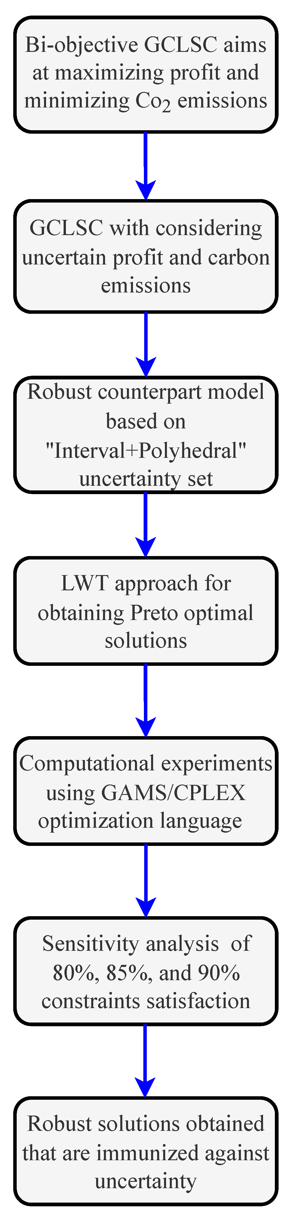
As far as we are aware, few studies [27,28,29] have focused on the RO-based multi-objective optimization of CLSC networks. In these investigations, the implemented uncertainty set is the box uncertainty set with a homogeneous transportation system and no presorting centers in client zones. Motivated by the above facts, we developed a bi-objective robust optimization model for the GCLSC by considering presorting and heterogeneous transportation systems. The logical interpretation of the proposed study’s framework is depicted in Figure 1. The main contributions of this study are as follows:

• Presenting a bi-objective mixed-integer linear programming (MILP) model for the GCLSC while considering presorting and a heterogeneous transportation system as well as uncertain cost, selling price, and carbon emissions uncertainties.
• Presenting a robust counterpart model formulation of the bi-objective MILP model of the GCLSC network under uncertainties using the well-known RO approach based on the "Interval + Polyhedral" uncertainty set.
• Performing intensive computational experiments using a lexicographic weighted Tchebycheff (LWT) approach to obtain the Pareto optimal solutions of the robust bi-objective model, in which the probability bounds on constraint satisfaction are not violated.

The remainder of this paper is organized as follows. Section 2 presents the relevant literature pertaining to the uncertain GCLSC model from the previous studies. Section 3 discusses the problem description and mathematical modeling of the bi-objective GCLSC model. Section 4 presents the robust counterpart formulation of the bi-objective GCLSC model based on the combined "Interval+Polyhedral" uncertainty set. Section 5 presents the solution approach, LWT approach, and the conducted computational experiments. Finally, the conclusion and possible recommendations for future work are presented in Section 6.

2. Relevant Literature

Recently, several studies have focused on the uncertain and multi-objective nature of CLSC optimization models. Uncertainty is inherent in the CLSC models due to the dynamic nature of parameter data and errors that occur when measuring or estimating the input data. While some of these studies have focused on the uncertain CLSC optimization problem with a single objective, which is their primary target of minimizing the total cost incurred in the CLSC network, the rest are concerned with the inherent nature of the uncertainties and conflicting objectives of CLSC optimization networks.

Two streams of literature are reviewed: the first deals with the design of uncertain CLSC with a single objective, whereas the second involves the design of uncertain CLSC with multiple objectives.

2.1. Uncertain Single Objective CLSC

The uncertain optimization problem of single objective CLSC models based on the RO technique has recently been developed and expanded; its efficiency and robustness have also been demonstrated. For designing the CLSC, Pishvaee et al. [26] presented an MILP model, which was further extended to tackle uncertain parameters, such as transportation costs, returned products from first-hand customers to collection centers, and the demand of second customers for recovered products using the RO approach; their study objective is a minimization of the total cost.

The RO model for the CLSC network based on the regret value to determine facilities’ locations and quantity of flows between facilities in the network were studied by Wang et al. [30].

Almaraj and Trafalis [31] proposed an adjustable RO approach for designing an uncertain CLSC network based on the budget uncertainty set to model the dynamic behavior of the customer demand over the planning horizon to minimize the total cost of the CLSC network. Ramezani et al. [32] proposed a scenario-based optimization model using the min–max regret criterion with uncertain demand and the return rate for designing the CLSC to maximize the total profit using a scenario relaxation algorithm.

Some studies are concerned with real case studies of the uncertain CLSC. For instance, Gholizadeh et al. [33] suggested a robust CLSC optimization model for disposable appliances considering demand, transportation, and operational costs uncertainties using a robust scenario-based stochastic optimization to maximize the profit of the network. Hasani et al. [34] proposed a mixed-integer nonlinear programming (MINLP) model for designing a global CLSC network for a medical device manufacturer, considering uncertain purchasing costs and consumer demand, managed with an RO technique based on the budget uncertainty, “Bertsimas and Sim”, set. Jabbarzadeh et al. [35] proposed an SO approach for designing a CLSC network of glass companies by considering disruption risks across different disruption scenarios using the Lagrangian relaxation algorithm.

Gao and Ryan [36] proposed a hybrid model for designing a GCLSC network that combines SO and RO approaches aimed at minimizing the total cost incurred in the network. Samuel et al. [20] presented a scenario-based robust model for designing a GCLSC network of electronic products with considering the uncertain quality of the returned product to minimize the total cost.

2.2. Uncertain Multi-Objective CLSC Network

Due to the realistic multi-objective and uncertain nature of the CLSC design and optimization problems, researchers have paid attention to designing robust models that hedge against uncertain realization and provide optimal solutions for the conflicting nature of objectives.

The uncertainty in a multi-objective CLSC network using the SO approach is usually characterized by a probability distribution on the parameters. Zhalechian et al. [37] proposed an MINLP model to minimize the total cost and environmental impacts and maximize the positive social impacts of designing a supply chain network using a hybrid meta-heuristic algorithm; they applied SO and modified the game theory to handle uncertainty.

Ghasemzadeh et al. [38] suggested an MILP model to develop a stochastic CLSC network aimed to minimize Eco-indicator 99 and maximize profit. The model implemented in a real-world case study of the tire manufacturing industry, a two-stage stochastic optimization approach was implemented to cope with uncertainties in their study.

Moheb-Alizadeh et al. [39] developed a stochastic integrated multi-objective MINLP model, in which the design of a sustainable CLSC network considers sustainability outcomes and the efficiency of facility resource utilization, using a Lagrangian relaxation algorithm. A chance-constrained programming model has been proposed for handling uncertainties in a GCLSC network design aimed to minimize the expected value and variance of the total of cost, CO${}_2$ emissions are controlled by providing a novel chance constraint approach using the general algebraic modeling system (GAMS) software; four multi-objective decision-making methods were applied by Abad and Pasan [40].

The fuzzy robust optimization (FRO) approach was implemented for dealing with uncertain parameters when the available information is vague.

Soleimani et al. [41] developed a multi-objective model for designing a CLSC network using an FRO approach, and their objective was to maximize the total profit and the responsiveness of customer demand while minimizing lost working days due to occupational accidents. In addition, a genetic algorithm was implemented for solving their model. Nayeri et al. [42] proposed an MILP model for designing a sustainable CLSC network for a water tank industry using an FRO approach to handle uncertainties in order to minimize the cost and environmental impact and maximize the social impacts using the goal programming approach.

Hybridization between SO and FRO approaches was implemented by Yu and Solvang [43] for handling uncertainties in designing the CLSC network to minimize the total cost and carbon footprint induced by the network. Scenario-based robust optimization (SRO) was also implemented to handle the uncertain parameters of the design of CLSC networks.

Ruimin et al. [44] proposed a robust MINLP model to deal with GCLSC by considering two conflicting objectives simultaneously, the economic cost and environmental impact, using scenario-based optimization.

An uncertain multi-objective MILP model of the CLSC network design was studied to minimize the total costs, maximize the on-time delivery of the products purchased from suppliers, and maximize the quality of the produced products on the forward chain that can be recovered in the reverse supply chain using an SRO method [45]. Gholizadeh et al. [46] proposed a bi-objective model to minimize the environmental impact and maximize profit for a dairy CLSC using a heuristic approach and robust optimization scenario-based. Some studies have implemented an interval-based RO approach where the uncertain parameters are predefined within an uncertainty set which characterized by its shape and size [22]. Darestani and Hemmati [28] used the RO approach for designing a CLSC network for perishable products to minimize the environmental and cost objectives. Yavari and Geraeli [47] proposed an MILP model for a multi-period and multi-product GCLSC network of dairy products with limited life shelf under uncertainties of demands, rate of return, and the quality of returned products based on the RO approach using a heuristic method to minimize the total cost and the environmental pollutants.

Jiao et al. [48] proposed a data-driven model in CLSC to mitigate recovery uncertainty and greenhouse emissions (GHE) based on uncertain customer demand to minimize the total cost using the chance constraint method to control the GHE and define the perturbation of uncertain demand using the RO approach based on the “Bertsimas and Sim” uncertainty set.

According to the above-mentioned literature, which is summarized in

Table 1. Relevant literature pretaining to uncertain CLSC models.

Author (s)	Presorting Presence		Model’s Objective(s)		Uncertainty Modelling				Transportation System		Formulation
	Yes	No	Single	Multiple	SO	IRO	SRO	FRO	Homogeneous	Heterogeneous
Pishvaee et al. [26]		✓	✓			✓			✓		MILP
Mohammed et al. [49]		✓	✓			✓				✓	MILP
Samuel et al. [20]	✓		✓				✓		✓		MILP
zhalechian et al. [37]		✓		✓	✓				✓		SMIP
Soleimani et al. [41]		✓		✓				✓	✓		FMIP
Fathollahi-Fard et al. [50]		✓		✓	✓				✓		SMIP
Wang et al. [30]		✓	✓				✓		✓		MILP
Jabbarzadeh et al. [35]		✓	✓				✓		✓		SMIP
Gao and Ryan [36]		✓	✓			✓	✓		✓		SMIP
Ramezani et al. [32]		✓	✓				✓		✓		MILP
Hasani et al. [34]		✓	✓			✓			✓		MINLP
Ghasemzadeh et al. [38]		✓		✓	✓				✓		MILP
Moheb-Alizadeh et al. [39]		✓		✓	✓				✓		MINLP
Yavari and Geraeli [47]		✓		✓		✓			✓		MILP
Abad and Pasan [40]		✓		✓	✓				✓		MINLP
Abdolazimi et al. [45]		✓		✓			✓		✓		MILP
Almaraj and Trafalis [31]		✓	✓			✓			✓		MILP
Gholizadeh et al. [46]		✓		✓			✓		✓		MILP
Jiao at al. [48]		✓		✓	✓	✓			✓		SMIP
Yu and Solvang [43]		✓		✓	✓			✓	✓		FMIP
Ruimin et al. [44]		✓		✓			✓		✓		MINLP
Nayeri et al. [42]		✓		✓				✓		✓	FMIP
Darestani and Hemmati [28]		✓		✓		✓			✓		MINLP
Ghahremani Nahr et al. [27]		✓		✓		✓			✓		MINLP
Homayouni and Pishvaee [29]		✓		✓		✓			✓		MILP
The proposed study	✓			✓		✓				✓	MILP

IRO: interval-based robust optimization; SMIP: stochastic integer programming; FMIP: fuzzy mixed-integer programming.

, researchers seldom consider the RO based on a predefined uncertainty set while designing multi-objective CLSC models with the heterogeneous transportation system and presorting consideration. To fill this gap, the current study proposes a bi-objective robust optimization model for designing a GCLSC network based on the “Interval + Polyhedral” uncertainty set while considering presorting and heterogeneous transportation system to maximize the profit and minimize the carbon emissions in the entire network.

3. Problem Statement and Mathematical Modeling

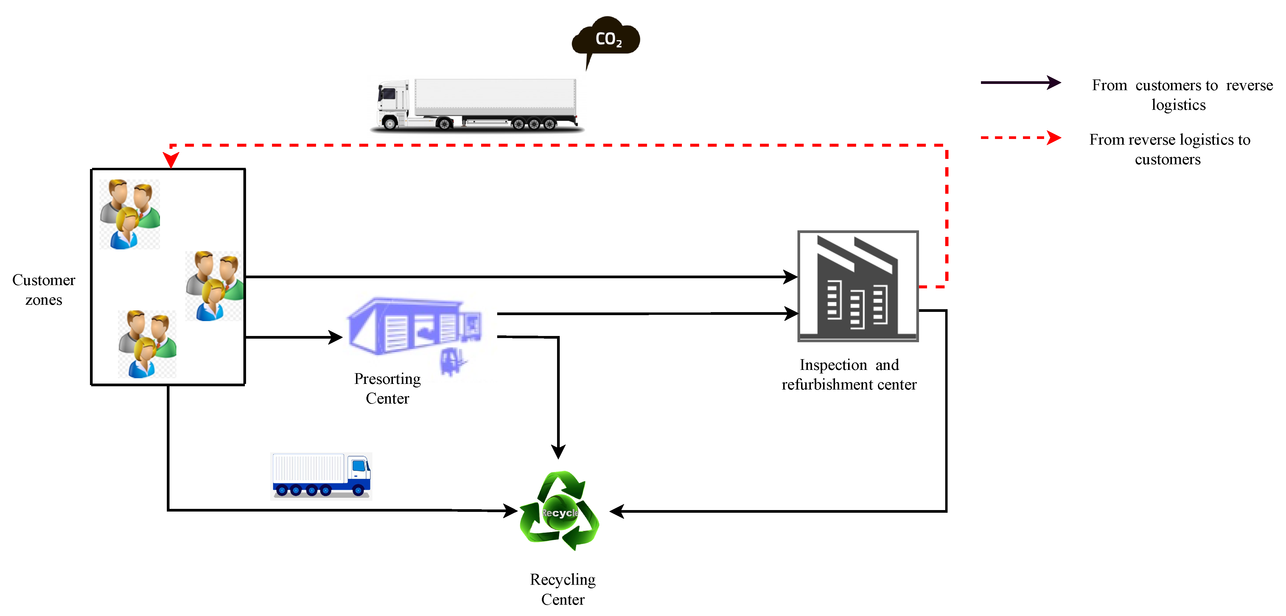
The GCLSC proposed in this study compromises a set of customer zones where the returned products are collected, a set of presorting centers located at these zones, a recycling center, and an inspection and refurbishment (IR) center with different capacity sizes: small, medium, and big. The structure of the proposed GCLSC network (Figure 2) is the same structure presented by Samuel et al. [20]. Transportation between the facilities is a heterogeneous transportation system comprising different vehicle fleets that are varied in capacity, cost, and carbon emissions. The returned products at customer zones are either subject to presorting or nonpresorting, depending on the quality of the returned products. For high or very low-quality products, it is obvious that they can be transferred directly to the IR and recycling centers, respectively. Otherwise, the returned products are presorted in the presorting center depending on the quality of these products and the efficiency of the presorting center. A fraction of these products are sent to the recycling center, and the rest are sent to the IR center.

To maximize the profit that results from the difference between the selling of refurbished products and the total cost incurred in the network and minimize the total carbon emissions due to processes and transportation activities in the network, we consider further assumptions as follows:

• The refurbished products are in a condition as good as new ones.
• Selling price, costs, and carbon emissions are subject to uncertainty with an unknown probability distribution.
• The capacities, costs, and carbon emissions due to transportation modes are predefined. Costs and emissions are based on the round trip distances between network facilities.
• The locations of customers zones, the recycling center, and the IR center are predefined.
• The capacities of the facilities are predefined and deterministic.
• Only one transportation mode can be used between any two consecutive facilities in the GCLSC network.

Based on the above assumptions and description, an MILP model of the proposed bi-objective GCLSC network and its nomenclature presented at the end of this paper.

On the one hand, the first objective function, ${\tilde{g}}_{pro}$, of the proposed model is the maximization of the profit; it comprises four parts: the first part, ${\tilde{g}}_1$, represents the selling price of the refurbished products at the IR center; the second part, ${\tilde{g}}_2$, represents the fixed costs of opening facilities in the entire network; the third part, ${\tilde{g}}_3$, represents the transportation costs due to transportation activities in the GCLSC network using heterogeneous modes of transportation of vehicles v; the last part, ${\tilde{g}}_4$, represents the cost of processing activities in the network, including presorting, inspection, refurbishment, and recycling.

On the other hand, the second objective function, ${\tilde{g}}_{emi}$, of the proposed model is the minimization of the carbon emissions due to the various activities in the GCLSC network; it comprises two parts: the first part, ${\widetilde{em}}_{tr}$, represents the emissions due to transportation activities using different modes of transportation vehicles in the network part of the objective function. The second part, ${\widetilde{em}}_{pr}$, is the emissions due to different processing activities in the network, such as presorting, inspection, refurbishing, and recycling.

$${\mathcal{P}}_{MOMILP}:\left\{\begin{array}{c}Max{\tilde{g}}_{pro}={\tilde{g}}_1-{\tilde{g}}_2-{\tilde{g}}_3-{\tilde{g}}_4\hfill \\ Min{\tilde{g}}_{emi}={\widetilde{em}}_{tr}+{\widetilde{em}}_{pr}\hfill \end{array}\right.$$

(1)

where

$${\tilde{g}}_1=\sum _{p\in P}\sum _{k\in K}\sum _{v\in V}{\tilde{s}}_{pk}{Z}_{pkv}^{ref}$$

(2)

$${\tilde{g}}_2=\sum _{s\in S}{\tilde{f}}_s{U}_s+\sum _{k\in K}{\tilde{f}}_k^p{U}_k+{\tilde{f}}_r{U}_r$$

(3)

$$\begin{array}{cc}\hfill {\tilde{g}}_3=& \sum _{p\in P}\sum _{k\in K}\sum _{v\in V}{\tilde{c}}_v^{tr}{w}_p{d}_{ki}{X}_{pkv}^{ins}+\sum _{p\in P}\sum _{k\in K}\sum _{v\in V}{\tilde{c}}_v^{tr}{w}_p{d}_{ki}{Y}_{pkv}^{ins}\hfill \\ & +\sum _{p\in P}\sum _{k\in K}\sum _{v\in V}{\tilde{c}}_v^{tr}{w}_p{d}_{ki}{Z}_{pkv}^{ref}+\sum _{p\in P}\sum _{v\in V}{\tilde{c}}_v^{tr}{w}_p{d}_{ir}{Z}_{pv}^{rec}\hfill \\ & +\sum _{p\in P}\sum _{k\in K}\sum _{v\in V}{\tilde{c}}_v^{tr}{w}_p{d}_{kr}{Y}_{pkv}^{rec}+\sum _{p\in P}\sum _{k\in K}\sum _{v\in V}{\tilde{c}}_v^{tr}{w}_p{d}_{kr}{X}_{pkv}^{rec}\hfill \end{array}$$

(4)

$$\begin{array}{cc}\hfill {\tilde{g}}_4=& \sum _{p\in P}\sum _{k\in K}{\tilde{p}}_{pk}^{pre}{X}_{pk}^{pre}+\sum _{p\in P}{\tilde{p}}_p^{ins}{G}_p^{ins}+\sum _{p\in P}\sum _{k\in K}\sum _{v\in V}{\tilde{p}}_p^{ref}{Z}_{pkv}^{ref}\hfill \\ & +\sum _{p\in P}\sum _{k\in K}\sum _{v\in V}{\tilde{p}}_p^{rec}{Y}_{pkv}^{rec}+\sum _{p\in P}\sum _{k\in K}\sum _{v\in V}{\tilde{p}}_p^{rec}{X}_{pkv}^{rec}+\sum _{p\in P}\sum _{v\in V}{\tilde{p}}_p^{rec}{Z}_{pv}^{rec}\hfill \end{array}$$

(5)

$$\begin{array}{cc}\hfill {\widetilde{em}}_{tr}=& \sum _{p\in P}\sum _{k\in K}\sum _{v\in V}{\widetilde{ev}}_v{w}_p{d}_{ki}{Y}_{pkv}^{ins}+\sum _{p\in P}\sum _{k\in K}\sum _{v\in V}{\widetilde{ev}}_v{w}_p{d}_{ki}{X}_{pkv}^{ins}\hfill \\ \hfill & +\sum _{p\in P}\sum _{k\in K}\sum _{v\in V}{\widetilde{ev}}_v{w}_p{d}_{ki}{Z}_{pkv}^{ref}+\sum _{p\in P}\sum _{v\in V}{\widetilde{ev}}_v{w}_p{d}_{ir}{Z}_{pv}^{rec}\hfill \\ \hfill & +\sum _{p\in P}\sum _{k\in K}\sum _{v\in V}{\widetilde{ev}}_v{w}_p{d}_{kr}{Y}_{pkv}^{rec}+\sum _{p\in P}\sum _{k\in K}\sum _{v\in V}{\widetilde{ev}}_v{w}_p{d}_{kr}{X}_{pkv}^{rec}\hfill & \\ \hfill & \hfill & \end{array}$$

(6)

$$\begin{array}{cc}\hfill {\widetilde{em}}_{pr}& =\sum _{p\in P}\sum _{k\in K}{\widetilde{em}}_p^{col}{r}_{pk}+\sum _{p\in P}\sum _{k\in K}{\widetilde{em}}_p^{pre}{X}_{pk}^{pre}+\sum _{p\in P}{\widetilde{em}}_p^{ins}{G}_p^{ins}+\hfill \\ \hfill & +\sum _{p\in P}\sum _{k\in K}\sum _{v\in V}{\widetilde{em}}_p^{ref}{Z}_{pkv}^{ref}+\sum _{p\in P}\sum _{k\in K}\sum _{v\in V}{\widetilde{em}}_p^{rec}{Y}_{pkv}^{rec}\hfill \\ \hfill & +\sum _{p\in P}\sum _{v\in V}{\widetilde{em}}_p^{rec}{Z}_{pv}^{rec}+\sum _{p\in P}\sum _{k\in K}\sum _{v\in V}{\widetilde{em}}_p^{rec}{X}_{pkv}^{rec}\hfill \end{array}$$

(7)

• Constraint (8) ensure the equilibrium at customer zone k; that is, the amount of returned product p equals the quantities sent to the recycling center for scrapping and IR center without presorting in addition to the amount sent for presorting centers.

  $$\sum _{v\in V}{X}_{pkv}^{ins}+X_{pk}^{pre}+\sum _{v\in V}{X}_{pkv}^{rec}=r_{pk}\forall p,k$$

  (8)
• Constraint (9) guarantees that the amount sent for presorting cannot exceed the amount of returned products.

  $$\sum _{p\in P}{X}_{pk}^{pre}\le U_k\sum _{p\in P}{r}_{pk}\forall k$$

  (9)
• Constraint (10) governs the quantity sent from the presorting center to the IR center, which comprises good-quality products and a fraction of bad-quality products due to the inefficiency of the presorting process.

  $$\sum _{v\in V}{Y}_{pkv}^{ins}=X_{pk}^{pre}\left(q_{pk}+\left(1-q_{pk}\right)\beta \right)\forall p,k$$

  (10)
• Constraint (11) guarantees that the amount sent from the customer zone k to the IR center of size s without presorting cannot exceed the maximum capacity of the biggest size of the IR center.

  $$\sum _{p\in P}\sum _{v\in V}{X}_{pkv}^{ins}\le c{a}^{big}\left(1-U_k\right)\forall k$$

  (11)
• Constraint (12) governs the quantity sent from the presorting center to the recycling center for scrapping.

  $$\sum _{v\in V}{Y}_{pkv}^{rec}=(1-\beta )\left(1-q_{pk}\right)X_{pk}^{pre}\forall p,k$$

  (12)
• Constraint (13) ensures that the presorted quantity is presorted is directed to the IR center or the recycling center for each product p and customer zone k.

  $$X_{pk}^{pre}=\sum _{v\in V}{Y}_{pkv}^{rec}+\sum _{v\in V}{Y}_{pkv}^{ins}\forall p,k$$

  (13)
• Constraint (14) governs the quantity of product p sent to the IR center from customer zone k, considering both presorted and non-presorted products. Constraint (15) guarantees the equilibrium at the IR center that the quantity of inspected product p is directed either for refurbishing or scrapping.

  $$G_p^{ins}=\sum _{k\in K}\sum _{v\in V}{Y}_{pkv}^{ins}+\sum _{k\in K}\sum _{v\in V}{X}_{pkv}^{ins}\forall p$$

  (14)

  $$G_p^{ins}=\sum _{k\in K}\sum _{v\in V}{Z}_{pkv}^{ref}+\sum _{v\in V}{Z}_{pv}^{rec}\forall p$$

  (15)
• Constraint (16) determines the quantity of a product p directed from the IR center to the recycling center; this quantity comprises a fraction due to the presorting center inefficiency, and the rest due to the bad quality of non-presorted products.

  $$\sum _{v\in V}{Z}_{pv}^{rec}=\sum _{k\in K}\sum _{v\in V}\left(1-q_{pk}\right)X_{pkv}^{ins}+\sum _{k\in K}\left(1-q_{pk}\right)\beta X_{pk}^{pre}\forall p$$

  (16)
• Constraint (17) stipulates that the quantity sent from the customer zones in the presence and absence of presorting in addition to the IR center to the recycling center cannot exceed its capacity.

  $$\sum _{v\in V}{X}_{pkv}^{rec}+\sum _{v\in V}{Y}_{pkv}^{rec}+\sum _{v\in V}{Z}_{pv}^{rec}\le c{a}_r{U}_r$$

  (17)
• Constraint (18) ensures that the total quantity of inspected products cannot exceed the capacity of the IR center of size s.

  $$\sum _{p\in P}{G}_p^{ins}\le c{a}_s{U}_s\forall s$$

  (18)
• Constraint (19) forces one size s of the IR center.

  $$\sum _{s\in S}{U}_s\le 1$$

  (19)
• Set of constraints with respect to multimode transportation vehicles v, constraints (20)–(25) ensure that only one type of vehicle is used to transport the products between every two facilities in the proposed GCLSC network.

  $$\sum _v{\dot{O}}_{kv}\le 1\forall k$$

  (20)

  $$\sum _v{O}_{kv}^{ref}\le 1\forall k$$

  (21)

  $$\sum _v{\dot{O}}_{kv}^{pre}\le 1\forall k$$

  (22)

  $$\sum _v{\ddot{O}}_{kv}\le 1\forall k$$

  (23)

  $$\sum _v{\ddot{O}}_{kv}^{pre}\le 1\forall k$$

  (24)

  $$\sum _v{\stackrel{⃛}{O}}_v\le 1$$

  (25)
• The set of constraints (26)–(31) guarantee that the quantity of transported products between two facilities cannot exceed the capacity of the total number of the vehicles of selected transportation mode v.

  $$\sum _{p\in P}{w}_p{X}_{pkv}^{ins}\le c{a}_v{\dot{N}}_{kv}\forall k,v$$

  (26)

  $$\sum _{p\in P}{w}_p{X}_{pkv}^{rec}\le c{a}_v{\ddot{N}}_{kv}\forall k,v$$

  (27)

  $$\sum _{p\in P}{w}_p{Y}_{pkv}^{ins}\le c{a}_v{\dot{N}}_{kv}^{pre}\forall k,v$$

  (28)

  $$\sum _{p\in P}{w}_p{Y}_{pkv}^{rec}\le c{a}_v{\ddot{N}}_{kv}^{pre}\forall k,v$$

  (29)

  $$\sum _{p\in P}{w}_p{Z}_{pkv}^{ref}\le c{a}_v{N}_{kv}^{ref}\forall k,v$$

  (30)

  $$\sum _{p\in P}{w}_p{Z}_{pv}^{rec}\le c{a}_v{\stackrel{⃛}{N}}_v\forall v$$

  (31)
• The set of constraints (32)–(37) that ensure the total number of vehicles of transportation mode v if this mode already has been selected.

  $${\dot{N}}_{kv}\le bigM{\dot{O}}_{kv}\forall k,v$$

  (32)

  $${\ddot{N}}_{kv}\le bigM{\ddot{O}}_{kv}\forall k,v$$

  (33)

  $${\dot{N}}_{kv}^{pre}\le bigM{\dot{O}}_{kv}^{pre}\forall k,v$$

  (34)

  $${\ddot{N}}_{kv}^{pre}\le bigM{\ddot{O}}_{kv}^{pre}\forall k,v$$

  (35)

  $$N_{kv}^{ref}\le bigM{O}_{kv}^{ref}\forall k,v$$

  (36)

  $${\stackrel{⃛}{N}}_v\le bigM{\stackrel{⃛}{O}}_v\forall v$$

  (37)
• The set of constraint (38) ensures that the total number of transported quantities between the facilities using the selected vehicle modes v equals the total number of returned products p.

  $$\begin{array}{cc}\hfill & \sum _{k\in K}\sum _{v\in V}c{a}_v{\dot{N}}_{kv}+\sum _{k\in K}\sum _{v\in V}c{a}_v{\ddot{N}}_{kv}+\sum _{k\in K}\sum _{v\in V}c{a}_v{\dot{N}}_{kv}^{pre}+\sum _{k\in K}\sum _{v\in V}c{a}_v{\ddot{N}}_{kv}^{pre}\hfill \\ & +\sum _{k\in K}\sum _{v\in V}c{a}_v{N}_{kv}^{ref}+\sum _{v\in V}c{a}_v{\stackrel{⃛}{N}}_v=\sum _{p\in P}\sum _{k\in K}{r}_{pk}\hfill \end{array}$$

  (38)
• Constraint (39) ensures that the carbon emissions due to transportation and processes activities cannot exceed the maximum allowable carbon emissions, that is, the carbon cap limit.

  $${\widetilde{em}}_{tr}+{\widetilde{em}}_{pr}\le {\widehat{c}}_{cap}$$

  (39)
• Constraints (40)–(42) represent the non-negativity, binary, and integrity constraints, respectively.

  $$Z_{pkv}^{ref}{G}_p^{ins},X_{pkv}^{rec},Y_{pkv}^{rec},Z_{pv}^{rec},X_{pk}^{pre},Y_{pkv}^{ins},X_{pkv}^{ins}\in {\mathbb{R}}_{\ge 0}$$

  (40)

  $$U_k,U_s,U_r,{\dot{O}}_{kv},{\dot{O}}_{kv}^{pre},{\ddot{O}}_{kv},{\ddot{O}}_{kv}^{pre},{\dot{O}}_{kv}^{ref},{\stackrel{⃛}{O}}_v\in \{0,1\}$$

  (41)

  $${\dot{N}}_{kv},{\ddot{N}}_{kv},{\dot{N}}_{kv}^{pre},{\ddot{N}}_{kv}^{pre},N_{kv}^{ref},{\stackrel{⃛}{N}}_v\in {\mathbb{Z}}^{\ast }$$

  (42)

4. The Robust Model of Bi-Objective Green Closed-Loop Supply Chain

RO is designed to deal with a lack of information. The uncertain parameters in robust optimization are taken at their worst case values; therefore, the robust optimization approach results in a solution that is immunized against uncertainty [24].

A general uncertain MILP model is given by

$$\begin{array}{c}\begin{array}{cc}\hfill \mathcal{P}:& \underset{x_j,y_k}{min}\sum _j{\tilde{c}}_j{x}_j+\sum _k{\tilde{e}}_k{y}_k\hfill \\ \hfill & \mathrm{s}.\mathrm{t}.\hfill \\ \hfill & \sum _j{\tilde{a}}_{ij}{x}_j+\sum _k{\tilde{b}}_{ik}{y}_k\le {\tilde{d}}_i\hfill & \hfill \forall i\in I\\ \hfill & x_j\in \mathbb{R}\hfill & \hfill \forall j\in J\\ & y_k\in \mathbb{Z}\hfill & \hfill \forall k\in K,\end{array}\end{array}$$

(43)

where $x_j$ and $y_k$ represent continuous and integer decision variables, respectively, ${\tilde{c}}_j$ and ${\tilde{e}}_k$ are the uncertain coefficients of the objective function, and ${\tilde{a}}_{ij}$, ${\tilde{b}}_{ik}$, and ${\tilde{d}}_i$ are the true values of the ith constraint coefficients that are subjected to uncertainty; the $\mathcal{P}$ model can be reformulated as follows:

$$\begin{array}{c}\begin{array}{cc}\hfill \mathcal{P}:& \underset{x_j,y_k,\beta }{min}\beta \hfill \\ \hfill & \mathrm{s}.\mathrm{t}.\hfill \\ \hfill & \sum _j{\tilde{c}}_j{x}_j+\sum _k{\tilde{e}}_k{y}_k\hfill & \hfill \le \beta & \\ \hfill & \sum _j{\tilde{a}}_{ij}{x}_j+\sum _k{\tilde{b}}_{ik}{y}_k\hfill & \hfill \le {\tilde{d}}_i& \forall i\in I\hfill \\ \hfill & x_j\in \mathbb{R}\hfill & \hfill & \forall j\in J\hfill \\ & y_k\in \mathbb{Z}\hfill & \hfill & \forall k\in K\hfill \end{array}\end{array}$$

(44)

Without loss of generality, we consider the general ith constraint, where the true value of uncertain constraint parameters ${\tilde{a}}_{ij}$, ${\tilde{b}}_{ik}$, and ${\tilde{d}}_i$ are $a_{ij}+{\widehat{a}}_{ij}{\xi }_{ij}$, $b_{ik}+{\widehat{b}}_{ik}{\xi }_{ik}$, and $d_i+{\widehat{d}}_i{\xi }_{i0}$, respectively; $a_{ij},b_{ik}$, and $d_i$ are the nominal value of the parameters, ${\widehat{a}}_{ij},{\widehat{b}}_{ik}$, and ${\widehat{d}}_i$ are the perturbations of the parameters around their nominal values respectively, and ${\xi }_{ij},{\xi }_{ik}$, and ${\xi }_{i0}$ are random independent variables that take values of $[-1,1]$. Hence, the ith constraint can be reformulated as follows:

$$\sum _{j\notin J_i}{a}_{ij}{x}_j+\sum _{j\in J_i}{\tilde{a}}_{ij}{x}_j+\sum _{k\notin K_i}{b}_{ik}{y}_k+\sum _{k\in K_i}{\tilde{b}}_{ik}{y}_k-{\widehat{d}}_i{\xi }_{i0}\le d_i$$

(45)

$J_i$ and $K_i$ are the sets that contain the uncertain parameters in the ith constraint. For simplicity, we consider $\xi =\{{\xi }_{ij},{\xi }_{ik},{\xi }_{i0}\}$ and U as the predefined set of random variables. To become immune against infeasibility that would result from any realization of uncertainty, the ith constraint can be rewritten as follows:

$$\begin{array}{cc}\hfill & \sum _j{a}_{ij}{x}_j+\sum _k{b}_{ik}{y}_k+\underset{\xi \in U}{max}\left\{\sum _{j\in J_i}{\xi }_{ij}{\widehat{a}}_{ij}{x}_j+\sum _{k\in K_i}{\xi }_{ik}{\widehat{b}}_{ik}{y}_k-{\widehat{d}}_i{\xi }_{i0}\right\}\le d_i\hfill \end{array}$$

(46)

The robust counterpart optimization formulation of the ith constraint based on the combined interval and polyhedral, “Interval + polyhedral” uncertainty set is as follows:

$$\left\{\begin{array}{c}\sum _j{a}_{ij}{x}_j+\sum _k{b}_{ik}{y}_k+\left[{\omega }_i\mathsf{\Gamma }+\sum _{j\in J_i}{\theta }_{ij}+\sum _{k\in K_i}{\eta }_{ik}+{\phi }_{i0}\right]\le d_i\hfill \\ {\omega }_i+{\theta }_{ij}\ge {\widehat{a}}_{ij}\left|x_j\right|\forall j\in J_i\hfill \\ {\omega }_i+{\eta }_{ik}\ge {\widehat{b}}_{ik}\left|y_k\right|\forall k\in K_i\hfill \\ {\omega }_i+{\phi }_{i0}\ge {\widehat{d}}_i\hfill \\ {\omega }_i,{\theta }_{ij},{\eta }_{ik},{\phi }_{i0}\ge 0\forall j\in J_i,\forall k\in K_i,\forall i\in I,\hfill \end{array}\right.$$

(47)

where ${\theta }_{ij},{\eta }_{ik},{\phi }_{i0}$, and ${\omega }_i$ are positive dual variables, and $\mathsf{\Gamma }$ represents the adjustable size parameter of the “Interval + Polyhedral” uncertainty set which reflects the degree of conservativeness. Figure 3 illustrates different geometrical representations of the combined “Interval + Polyhedral” uncertainty set based on the value of the adjustable parameter $\mathsf{\Gamma }$. The proof of robust counterpart formulation of the ith constraint, which is shown in Equation (47) is available in Li et al. [51] and Bertsimas and Sim [52].

Following the practical guide of the robust optimization approach proposed by Gorissen et al. [23] when the coefficients of the objective functions have uncertainty, constraints have been introduced to model the coefficients in the objective functions and approximate their values using auxiliary variables.

The robust counter reformulation of the ${\mathcal{P}}_{MOMILP}$ based on the “Interval + Polyhedral” uncertainty set induced an MILP model, ${\mathcal{RC}}_{I-P}-{\mathcal{P}}_{MOMILP}$, as follow:

$${\mathcal{RC}}_{I-P}-{\mathcal{P}}_{MOMILP}:\left\{\begin{array}{c}Max{\delta }_{pro}\hfill \\ Min{\delta }_{emi}\hfill \end{array}\right.$$

(48)

$$\left\{\begin{array}{ccc}\hfill & g_1-\hfill & \left[\sum _{p\in P_o}\sum _{k\in K_o}{\theta }_{pk}\right]-g_2-\left[\sum _{s\in S_o}{\theta }_s+\sum _{k\in K_o}{\theta }_k+{\theta }_r\right]-\hfill \\ \hfill & g_3-\hfill & \left[\sum _{v\in V_o}\left({\theta 1_v}^{ins}+{\theta 2_v}^{ins}+{\theta 3_v}^{ref}+{\theta 4_v}^{rec}+{\theta 5_v}^{rec}+{\theta 6_v}^{rec}\right)\right.-\hfill \\ \hfill & g_4-\hfill & \left[\sum _{p\in P_o}\sum _{k\in K_o}{{\theta }_{pk}}^{pre}+\sum _{p\in P_o}{{\theta }_p}^{ins}+\sum _{p\in P_o}{{\theta }_p}^{ref}\right.+\hfill \\ \hfill & \hfill & \sum _{p\in P_o}{\theta 1_p}^{rec}+\sum _{p\in P_o}{\theta 2_p}^{rec}+\left.\sum _{p\in P_o}{\theta 3_p}^{rec}\right]-{\mathsf{\Gamma }}_1{\omega }_1\ge {\delta }_{pro}\hfill \end{array}\right.$$

(49)

.

$$\begin{array}{cccc}{\omega }_1+{\theta }_{pk}\ge \hfill & {\widehat{s}}_{pk}{Z}_{pkv}^{ref}\hfill & \hfill & \forall p\in P,k\in K,v\in V\hfill \end{array}$$

(50)

$$\begin{array}{cccc}{\omega }_1+{\theta }_s\ge \hfill & {\widehat{f}}_s{U}_s\hfill & \hfill & \forall s\in S\hfill \end{array}$$

(51)

$$\begin{array}{cccc}{\omega }_1+{\theta }_k\ge \hfill & {\widehat{f}}_k^p{U}_k\hfill & \hfill & \forall k\in K\hfill \end{array}$$

(52)

$$\begin{array}{ccc}{\omega }_1+{\theta }_r\ge \hfill & {\widehat{f}}_r{U}_r\hfill & \hfill \end{array}$$

(53)

$$\begin{array}{cccc}{\omega }_1+\theta 1_v^{ins}\ge \hfill & {\widehat{c}}_v{X}_{pkv}^{ins}\hfill & \hfill & \forall p\in P,k\in K,v\in V\hfill \end{array}$$

(54)

$$\begin{array}{cccc}{\omega }_1+\theta 2_v^{ins}\ge \hfill & {\widehat{c}}_v{Y}_{pkv}^{ins}\hfill & \hfill & \forall p\in P,k\in K,v\in V\hfill \end{array}$$

(55)

$$\begin{array}{cccc}{\omega }_1+\theta 3_v^{ref}\ge \hfill & {\widehat{c}}_v{Z}_{pkv}^{ref}\hfill & \hfill & \forall p\in P,k\in K,v\in V\hfill \end{array}$$

(56)

$$\begin{array}{cccc}{\omega }_1+\theta 4_v^{rec}\ge \hfill & {\widehat{c}}_v{X}_{pkv}^{rec}\hfill & \hfill & \forall p\in P,k\in K,v\in V\hfill \end{array}$$

(57)

$$\begin{array}{cccc}{\omega }_1+\theta 5_v^{rec}\ge \hfill & {\widehat{c}}_v{Y}_{pkv}^{rec}\hfill & \hfill & \forall p\in P,k\in K,v\in V\hfill \end{array}$$

(58)

$$\begin{array}{cccc}{\omega }_1+\theta 6_v^{rec}\ge \hfill & {\widehat{c}}_v{Z}_{pv}^{rec}\hfill & \hfill & \forall p\in P,v\in V\hfill \end{array}$$

(59)

$$\begin{array}{ccc}{\omega }_1+{{\theta }_{pk}}^{pre}\ge {\widehat{p}}_{pk}^{pre}{X}_{pk}^{pre}\hfill & \hfill & \forall p\in P,k\in K\hfill \end{array}$$

(60)

$$\begin{array}{ccc}{\omega }_1+{{\theta }_p}^{ins}\ge {\widehat{p}}_p^{ins}{G}_p^{ins}\hfill & \hfill & \forall p\in P\hfill \end{array}$$

(61)

$$\begin{array}{ccc}{\omega }_1+{{\theta }_p}^{ref}\ge {\widehat{p}}_p^{ref}{Z}_{pkv}^{ref}\hfill & \hfill & \forall p\in P,k\in K\hfill \end{array}$$

(62)

$$\begin{array}{ccc}{\omega }_1+{\theta 1_p}^{rec}\ge {\widehat{p}}_p^{rec}{X}_{pkv}^{rec}\hfill & \hfill & \forall p\in P,k\in K\hfill \end{array}$$

(63)

$$\begin{array}{ccc}{\omega }_1+{\theta 2_p}^{rec}\ge {\widehat{p}}_p^{rec}{Y}_{pkv}^{rec}\hfill & \hfill & \forall p\in P,k\in K\hfill \end{array}$$

(64)

$$\begin{array}{ccc}{\omega }_1+{\theta 3_p}^{rec}\ge {\widehat{p}}_p^{rec}{Z}_{pv}^{rec}\hfill & \hfill & \forall p\in P,v\in V\hfill \end{array}$$

(65)

$$\left\{\begin{array}{cc}\hfill & {em}_{tr}+\left[\sum _{v\in V_o}\left(\eta 1_v^{ins}+\eta 2_v^{ins}+\eta 3_v^{ref}+\eta 4_v^{rec}+\eta 5_v^{rec}+\eta 6_v^{rec}\right)\right]\hfill \\ \hfill & {em}_{pr}+\left[\sum _{p\in P_o}\left(\eta 1_p^{col}+\eta 2_p^{pre}+\eta 3_p^{ins}+\eta 4_p^{ref}+\eta 5_p^{rec}+\eta 6_p^{rec}+\eta 7_p^{rec}\right)\right.+\hfill \\ \hfill & {\mathsf{\Gamma }}_2{\omega }_2\le {\delta }_{\mathit{emi}}\hfill \end{array}\right.$$

(66)

.

$$\begin{array}{cccc}{\omega }_2+\eta 1_v^{ins}\ge \hfill & {\widehat{ev}}_v{X}_{pkv}^{ins}\hfill & \hfill & \forall p\in P,k\in K,v\in V\hfill \end{array}$$

(67)

$$\begin{array}{cccc}{\omega }_2+\eta 2_v^{ins}\ge \hfill & {\widehat{ev}}_v{Y}_{pkv}^{ins}\hfill & \hfill & \forall p\in P,k\in K,v\in V\hfill \end{array}$$

(68)

$$\begin{array}{cccc}{\omega }_2+\eta 3_v^{ref}\ge \hfill & {\widehat{ev}}_v{Z}_{pkv}^{ref}\hfill & \hfill & \forall p\in P,k\in K,v\in V\hfill \end{array}$$

(69)

$$\begin{array}{cccc}{\omega }_2+\eta 4_v^{rec}\ge \hfill & {\widehat{ev}}_v{X}_{pkv}^{rec}\hfill & \hfill & \forall p\in P,k\in K,v\in V\hfill \end{array}$$

(70)

$$\begin{array}{cccc}{\omega }_2+\eta 5_v^{rec}\ge \hfill & {\widehat{ev}}_v{Y}_{pkv}^{rec}\hfill & \hfill & \forall p\in P,k\in K,v\in V\hfill \end{array}$$

(71)

$$\begin{array}{cccc}{\omega }_2+\eta 6_v^{rec}\ge \hfill & {\widehat{ev}}_v{Z}_{pv}^{rec}\hfill & \hfill & \forall p\in P,v\in V\hfill \end{array}$$

(72)

$$\begin{array}{cccc}{\omega }_2+\eta 1_p^{col}\ge \hfill & {\widehat{em}}_p^{col}{r}_{pk}\hfill & \hfill & \forall p\in P,k\in K\hfill \end{array}$$

(73)

$$\begin{array}{cccc}{\omega }_2+\eta 2_p^{pre}\ge \hfill & {\widehat{em}}_p^{pre}{X}_{pk}^{pre}\hfill & \hfill & \forall p\in P,k\in K\hfill \end{array}$$

(74)

$$\begin{array}{cccc}{\omega }_2+\eta 3_p^{ins}\ge \hfill & {\widehat{em}}_p^{ins}{G}_p^{ins}\hfill & \hfill & \forall p\in P,k\in K\hfill \end{array}$$

(75)

$$\begin{array}{cccc}{\omega }_2+\eta 4_p^{ref}\ge \hfill & {\widehat{em}}_p^{ref}{Z}_{pkv}^{ref}\hfill & \hfill & \forall p\in P,k\in K,v\in V\hfill \end{array}$$

(76)

$$\begin{array}{cccc}{\omega }_2+\eta 5_p^{rec}\ge \hfill & {\widehat{em}}_p^{rec}{X}_{pkv}^{rec}\hfill & \hfill & \forall p\in P,k\in K,v\in V\hfill \end{array}$$

(77)

$$\begin{array}{cccc}{\omega }_2+\eta 6_p^{rec}\ge \hfill & {\widehat{em}}_p^{rec}{Y}_{pkv}^{rec}\hfill & \hfill & \forall p\in P,k\in K,v\in V\hfill \end{array}$$

(78)

$$\begin{array}{cccc}{\omega }_2+\eta 7_p^{rec}\ge \hfill & {\widehat{em}}_p^{rec}{Z}_{pv}^{rec}\hfill & \hfill & \forall p\in P,v\in V\hfill \end{array}$$

(79)

and set of constraints that have been depicted in Equations (8)–(42).

The auxiliary variables, ${\delta }_{pro}$ and ${\delta }_{emi}$, are introduced to approximate the profit and carbon emissions, respectively. A set of constraints are presented in Equations (49)–(65) to model the robust counterpart of the first uncertain objective function ($Max{\tilde{g}}_{pro}^{}$).

A set of constraints are presented in Equations (66)–(79) to model the robust counterpart of the second uncertain objective function ($Min{\tilde{g}}_{emi}^{}$).

4.1. Probability Upper Bound of Constraint Violation in the Robust Optimization

In contrast to stochastic programming, RO does not require a known probability distribution to handle uncertain parameters. Probabilistic guarantees can be used to determine the lower bound on constraint satisfaction based on the desired constraint violation.

The probability upper bound of the constraint violation of the robust counterpart formulation based on the “Interval + Polyhedral” uncertainty set is proposed by Bertsimas and Sim [52] and Li et al. [53]. It is bounded $B\left(\left|Q_i\right|,\mathsf{\Gamma }\right)$, where $\left|Q_i\right|$ is the cardinality of the uncertain parameters in the ith constraint. Assuming the probability distribution of uncertainty is symmetric, independent, and bounded, it is given as follows:

$$\begin{array}{cc}\hfill & Pr\left\{\sum _j{a}_{ij}{x}_j+\sum _k{b}_{ik}{y}_k+\sum _{j\in J_i}{\xi }_{ij}{\widehat{a}}_{ij}{x}_j+\sum _{k\in K_i}{\xi }_{ik}{\widehat{b}}_{ik}{y}_k-{\widehat{d}}_i{\xi }_{i0}>d_i\right\}\hfill \\ & \le B\left(\left|Q_i\right|,\mathsf{\Gamma }\right)\hfill \end{array}$$

(80)

$$B\left(\left|Q_i\right|,\mathsf{\Gamma }\right)=\frac{1}{2^{\left|Q_i\right|}}\left\{(1-\mu )\sum _{l=\lfloor \nu \rfloor }^{\left|Q_i\right|}\left(\genfrac{}{}{0pt}{}{\left|Q_i\right|}{l}\right)+\mu \sum _{l=\lfloor v\rfloor +1}^{\left|Q_i\right|}\left(\genfrac{}{}{0pt}{}{\left|Q_i\right|}{l}\right)\right\}$$

(81)

where

$$v=\left(\left(\mathsf{\Gamma }+\left|Q_i\right|\right)/2\right),\mu =v-\lfloor v\rfloor .$$

• The proof of upper bounds on the probability of constraint violation is provided by Bertsimas and Sim [52] and Li et al. [53].

4.2. Solution Approach

Consider that $f\left(x\right)$ is a multi-objective model (MOM) with m objectives as $f\left(x\right)$$=\left\{f_1\left(x\right),f_2\left(x\right),\dots ,f_m\left(x\right)\right\}$. The general formulation of MOM is given below:

$$\begin{array}{c}Minf\left(x\right)\hfill \\ s.t.\hfill \\ x\in S\hfill \end{array}$$

(82)

Definition 1.

A decision vector ${\mathbf{x}}^{\ast }\in S$ is called Pareto optimal, or efficient, if there is no other decision vector $\mathbf{x}\in S$ such that $\mathbf{x}$ dominates ${\mathbf{x}}^{\ast }$. If ${\mathbf{x}}^{\ast }\in S$ is a Pareto optimal solution, the vector $\mathbf{f}\left({\mathbf{x}}^{\ast }\right)$ is said to be a non-dominated point in the objective space [54]. For instance, suppose that S⊂ ${\mathbb{R}}^3$ and its feasible region f⊂ ${\mathbb{R}}^2$, the continuous thick line contains all Pareto optimal solutions and $f\left(x^{\ast }\right)$ as one of these solutions (Figure 4).

Definition 2.

A decision vector ${\mathbf{x}}^{\ast }\in S$ is a weakly Pareto optimal, or weakly efficient, if there is no feasible solution $\mathbf{x}\in S$ such that $f\left(x\right)<f\left(x^{\ast }\right)$ is a weakly efficient solution, and the vector $f\left(x^{\ast }\right)$ is said to be a weakly non-dominated point in the objective space.

Definition 3.

A Pareto optimum solution is said to be supported if there are positive weights ${\lambda }_1,{\lambda }_2,\dots ,{\lambda }_k$ that make the solution optimal in terms of the linear combination (weighted sums problem): $min\left\{{\sum }_{i=1}^{i=k}{\lambda }_i{f}_i\left(x\right)\right\}$ s.t. $x\in S$ with coefficients ${\lambda }_1,{\lambda }_2,\dots ,{\lambda }_k$. If this is not the case, the solution is referred to be non-supported [55].

The solution approach implemented in this study is the LWT method which was developed by Steuer and Choo [56] to obtain Pareto optimal solutions by minimizing the maximum deviation of the objective functions from their values where they are optimized individually. The LWT approach outperforms existing techniques because of the following advantages [57,58]:

• Achieves adequate optimal solutions of MOMs.
• Provides both supported and non-supported Pareto solutions, whereas the weighted sum method, which is widely utilized in the literature, can only achieve supported Pareto solutions.
• Obtains Pareto optimal solutions in both the convex and concave space hulls.

The mathematical formulation of the LWT approach for MOM is given below:

$$\begin{array}{c}Min\alpha \hfill \\ s.t.\hfill \\ {\lambda }_i\left(f_i\left(x\right)-f_i^{\ast }\left(x^{\ast }\right)\right)\le \alpha \hfill \\ ⋮\hfill \\ {\lambda }_m\left(f_m\left(x\right)-f_m^{\ast }\left(x^{\ast }\right)\right)\le \alpha \hfill \\ \sum _{i=1}^m{\lambda }_i=1\hfill \\ 0\le {\lambda }_i\le 1\hfill \end{array}$$

(83)

The mathematical formulation of LWT approach for the robust counterpart model, ${RC}_{I-P}-{\mathcal{P}}_{MOMILP}$, of the bi-objective GCLSC based on the "Interval + Polyhedral" uncertainty set is as follows:

$$\begin{array}{cc}\hfill LWT-({\mathcal{RC}}_{I-P}-{\mathcal{P}}_{MOMILP})& :Min\alpha \hfill \\ \hfill & \mathrm{s}.\mathrm{t}\hfill \\ \hfill & {\lambda }_{\mathrm{pro}}\left({\delta }_{\mathrm{pro}}^{\ast }-{\delta }_{\mathrm{pro}}^{}\right)\hfill & \hfill \le \alpha \\ \hfill & {\lambda }_{\mathrm{emi}}\left({\delta }_{\mathrm{emi}}^{}-{\delta }_{\mathrm{emi}}^{\ast }\right)\hfill & \hfill \le \alpha \\ \hfill & {\lambda }_{\mathrm{pro}}+{\lambda }_{\mathrm{emi}}=1\hfill \\ \hfill & 0\le {\lambda }_{\mathrm{pro}},{\lambda }_{\mathrm{emi}}\le 1\hfill \end{array}$$

(84)

and set of constraints that have been depicted in Equations (8)–(42) and Equations (49)–(79).

5. Computational Experiments

In this section, to evaluate the performance of the proposed robust model of the GCLSC network by considering a presorting and heterogeneous transportation system using the LWT approach discussed in Section 4.2, a set of computational experiments was conducted using GAMS/CPLEX optimization solver. Most of the model input parameters were adopted from the literature [20], which are based on realistic data. Vehicle capacity and ${\mathrm{CO}}_2$ emissions were calculated for road transport operations as in Mohammed et al. [49], and the transportation cost based on vehicle type was calculated as in Wangsa and Wee [59] as shown in

Table 2. Cost, carbon emissions rate, and capacity of transportation modes.

	Cost (USD/kg-km)	${\mathbf{CO}}_2$$(\mathbf{g}/\mathbf{kg}\mathbf{km})$ Emissions	Vehicles Capacity (kg)
Light duty vehicles	0.00028	0.0000236	Uniform (0–4536)
Medium trucks	0.00014	0.0000452	Uniform (4537–11793)
Heavy duty trucks	0.00006	0.0000824	Uniform (11794–14969)

. The number of returned products, selling price of refurbished products at customer zones, operations costs, and weight of returned products are presented in

Table 3. Returned products, operations cost, and selling price of refurbished products.

	${\mathit{s}}_{\mathit{pk}}$			${\mathit{r}}_{\mathit{pk}}$			${\mathit{p}}_{\mathit{p}}^{\mathit{pre}}$	${\mathit{p}}_{\mathit{p}}^{\mathit{ref}}$	${\mathit{p}}_{\mathit{p}}^{\mathit{rec}}$	${\mathit{p}}_{\mathit{p}}^{\mathit{ins}}$	${\mathit{w}}_{\mathit{p}}$
	${\mathit{k}}_{\mathbf{1}}$	${\mathit{k}}_{\mathbf{2}}$	${\mathit{k}}_{\mathbf{3}}$	${\mathit{k}}_{\mathbf{1}}$	${\mathit{k}}_{\mathbf{2}}$	${\mathit{k}}_{\mathbf{3}}$
$p_1$	200	200	200	40,000	40,000	40,000	10	20	10	15	0.5
$p_2$	300	300	300	45,000	45,000	45,000	10	25	10	18	0.8
$p_3$	250	250	250	40,000	40,000	40,000	10	30	10	20	1.1

. Capacities and fixed opening costs of different sizes of the IR center are presented in

Table 4. Capacities and fixed opening costs of different IR center sizes.

	${\mathit{ca}}_{\mathit{s}}$	${\mathit{f}}_{\mathit{s}}$
Small	120,000	200,000
Medium	220,000	350,000
Big	300,000	500,000

. Distances between customer zones, the IR center, and the recycling center are presented in

Table 5. Distances between customer zones, the IR center, and the recycling center.

From∖To	IR Center	Recycling Center
$k_1$	100	200
$k_2$	150	300
$k_3$	200	400

, and the rest of the model parameters are presented in

Table 6. Rest of the model’s input parameters.

Parameter	Value
$e{m}_p^{col}$	0.03 kg CO${}_2$ per product
$e{m}_p^{pre}$	0.07 kg CO${}_2$ per product
$e{m}_p^{ins}$	0.09 kg CO${}_2$ per product
$e{m}_p^{ref}$	0.21 kg CO${}_2$ per product
$e{m}_p^{rec}$	0.07 kg $C{O}_2$ per product
${\widehat{c}}_{cap}$	120,000 kg CO${}_2$
$f_k^p$	USD 150,000
$f_r$	USD 250,000
$d_{ir}$	150 km
$c{a}_r$	30,000 units
$q_{pk}$	0.7
$\beta$	0.05

.

For model verification and to show the robustness of the RO approach, we consider that the perturbation of uncertain parameters are 5% and 10% around their nominal values assuming that the upper bounds of constraint violation are 10%, 15%, and 20%. In other words, the lower bounds of constraint satisfaction are 90%, 85%, and 80%, respectively. Five different weight sets (${\lambda }_{pro}$ and ${\lambda }_{emi}$) were considered for both the objective functions.

Increasing the lower bound of the probability of constraint satisfaction results in an increase in the conservative of the obtained solutions; that is, increasing the size of the uncertainty set $\mathsf{\Gamma }$ increases the costs that result in a decrease in the profit from the economic aspect. However, from the environmental perspective, increasing the uncertainty set leads to more carbon emission trade-offs between the conservatives and the values of profit and carbon emissions.

Robust objective function values were achieved at lower levels than the deterministic model. The values of the objective functions worsened as the perturbation around the nominal values increased (

Table 7. Robust Pareto front at 80% constraints satisfaction (5% perturbations).

${\mathit{\lambda }}_{\mathit{pro}}$	${\mathit{\lambda }}_{\mathit{emi}}$	Profit	Deviation	Carbon Emissions	Deviation
0.1	0.9	23,169,888	$-7$.29%	70,394	+1.10%
0.3	0.7	26,125,054	−7.28%	74,526	+1.09%
0.5	0.5	29,488,946	−6.60%	79,191	+1.10%
0.7	0.3	33,207,854	−6.09%	84,761	+1.34%
0.9	0.1	37,607,983	−5.24%	91,607	+1.52%

,

Table 8. Robust Pareto front at 80% constraints satisfaction (10% perturbations).

${\mathit{\lambda }}_{\mathit{pro}}$	${\mathit{\lambda }}_{\mathit{emi}}$	Profit	Deviation	Carbon Emissions	Deviation
0.1	0.9	21,346,559	−14.59%	71,162	+2.21%
0.3	0.7	24,190,076	−14.15%	75,283	+2.12%
0.5	0.5	27,335,999	−13.42%	80,122	+2.29%
0.7	0.3	31,043,425	−12.21%	85,910	+2.71%
0.9	0.1	35,530,213	−10.47%	93,000	+3.07%

,

Table 9. Robust Pareto front at 85% constraints satisfaction (5% perturbations).

${\mathit{\lambda }}_{\mathit{pro}}$	${\mathit{\lambda }}_{\mathit{emi}}$	Profit	Deviation	Carbon Emissions	Deviation
0.1	0.9	23,071,378	−7.69%	70,433	+1.16%
0.3	0.7	25,959,839	−7.86%	74,525	+1.09%
0.5	0.5	29,233,674	−7.41%	79,195	+1.10%
0.7	0.3	32,897,246	−6.97%	84,816	+1.40%
0.9	0.1	37,291,491	−6.03%	91,693	+1.62%

,

Table 10. Robust Pareto front at 85% constraints satisfaction (10% perturbations).

${\mathit{\lambda }}_{\mathit{pro}}$	${\mathit{\lambda }}_{\mathit{emi}}$	Profit	Deviation	Carbon Emissions	Deviation
0.1	0.9	21,137,593	$-15.42\%$	71,241	+2.32%
0.3	0.7	23,844,940	$-15.37\%$	75,287	+2.12%
0.5	0.5	26,866,979	$-14.91\%$	80,088	+2.24%
0.7	0.3	30,423,876	$-13.96\%$	86,015	+2.84%
0.9	0.1	34,897,458	$-12.07\%$	93,171	+3.26%

,

Table 11. Robust Pareto front at 90% constraints satisfaction (5% perturbations).

${\mathit{\lambda }}_{\mathit{pro}}$	${\mathit{\lambda }}_{\mathit{emi}}$	Profit	Deviation	Carbon Emissions	Deviation
0.1	0.9	22,977,737	$-8.06\%$	70,533	+1.30%
0.3	0.7	25,809,698	$-8.40\%$	74,611	+1.21%
0.5	0.5	29,045,184	$-8.01\%$	79,282	+1.21%
0.7	0.3	32,687,050	$-7.56\%$	84,920	+1.53%
0.9	0.1	37,076,867	$-6.57\%$	91,808	+1.74%

and

Table 12. Robust Pareto front at 90% constraints satisfaction (10% perturbations).

${\mathit{\lambda }}_{\mathit{pro}}$	${\mathit{\lambda }}_{\mathit{emi}}$	Profit	Deviation	Carbon Emissions	Deviation
0.1	0.9	20,930,083	$-16.25\%$	71,443	+2.61%
0.3	0.7	23,533,196	$-16.48\%$	75,462	+2.36%
0.5	0.5	26,525,935	$-15.99\%$	80,226	+2.42%
0.7	0.3	30,025,146	$-15.09\%$	86,169	+3.02%
0.9	0.1	34,465,757	$-13.15\%$	93,412	+3.52%

). On the one hand, when the perturbation was increased from 5% to 10%, for example, at a lower bound of the probability of constraint satisfaction of 80% and weights of ${\lambda }_{pro}$ = ${\lambda }_{emi}$ = 0.5, the profit declined by 6.62% and 13.42%, respectively, from their deterministic values. The value of carbon emissions, on the other hand, decreased by 1.10% and 2.29% from their deterministic levels, as shown in Table 7 and Table 8, respectively.

For the lower bound of constraint satisfaction at 80% with 5% data perturbations, the deviation of the robust profit decreased from its deterministic value by 5.24% to 7.29%. Meanwhile, the robust values of the carbon emission increase ranging from 1.09% to 1.52% (Table 7). By increasing the data perturbations to 10% the robust values for the profit and carbon emissions deviated by 10.47% to 14.59% and 2.12% to 3.07%, respectively (Table 8).

Increasing the lower bound of constraints satisfaction to 85% with 5% perturbations resulted in an increase in the deviation, ranging from 6.03% to 7.86% and 1.09% to 1.62% for the profit and carbon emissions, respectively, (Table 9). However, considering 10% perturbation, the deviation ranged from 12.07% to 15.42% and 2.12% to 3.26% for the profit and carbon emissions, respectively (Table 10).

For the lower bound of the probability of constraints satisfaction at 90% with 5% perturbation of the uncertain parameters, the deviation ranged from 6.57% to 8.40% and 1.21% to 1.74% for the profit and carbon emissions respectively (Table 11). In addition, considering 10% data perturbations, the deviation ranged from 13.15% to 16.25% and 2.61% to 3.52% for the profit and carbon emissions, respectively (Table 12).

Moreover, the robust optimal Pareto front of the bi-objective GCLSC model with 90% probability of constraints satisfaction with 5% and 10% is presented in Figure 5a,b, respectively. By increasing the deviation from the nominal values, the optimal values of the objective functions become worse as shown in the Pareto front representation in Figure 5.

On one hand, the obtained robust Pareto front of the proposed bi-objective GCLSC model is achieved with the levels of 80%, 85%, and 90% probability of constraints satisfaction and 5% and 10% of data perturbations, revealing that our model yields more conservative solutions that are immune against the uncertainty and comply with the nature of conflicting bi-objective functions.

On the other hand, increasing the probability of constraints satisfaction increases the uncertain space beside the integer variables of the model, hence increasing the model’s complexity.

6. Conclusions and Outlook

This study provided a robust bi-objective optimization model for the GCLSC network by considering a presorting and heterogeneous transportation system. The proposed bi-objective MILP model aims to maximize the profit and minimize the total carbon emissions incurred in the entire network by considering the selling price, costs, and carbon emissions uncertainties. A robust optimization approach based on the “Interval + Polyhedral” uncertainty set was adopted to tackle these uncertainties. An LWT approach was implemented to obtain the Pareto optimal solutions, which were hedges against perturbations of the uncertain parameters. A set of computational experiments was conducted to validate and show the performance of the proposed model.

Pareto optimal fronts of the robust bi-objective GCLSC model were examined considering the maximum probability of constraint violation. In other words, the lower bound of constraint satisfaction was considered at three levels: 80%, 85%, and 90% combined with 5% and 10% perturbations of the uncertain parameters around their nominal values. The lower the bound of constraint satisfaction, the more conservative as well as the less profit and more carbon emissions. Comparing the obtained robust solution with the deterministic solution in the experiments showed that our proposed model is more conservative and robust. Finally, the limitations of the proposed study, which can provide possible recommendations for future research, are as follows: the amount of time needed for computing is directly proportional to the number of integer variables; in other words, the amount of time needed for computation increases as the number of integer variables increases [60]. Small size instances are used in this paper for model validation. For large-scale problems, the model becomes computationally hard to obtain the optimal solution using the GAMS solver. Therefore, it is one of our future extension directions to propose heuristic or metaheuristic approaches to handle the large-size instances of the developed GCLSC.

However, future studies should extend the proposed robust bi-objective model to a multi-objective model by considering a social objective that contributes to the welfare and prosperity of society, such as maximizing the number of job opportunities and fair salaries for employees. Enhancement can be made using the quality of the robust solutions, the iterative solution framework proposed by Li and Floudas [61], and different uncertainty sets shapes such as ellipsoidal, polyhedral, combined “ellipsoidal and polyhedral”, and combined “box + ellipsoidal + polyhedral”.