Optimization of a Fuel Cost and Enrichment of Line Loadability for a Transmission System by Using Rapid Voltage Stability Index and Grey Wolf Algorithm Technique

Abstract

Efficient transmission of power is a pressing concern in modern power systems as it could relieve additional investments (e.g., right of way) and may improve stability. Non-uniform loading of transmission lines (which normally occurs due to the inefficient transmission of power) may lead to overloading of a few lines. These lines would then be prone to voltage instability. However, this problem would be aggravated under the network contingency condition. This paper focuses on improving the line loadability of the transmission system by considering the benchmark voltage stability index named rapid voltage stability index. The optimal loadability problem is considered using the grey wolf algorithm. The proposed work is implemented on a standard IEEE 30 bus test system using MATLAB software by addressing the problem by using line stability voltage index and grey wolf algorithm in optimal power flow. Minimizations of cost of generation, carbon emissions, voltage deviation, and line losses have been considered as objectives and improve the line loadability of the transmission system. The simulation results show that the proposed method is very effective in improving line loadability, reducing line congestion and fuel cost. Furthermore, the methodology is tested rigorously under various contingency conditions and is shown to be very effective. The proposed method relieves transmission line congestion and reduces fuel costs using the rapid voltage stability index (RVSI) is tested on an IEEE 30-bus standard test system utilizing MATLAB for various contingency lines

1. Introduction

Over the past few years, distribution generation has grown tremendously owing to fuel costs, carbon footprints, load requirement, delivers clean power, etc. Today, electrical system poses so many obstacles, including network connectivity, competition for loads, ecological imperatives, and the slender extension of the lines impacting worldwide management and efficiency. These problems pulled researchers through optimization techniques to make use of wind and solar generations to reduce transmission loss, fuel costs, and carbon discharges [1]. Those sources may be run either in isolated mode or grid-connected mode. The eccentric knowledge of wind and solar connected to traditional systems has given planners and analysts more difficulty in improving voltage stability, line flows, and sustainability. Optimal power flow was among the most popular innovations for power system design and optimization and will achieve enhanced operational status with the adaption of control variables to meet safe operations and physical constraints. It is appropriately tuned to decrease the real power loss, carbon emissions, generation cost, and maintains stability. Various optimization approaches for achieving the minimum values for particular systems have been explained [2].

The optimum power flow (OPF), which was developed some half a century ago, remains a broadly spoken topic in the power system research community. OPF’s main goal is to reduce various objective functions with the optimal setting of the control variables given by the data from the network. When minimizing the cost of generation, losses, emissions, etc., it is important to satisfy the network constraints on generator capacity, line capability, nodal voltages, and balanced power flow [3]. In many regions of the world, the development of renewable energy sources is being pursued to achieve the goal of producing sufficient electricity from renewable energy sources to meet the need for load requirements. Classical OPF consideration is taken as a concern when thermal generators operate on fossil fuels. With the growing penetration of solar and wind power into the grid, the OPF analysis has become essential to incorporate the uncertainties of solar and wind [4]. There are two categories of methods or approaches used for the optimization of OPF, namely deterministic and evolutionary approaches. Linear (LP) [5], nonlinear programming (NLP) [6], quadratic programming (QP) [7,8] and interior point method (IM) [9] are the deterministic methods. Because of the non-convexity of OPF concerns, those approaches have difficulty in handling most local minima. Gradient-based approaches overcome the problem of convergence, but sometimes inequality constraints are not met [6]. Evolutionary approaches were implemented to address this due to the drawbacks of deterministic methods. Several robust metaheuristics were evolved in recent decades. Some were impressively effective in solving the OPF issue are hybrid firefly-bat algorithm [10], moth swarm algorithm HAGOA [11], whale optimization algorithm [12], adaptive group search optimization [13], ant lion optimizer [14], differential evolution algorithm [15], modified bacteria foraging algorithm [16], backtracking search algorithm [17], particle swarm optimization [18]. The multi-objective grey wolf algorithm [19,20] is used to optimize power flow, voltage stability, line losses, and carbon emissions [21]. Fast under-frequency load shedding based on the GOA algorithm and compared to adaptive, PSO, and GA for various disturbances, with the objective function of minimizing the amount of load shed while optimizing the lowest swing frequency at different phases of the process being considered [22]. Developed a new model for mid-to-short-term load forecasting that can be used for different hours and days of the month. This method was tested for electricity purchase and production planning. This model combines the MTSTLF model with an MFFNN and the grasshopper optimization algorithm to produce highly accurate load forecasting results (GOA) [23]. developed and updated ANN training and forecasting methodology GA and MVO reduced the number of hidden layers, weights, and biases in ANNs. For various parameters, the MFFNN-MVO and MFFNN-GA models were compared for accuracy [24], used optimization techniques to maximize Savonius type wave turbine self-efficiency. The author also compared the WOA, AIS, BA, and PSO algorithms in maximizing the overall electrical output power from the wave turbine while constrained [25,26]. The power transfer capability of transmission networks is determined by the DG, societal well-being (weight 1), and network security (weight 2) weighting factors [27]. FPGA’s operational inaccuracies can be alleviated by combining the moth flame optimization (MFO) method with an artificial neural network (ANN) to improve forecasting accuracy for the suggested hybrid system.

The use of a few conventional and metaheuristic techniques for the optimization of the problem has been explained in this section. In general congestion and contingency causes the system to be voltage instability and overloading of the line subjected to the thermal load limit. To keep the system stable and operating in secured manner contingency conditions are also considered. When compared to the benchmark algorithms listed in Table 2, the proposed algorithm produces the best results globally.

A grey wolf algorithm influenced by nature, which provides improved solution and convergence functionality to boost network functioning relative to other methods, has been incorporated in this paper. The object of the paper is to demonstrate the proposed GWO algorithm is suitable for the issue of a power system to remove the overloads of line and stability problems while at the same time reducing, fuel production cost, voltage stability, and individual objective function. The viability of the suggested work with the IEEE 30 bus network has been proven. Minimizations of generation cost and line loss are considered as objectives and improve the line loadability of the transmission system. The proposed method relieves transmission line congestion and reduces fuel costs using rapid voltage stability index (RVSI) is examined on an IEEE 30-bus system for various contingency lines.

2. Problem Formulization

This study focuses on assessing the power system’s generation reallocation for normal and line contingency situations,

This might be written by:

MinimizeF(x,m):Subject to g(X,m) = 0, and h(X,m) < 0, X_l ≤ x ≤ X_u

(1)

F(x) defines scalar quantity, highlighting costs of fuel, carbon emissions, active power losses, and voltage deviations,

g(x) = equality constraint (that are the equations of power flow),

h(x) = inequality constraint (which refers to control parameter limits),

‘X’ refers to the state variable vector which comprises both controllable and dependent variables (i.e., generator bus voltages, reactive power generation, shunt converter voltages, line reactance, real power generation, series, and shunt susceptance).

‘m’ is a generator’s voltage, generators real power outputs, except for slack bus, in a vector of independent parameters, shunt Var compensators and tap setting of transformers, X_l and X_u are the lower and upper-value limits.

The solution process involves optimizing the objective function and meeting the constraints. Mathematically, this objective issue can be presented as below:

2.1. Objective Function

Total generation cost function can be minimized utilizing the associated quadratic Equation (1)

$$F_C(P_{TGI})={\displaystyle \sum _{i=1}^{N_{TG}}(a_i{P}_{TGI}^2+b_i{P}_{TGI}+C_i})\$/hr$$

(2)

where N_TG = no of thermal generator buses; a_i, b_i, c_i refers to the fuel cost coefficients of the ith unit; F_C = Net fuel cost function of thermal generators.

The cost of real power generation with the valve-point impact has been thought to be more operative and accurate in cost function modeling. When the influence of multi-valve turbines is taken into consideration, the power system’s cost of generation shows a greater range of variation and the sinusoidal function is updated to the cost of fuel.

$$F_{VPE}(P_{TG})={\displaystyle \sum _{i=1}^{N_{TG}}(a_i}{P}_{T_{GI}}^2+b_i{P}_{T_{GI}}+C_i+\left|d_i\times \sin (e_i\times (P_{T_{GI}}^{\min }-P_{T_{GI}}))\right|)$$

(3)

where d_i, e_i: Valve-point loading effect coefficients; $P_{TGI}^{\min }$: Minimum power of the ith thermal unit

This objective is comprised of the minimization of the real power losses of transmission lines. This can be represented as

$$F_{PL}=\min (P_{Loss})=\min ({\displaystyle \sum _{k=1}^{ntl}real(S_{ij}^k+S_{ji}^k)})$$

(4)

where ntl refers to the no. of transmission lines,

S_ij = net complex power flow of line ith bus–jth bus

The purpose of this deviation of voltage (VD) consideration is for the achievement of the needed voltage of transmission of a system may be stated by:

$$F_{VD}=\min (VD)=\min \left({\displaystyle \sum _{k=1}^{Nbus}|V_k-}{V}_k^{ref}|\right)$$

(5)

where V_k: voltage magnitude at bus k; V_k^ref: reference voltage magnitude at bus k.

With increasing the polluting environment, it is desirable to consider the carbon emission consideration to adjust the optimal flow of power. The net emissions ton/h of the pollutants from the thermal units may be expressed by

Carbon emissions are measured in tons per hour (ton/h) given as:

$$F_{CE}(P_{TGi})={\displaystyle \sum _{i=1}^{N_{TG}}[({\alpha }_i+{\beta }_i{P}_{TGi}+{\gamma }_i{P}_{TGI}^2)\times 0.01+{\omega }_i{e}^{({\mu }_i{P}_{TGi})}]}$$

(6)

where, α_i, β_i, γ_i, ω_i, µ_i: Emission coefficients of the ith thermal generator.

2.2. Equality Constraints

$$P_{Gi}-P_{Di}={\displaystyle \sum _{j=1}^N\left|V_i\right|}\left|V_j\right|\left|Y_{ij}\right|\cos ({\theta }_{ij}+{\delta }_j-{\delta }_i)$$

(7)

$$Q_{Gi}-Q_{Di}={\displaystyle \sum _{j=1}^N\left|V_i\right|}\left|V_j\right|\left|Y_{ij}\right|\sin ({\theta }_{ij}+{\delta }_j-{\delta }_i)$$

(8)

where P_Gi: active power generation; Q_Gi: reactive power generation; N: no. of. buses

2.3. Constraints Imposed by Inequality

(1)

Generator bus voltage restrictions:

$$V_{Gi}^{\min }\le V_{Gi}\le V_{Gi}^{\max }, G_i= 1, 2, 3\dots {\mathrm{n}}_{\mathrm{gb}}$$

(9)

(2)

Limits of real power generation:

$$P_{Gi}^{\min }\le P_{Gi}\le P_{Gi}^{\max }, G_i=1, 2, 3\dots {\mathrm{n}}_{\mathrm{gb}}$$

(10)

(3)

Reactive Power generated limits:

$$Q_{Gi}^{\min }\le Q_{Gi}\le Q_{Gi}^{\max }, G_i= 1, 2, 3\dots {\mathrm{n}}_{\mathrm{gb}}$$

(11)

n_gb is the No. of generator buses

(4)

Transmission line in MVA limit

$$S_l\le S_l^{\max },l=1‥\dots NL$$

(12)

NL = no. of transmission lines

Rapid Voltage Stability Index (RVSI)

An electrical network’s voltage stability can be determined by using this test method. It’s a sign of a system’s vulnerability and the potential for a voltage drop [21].

$$RVS{I}_{ij}=4\frac{X_{ij}}{V_i^2}(\frac{P_j^2}{Q_j}+Q_j)$$

(13)

where RVSI_ij: RVSI applicable for the line linked with buses i and j.; P_j: real power at receiving end bus; Q_j: receiving end bus reactive power; V_i: sending bus voltage; X_ij: reactance in between buses ith and jth.

The RVSI magnitude of a highly congested line is near to unity. As a result, RVSI values must be kept below unity to ensure system stability.

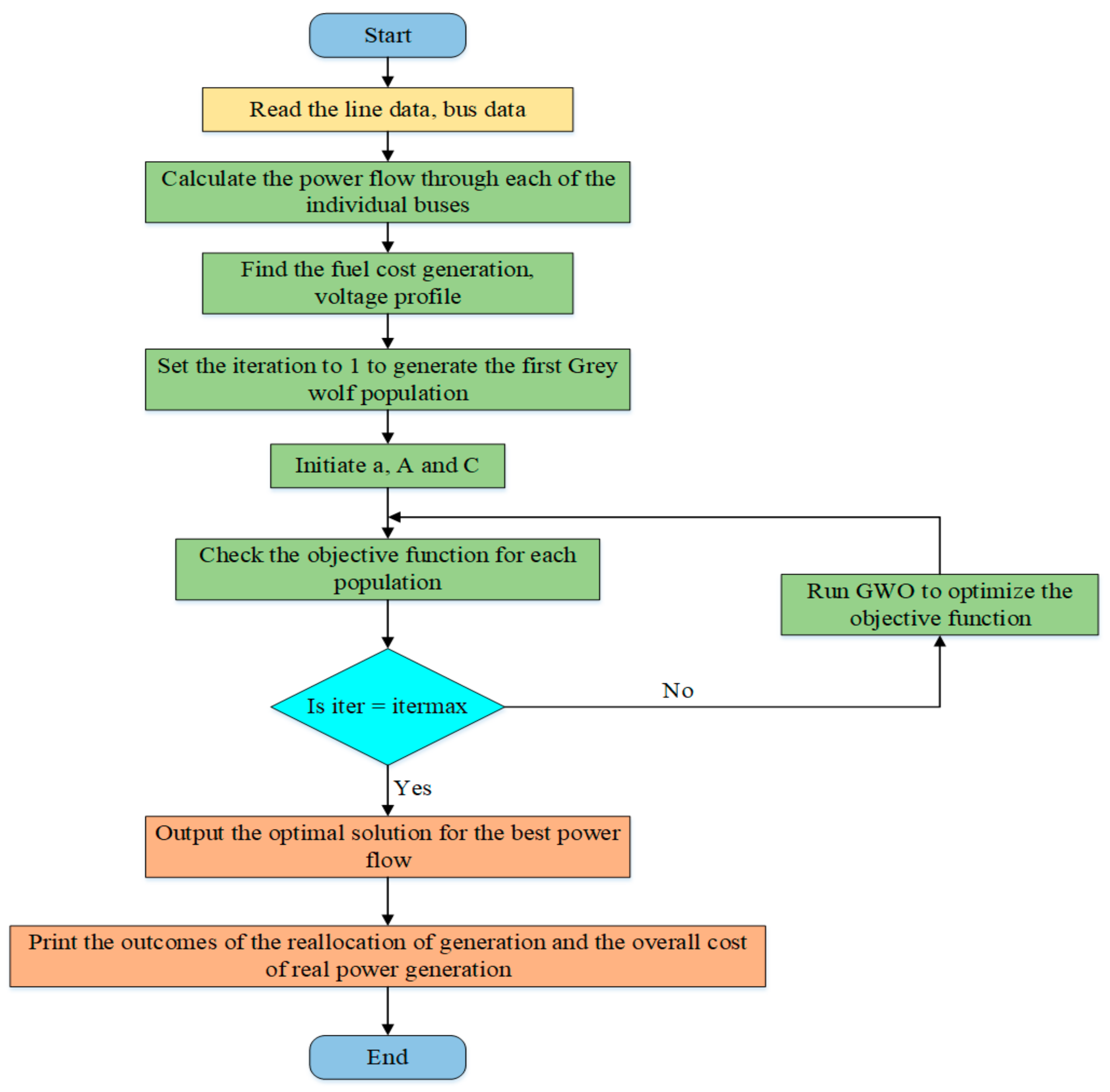
3. Proposed Grey Wolf Optimizer (GWO)

This optimizer was demonstrated in 2014 by Seyedalimirjalili and wasdesigned fully according to the hunt for grey wolves and individual characteristics for them. The author has acknowledged in this methodology four distinct aspects of hierarchical chains. Grey wolves such as ‘α’ come first, followed by ‘β’, ‘δ’, and finally ‘ω’. Grey wolves are becoming increasingly interested in remaining in a pack. The overall number of wolves in the pack could be between 5 and 12. ‘α’ wolves are typically the gathering chiefs, in charge of various actions such as fundamental leadership for chasing, strolling, attacking, relaxing, waking up, and so on. They do not need to be strong wolves but must deal with alternate wolves. In social situations, all grey wolves respect and recognize the pioneer wolf by holding their tails downwards. The ‘β’ grey wolf is the pack’s second leader, superior to the alternative wolves and the ‘α’ grey wolf. It could be either a female or a male. The ‘β’ wolf should supply the criticism obtained from the other wolves and assist the ‘α’ in making choices among different workouts conducted in the gathering. This wolf should lead the rest of the pioneer wolves. The next phase of the progressive system is ‘δ’ wolves, who are in charge of the lowest levels of the wolf hierarchy and show consideration for the more senior wolves. The remaining wolves are not very important; however, it has been observed that if one ‘δ’ wolf is loosed, the entire assembly fights. These are mostly in charge of the wolves’ gathering/minding, pack’s uprightness, and well-being [19]. A flow chart for an objective function utilizing the Grey Wolf approach is shown in Figure 1.

Algorithm for Grey Wolf Optimizer

Step 1: Establish GWO settings such as search agents (Ws), design variable size (Wd), and so on. the vectors a, A, and C, as well as the maximum no. of iterations

Ensure that the GWO’s search agents (Ws) and design variable sizes are set up (Wd). iterations and the number of vectors a, A, and C

A = 2.a.r₁ − a

(14)

C = 2.r₂

(15)

when component ‘a’ is linearly minimized from 2 to 0 throughout the iterations and r₁, r₂ are random vectors in [0,1].

Step 2: Build Grey wolves based on pack size arbitrarily. The grey wolves can be given as mathematically

$$Greywolves(W)\hspace{0.17em}=\hspace{0.17em}\hspace{0.17em}\left[\begin{array}{ccccc}{W}_{11}& W_{12}& \dots & W_{1n\_1}& W_{1n}\\ W_{21}& W_{22}& \dots & W_{2n\_1}& W_{2n}\\ .& .& \dots & .& .\\ W_{m\_11}& W_{m\_12}& \dots & W_{(m\_1)(n\_1)}& W_{(m\_1)n}\\ W_{m1}& W_{m2}& \dots & W_{(m)(n\_1)}& W_{mn}\end{array}\right]\hspace{0.17em}$$

where W_mn is the starting value of the mth pack of the nth wolves

Step 3: Estimate each hunting agent’s fitness value with the Formulas (16) and (17) below

$$D=\left|C\times \overrightarrow{W_p}(t)-\overrightarrow{W}(t)\right|$$

(16)

$$\overrightarrow{W}(t+1)=\overrightarrow{W_p}(t)-\overrightarrow{A}.\overrightarrow{D}$$

(17)

Step 4: Determine the best hunt agent (W_α), the second-best hunt agent(W_β) and the third-best hunt agent (W_δ) using equations

$$\begin{gathered} {\overrightarrow{D}}_{\alpha }=\left|{\overrightarrow{C}}_1\times {\overrightarrow{W}}_{\alpha }-\overrightarrow{W}\right| \\ {\overrightarrow{D}}_{\beta }=\left|{\overrightarrow{C}}_2\times {\overrightarrow{W}}_{\beta }-\overrightarrow{W}\right| \\ {\overrightarrow{D}}_{\delta }=\left|{\overrightarrow{C}}_3\times {\overrightarrow{W}}_{\delta }-\overrightarrow{W}\right| \\ {\overrightarrow{W}}_1=\left|{\overrightarrow{W}}_{\alpha }-{\overrightarrow{A}}_1\times {\overrightarrow{D}}_{\alpha }\right| \\ {\overrightarrow{W}}_2=\left|{\overrightarrow{W}}_{\beta }-{\overrightarrow{A}}_2\times {\overrightarrow{D}}_{\beta }\right| \\ {\overrightarrow{W}}_3=\left|{\overrightarrow{W}}_{\delta }-{\overrightarrow{A}}_3\times {\overrightarrow{D}}_{\delta }\right| \end{gathered}$$

Step 5: Renew the current hunting agent’s position using formula (18).

$$\overrightarrow{W}(t+1)=\frac{\overrightarrow{W_1}+\overrightarrow{W_2}+\overrightarrow{W_3}}{3}$$

(18)

Step 6: Estimate every hunt fitness value

Step 7: Updating the W_α, W_β, and W_δ values

Step 8: Find out what causes it to cease. In other words, if the number of iterations is reached, print the best solution value if possible, else return to s.

4. Results and Discussions

The load flow for the modified IEEE-30 bus system is considered and comprises of one slack bus, five thermal generators, the remaining are load buses and 41 interconnected lines. 100 MVA is chosen as the base MVA. Further, the system is tuned for optimal power flow by utilizing the grey wolf algorithm. In general, the thermal load limit restricts the power handling capability of a line. This limit is used for violation purposes and also severe contingencies which are causing security problems are also considered. Matlab 2015 with HP i5 Processor is used to generate the results for various objective functions and parameters. The parameters for the existing PSO and proposed grey wolf algorithm are shown in

Table 1. Parameters of PSO and GWO algorithm.

Parameters	PSO	GWO
Population size	20	20
Number of iterations	50	50
‘a’ vector	-	2
Cognitive constant c1	2	-
Social constant c2	2	-

.

Various objective functions, including losses, emissions, and fuel costs, are subjected to the Grey wolf algorithm under standard settings and compared to the existing methods. Figure 2 depicts a single-line diagram of the IEEE 30 bus system. These values are portrayed in

Table 2. The comparison of the suggested method with the optimal power flow.

Methods		Generation Fuel Cost ($/h)	Emission (ton/h)	Power Loss (MW)	The Influence of Valve Point on Fuel Cost ($/h)	Generation Fuel Cost (Rs/h)	The Influence of Valve Point on Fuel Cost (Rs/h)
Existing	MSFLA [28]	802.287	0.2056	-	-	59,056.3461	-
	SFLA [28]	802.509	0.2063	-	-	59,072.7022	-
	MDE [29]	802.376	-	-	-	59,062.8974	-
	IEP [30]	802.465	-	-	-	59,069.4487	-
	RGA [31]	-	--	4.5740	-	-	-
	CLPSO [32]	-	-	4.6282	-	-	-
	HSA [33]	-	-	4.9059	-	-	-
	PSO [34]	-	0.2063	5.1204	-	-	-
	IPSO [34]	-	0.2058	5.0732	-	-	-
Proposed	GWO	800.866	0.2041	4.229	828.2	58,951.7536	60,963.802

. It is also found that the various objective function values are reduced by incorporating the renewable energy sources and that the proposed algorithm is giving better results. It is considered one dollar is equal to 73.61 rupees for the calculations.

Figure 3 shows that in less than 50 iterations the objective functions smoothly convergences to the optimum value with no sudden changes in the objective function of fuel cost for normal conditions. The proposed GWO is shown to be effective in this way. Optimal control variable settings, objective fuel cost, and real power generation are shown in

Table 3. Comparison of control variables for different algorithms.

Control Variables	TS [35]	PSO	Proposed GWO
PG1 (MW)	176.04	179.9584	176.525
PG2 (MW)	48.76	50.7739	49.6202
PG5 (MW)	21.56	15.0000	21.9922
PG8 (MW)	22.05	22.8061	21.4111
PG11 (MW)	12.44	12.4457	10
PG13 (MW)	12	12	12
V1	1.05	1.06	1.06
V2	1.0389	1.0344	1.0353
V5	1.011	0.9857	0.9893
V8	1.0198	0.9826	0.9832
V11	1.0941	1.0820	1.082
V13	1.0898	0.9737	0.9743
Total real power generation (MW)	292.85	292.9840	292.5482
Total real power generation fuel cost ($/h)	802.29	802.6383	800.8661
Total real power generation fuel cost (Rs/h)	59,056.57	59,082.205	58,951.75

below. It is observed that Grey wolf optimization (GWO) has reduced the real power generation fuel cost as compared to the prevailing methods.

5. Contingency Management

The dynamic contingency management case was considered in this study. In such cases, two situations may occur. First of all, a line in the event of contingency can be considered to be extremely severe or a line in case of most contingencies can be most possibly severe. So, it can be classified as a probabilistic approach or deterministic approach. In this section, both methods were discussed and contrasted. The contingency ranking was given based on Rapid voltage stability severity index (RVSI) values for all lines in the descendant order of severity and can be obtained by removing all line outages. The maximum value of each line outage is identified and arranged these values in

Table 4. By using the traditional technique, severe lines for various line outages are listed in descending order of RVSI [36].

Line No	Line Outage		Severity Line		Line No	Line Outage		Severity Line
	SEB	REB	RVSI Max Value (p.u)	Line No with RVSI Max		SEB	REB	RVSI Max Value (p.u)	Line No with RVSI Max
5	2	5	0.594161	8	22	15	18	0.24757	13
9	6	7	0.364993	5	8	5	7	0.277803	5
2	1	3	0.319053	13	17	12	14	0.247424	13
4	3	4	0.314822	13	37	27	29	0.247378	13
14	9	10	0.296387	12	30	15	23	0.246917	13
6	2	6	0.282263	13	33	24	25	0.246853	13
15	4	12	0.276173	13	39	29	30	0.246657	13
7	4	6	0.276936	5	23	18	19	0.246584	13
36	28	27	0.265841	13	21	16	17	0.246553	13
3	2	4	0.257307	13	20	14	15	0.246357	13
41	6	28	0.252931	13	32	23	24	0.246193	13
12	6	10	0.252195	13	25	10	20	0.245787	13
18	12	15	0.251297	13	28	10	22	0.245764	13
10	6	8	0.250634	13	31	22	24	0.245764	13
35	25	27	0.249212	13	24	19	20	0.245552	13
19	12	16	0.248224	13	29	21	23	0.245403	13
38	27	30	0.247772	13	27	10	21	0.244637	13
40	8	28	0.247637	13	26	10	17	0.243553	13
-	-	-	-	-	11	6	9	0.241524	13

. These stability index values were obtained by running the Newton-Raphson method. These indices values can be used to signify the secure operating region of the system. A line closer to zero with RVSI is a good line for stability. The higher the magnitude of a line’s RVSI, the lower the stability line (i.e., closer it is to instability). From this Table 2 and Table 4, it is noted that for the line outage 2–5 the line between buses 5–7 (line number 8) with the RVSI value of 0.5941 is the maximum value and may be called severe. Line 2–5 is chosen as the most severe line from the deterministic approach for the analysis. In the probability approach most severe line between 9–11 buses (line no 13) is repeated more times for all line contingencies with a maximum value of RVSI 0.3190 for the line outage 1–3. The two-line outages (i.e., lines 3–4 and lines 4–12 and are considered for analysis).

Line flows were compared in different cases such as normal, normal with GWO, contingency with N-R load flow, and contingency with GWO in Table 4 for the IEEE 30 bus system. From this table, it could be noticed that the lines 1–2, 2–6, 4–6, 5–7 are overloaded under outage of lines 2–5. Congested lines are reduced to a significant value with the GWO method.

Table 5. Line outage contrast flows under the line 2–5.

SEB	REB	Power Flow Inline Limit (MVA)	Line Flows under Normal Condition	Line Flows with GWO	Line Flows under Line Outage	Line Flows under Line Outage with GWO
1	2	130	125.147	115.4587	132.9967	100.38
1	3	130	64.0504	64.0151	95.9061	79.0765
2	4	65	31.0057	34.8376	62.5328	56.1749
3	4	130	58.0709	59.0621	83.4757	72.0465
2	5	130	65.223	64.3444	----	-----
2	6	65	45.3089	49.0962	91.331	79.3818
4	6	90	52.6063	53.1096	99.6275	83.3106
5	7	70	14.1723	11.4026	71.761	67.8742
6	7	130	40.9623	34.072	123.0667	97.5358
6	8	32	26.9479	27.6367	27.3629	26.5946
6	9	65	11.3436	22.5704	10.3657	19.8392
6	10	32	11.9681	14.486	11.2084	13.2382
9	11	65	43.6356	36.6601	43.097	39.2178
9	10	65	47.8095	42.3696	46.285	42.8871
4	12	65	28.0796	32.8081	32.3194	34.4173
12	13	65	20.0104	12.0019	20.0144	12.0021
12	14	32	7.6908	7.409	8.1266	7.5954
12	15	32	17.475	16.9255	19.0046	17.5955
12	16	32	7.1029	7.0339	8.1706	7.4906
14	15	16	1.2331	1.29	1.588	1.4124
16	17	16	3.7012	4.1596	4.4319	4.4381
15	18	16	5.9792	5.9217	6.4918	6.1458
18	19	16	2.7471	2.7855	3.1601	2.9691
19	20	32	7.8197	8.0063	7.2553	7.778
10	20	32	10.3571	10.5182	9.8139	10.2932
10	17	32	8.9902	9.9232	7.7891	9.4894
10	21	32	24.5399	21.0537	23.7107	20.8295
10	22	32	7.9391	7.4723	8.0694	7.6786
21	23	32	3.6638	7.4253	2.8513	7.258
15	23	16	3.931	4.5358	5.0788	4.8863
22	24	16	7.8359	7.3875	7.9421	7.5841
23	24	16	2.9046	3.4657	3.3552	3.7389
24	25	16	1.0774	0.8738	1.1028	0.4273
25	26	16	4.2823	4.2728	4.304	4.2792
25	27	16	4.7819	4.8535	4.3359	4.3078
28	27	65	18.7488	19.0694	18.5246	18.5483
27	29	16	6.4588	6.4362	6.5136	6.4526
27	30	16	7.3424	7.315	7.4091	7.3348
29	30	16	3.7661	3.7599	3.7811	3.7644
8	28	32	4.7961	5.0108	4.4977	5.1228
6	28	32	15.0795	15.9036	15.2671	15.0442

described the Line outage contrast flows under the line 2–5. Line flows were compared in different cases such as normal, normal with GWO, contingency with N-R power flow, and contingency with GWO in

Table 6. The contrast of line flows under line outage of lines 3–4.

SEB	REB	Power Flow Inline Limit (MVA)	Line Flows under Normal Condition	Line Flows with GWO	Line Flows under Line Outage	Line Flows under Line Outage with GWO
1	2	130	125.147	115.4587	203.9089	170.6582
1	3	130	64.0504	64.0151	2.6344	2.6344
2	4	65	31.0057	34.8376	62.9633	60.5802
3	4	130	58.0709	59.0621	----	----
2	5	130	65.223	64.3444	77.8915	73.0946
2	6	65	45.3089	49.0962	71.6345	68.1407
4	6	90	52.6063	53.1096	24.6771	22.7873
5	7	70	14.1723	11.4026	9.5786	5.5252
6	7	130	40.9623	34.072	31.1187	26.7663
6	8	32	26.9479	27.6367	27.4867	26.4396
6	9	65	11.3436	22.5704	11.8525	21.3283
6	10	32	11.9681	14.486	12.8529	14.4471
9	11	65	43.6356	36.6601	43.087	39.1209
9	10	65	47.8095	42.3696	49.2146	44.9014
4	12	65	28.0796	32.8081	26.5851	29.0509
12	13	65	20.0104	12.0019	20.0154	13.4069
12	14	32	7.6908	7.409	7.4836	7.118
12	15	32	17.475	16.9255	16.6555	15.8252
12	16	32	7.1029	7.0339	6.4681	6.1998
14	15	16	1.2331	1.29	1.0241	1.0908
16	17	16	3.7012	4.1596	3.2596	3.6818
15	18	16	5.9792	5.9217	5.6681	5.4909
18	19	16	2.7471	2.7855	2.4704	2.4192
19	20	32	7.8197	8.0063	8.1475	8.4279
10	20	32	10.3571	10.5182	10.7698	10.9916
10	17	32	8.9902	9.9232	9.6481	10.6841
10	21	32	24.5399	21.0537	25.1893	21.9246
10	22	32	7.9391	7.4723	7.9373	7.6075
21	23	32	3.6638	7.4253	4.0898	7.8393
15	23	16	3.931	4.5358	3.2346	4.0189
22	24	16	7.8359	7.3875	7.8123	7.5125
23	24	16	2.9046	3.4657	2.6648	3.3656
24	25	16	1.0774	0.8738	1.1602	0.8808
25	26	16	4.2823	4.2728	4.3042	4.2807
25	27	16	4.7819	4.8535	5.0814	4.8782
28	27	65	18.7488	19.0694	19.4318	19.1998
27	29	16	6.4588	6.4362	6.5126	6.4558
27	30	16	7.3424	7.315	7.4078	7.3388
29	30	16	3.7661	3.7599	3.7809	3.7652
8	28	32	4.7961	5.0108	4.5103	5.2175
6	28	32	15.0795	15.9036	15.9832	15.4434

. From this table, it could be observed that lines 1–2, 2–6, are overloaded under the outage of lines 3–4. Congested lines are reduced to a significant value with the GWO method.

Line flows were compared in different cases such as normal, normal with GWO, contingency with N-R power flow, and contingency with GWO in

Table 7. The contrast of line flows under lines 4–12 outage.

SEB	REB	Power Flow Inline Limit (MVA)	Line Flows under Normal Condition	Line Flows with GWO	Line Flows under Line Outage	Line Flows under Line Outage with GWO
1	2	130	125.147	115.4587	130.7125	118.1491
1	3	130	64.0504	64.0151	64.6177	62.8055
2	4	65	31.0057	34.8376	29.6233	32.3256
3	4	130	58.0709	59.0621	58.4391	57.8071
2	5	130	65.223	64.3444	67.8305	66.7538
2	6	65	45.3089	49.0962	50.7587	53.7115
4	6	90	52.6063	53.1096	79.4628	81.2081
5	7	70	14.1723	11.4026	13.4958	10.6658
6	7	130	40.9623	34.072	38.8561	32.8465
6	8	32	26.9479	27.6367	27.8776	28.0066
6	9	65	11.3436	22.5704	24.6237	38.5999
6	10	32	11.9681	14.486	21.7286	25.2126
9	11	65	43.6356	36.6601	43.3637	38.1721
9	10	65	47.8095	42.3696	64.3463	61.0722
4	12	65	28.0796	32.8081	-------	------
12	13	65	20.0104	12.0019	20.0171	12.0027
12	14	32	7.6908	7.409	4.3573	3.3716
12	15	32	17.475	16.9255	6.9273	4.2853
12	16	32	7.1029	7.0339	5.2023	6.2669
14	15	16	1.2331	1.29	2.3298	3.12
16	17	16	3.7012	4.1596	8.4917	10.196
15	18	16	5.9792	5.9217	2.5957	1.4578
18	19	16	2.7471	2.7855	3.2718	3.7588
19	20	32	7.8197	8.0063	12.7137	13.7218
10	20	32	10.3571	10.5182	15.7133	16.6997
10	17	32	8.9902	9.9232	19.4694	21.5096
10	21	32	24.5399	21.0537	32.8053	30.8244
10	22	32	7.9391	7.4723	7.2653	7.0159
21	23	32	3.6638	7.4253	11.1083	14.6185
15	23	16	3.931	4.5358	8.1894	11.2538
22	24	16	7.8359	7.3875	7.1643	6.9306
23	24	16	2.9046	3.4657	0.9977	3.1415
24	25	16	1.0774	0.8738	4.7918	5.8736
25	26	16	4.2823	4.2728	4.2915	4.2783
25	27	16	4.7819	4.8535	9.1922	9.8949
28	27	65	18.7488	19.0694	24.0594	24.6506
27	29	16	6.4588	6.4362	6.4757	6.4458
27	30	16	7.3424	7.315	7.363	7.3267
29	30	16	3.7661	3.7599	3.7707	3.7625
8	28	32	4.7961	5.0108	4.8248	5.332
6	28	32	15.0795	15.9036	19.4053	20.2707

. From this table, it can be shown that the lines 1–2, 9–10, are overloaded under outage of lines 4–12. Congested lines are reduced to a significant value with the GWO method. The third column data Represents in Table 7 is the limit of power flows in the individual transmission line of the IEEE 30 Bus system. When these systems run using N-R Methos under normal conditions the fourth column shows the values of power flows in the individual line. column 5 of Table 7 shows the line flows in the individual transmission line by using the GWO algorithm. columns 7 and 8 show the line flows under line outage with and with the GWO algorithm as shown that the lines 1–2, 9–10, are overloaded under outage of lines 4–12. Congested lines are reduced to a significant value with the GWO method.

Table 8. Optimal power flows for various objective functions for various severe contingencies.

Parameters		Normal Case	Under Line Outage 3–4	Under Line Outage 2–5	Under Line Outage 4–12
Real power generation (MW)	PG1	177.525	169.3844	173.6528	175.3286
	PG2	49.6202	50.4766	50.872	48.1522
	PG5	21.9922	21.6592	26.5571	21.2868
	PG8	21.4111	26.3509	25.408	20.839
	PG11	10	13.7187	10	12.261
	PG13	12	13.4038	12	15.5942
Voltages in (P.U)	V1	1.06	1.06	1.06	1.06
	V2	1.0354	1.0133	1.0309	1.0325
	V5	0.9893	0.9585	0.8823	0.983
	V8	0.9833	0.9459	0.9495	0.9738
	V11	1.0602	1.0516	1.0571	1.0618
	V13	0.9744	0.9321	0.9451	0.8947
Performance parameters	Total generation of real power (MW)	292.5485	294.9936	298.4899	293.4618
	Total fuel cost for real power generation ($/h)	800.8612	812.2295	825.3745	805.1168
	Total fuel cost for real power generation (Rs/h)	58,951.39	59,788.213	60,755.82	59,264.65

shows over-loaded lines under various line outages. Power flows are observed in the line during normal conditions are within the specified limits but power flows line 2–6, line 1–2, line 5–7, line 4–6 gets congested due to the contingency of line 2–5. Power flows in lines 2–6, line 1–2, line 5–7, line 4–6 before contingency are 125.147 MVA, 45.3089 MVA, 52.6063 MVA, 14.1723 MVA, respectively. During contingency, the respective lines are overloaded to 132.996 MVA, 91.331 MVA, 99.62 MVA, 71.761 MVA, respectively, after using the proposed GWO these values are reduced to 100.38 MVA, 79.3818 MVA, 83.31 MVA, and 67.8742 MVA nearer to their limits. Similarly, this phenomenon was observed in the remaining line outages of lines 3–4, line 4–12.

Figure 4, Figure 5 and Figure 6 depicts the convergence characteristics of fuel cost function under the different contingency of line 2–5, line 3–4, line 4–12 using GWO approach from these figures it is observed that in less than 50 iterations the objective functions smoothly convergences to the optimum value with no sudden changes in the objective function of fuel cost for contingency conditions. This shows the efficiency of the proposed GWO compared with PSO.

Figure 7 displays the voltage profile of the generator as well as the load bus under normal and contingency conditions. Voltages are within limits during normal conditions and the voltage is disturbed during contingency and voltages are improved by using the proposed algorithm.

Table 9. Overloaded lines owing to contingency and their limits.

Line Outage	Congested Lines	Power Flow Limits in MVA	Line Flows under Normal Condition	Line Flow during Line Outage	Line Flow during Line Outage with GWO
2–5	1–2	130	125.147	132.996	100.38
	2–6	65	45.3089	91.331	79.3818
	4–6	90	52.6063	99.627	83.31
	5–7	70	14.1723	71.761	67.8742
3–4	1–2	130	125.147	203.9	170.6582
	2–6	65	45.3089	71.6345	68.1407
4–12	1–2	130	125.147	130.7125	118.1491
	9–10	65	47.8095	64.334	61.07

displays voltage magnitudes for various line outages.

Table 10. Voltage magnitudes for various line outages.

BUS N0	Normal Condition	Under Line Outage 3–4	Under Line Outage 2–5	Under Line Outage 4–12
V1	1.06	1.06	1.06	1.06
V2	1.0354	1.0133	1.0309	1.0325
V3	1.0136	1.0589	0.992	1.013
V4	1.0027	0.9594	0.9764	1.0019
V5	0.9893	0.9585	0.8823	0.983
V6	0.9955	0.958	0.9616	0.9864
V7	0.9893	0.9543	0.9237	0.9813
V8	0.9833	0.9459	0.9495	0.9738
V9	1.0093	0.9729	0.9786	0.9837
V10	0.9793	0.9406	0.9474	0.9441
V11	1.0602	1.0516	1.0571	1.0618
V12	0.9746	0.9323	0.9452	0.895
V13	0.9744	0.9321	0.9451	0.8947
V14	0.9628	0.9205	0.9327	0.8889
V15	0.9619	0.9203	0.931	0.8979
V16	0.9687	0.9276	0.9379	0.908
V17	0.9704	0.9307	0.9386	0.9274
V18	0.9549	0.9137	0.9232	0.9004
V19	0.9542	0.9134	0.9221	0.9054
V20	0.9596	0.9193	0.9275	0.9142
V21	0.9659	0.9261	0.9338	0.9247
V22	0.9682	0.9288	0.9357	0.9328
V23	0.9639	0.9239	0.9318	0.9209
V24	0.9532	0.913	0.92	0.9176
V25	0.9538	0.9138	0.9195	0.9297
V26	0.9349	0.894	0.8998	0.9103
V27	0.9634	0.9239	0.9287	0.9466
V28	0.989	0.9511	0.9549	0.9782
V29	0.9421	0.9016	0.9066	0.9249
V30	0.9299	0.8888	0.8938	0.9124

displays the many aspects of optimal control variables, objective functions such as losses, deviation of voltage, fuel cost with valve point influence, carbon emissions acquired values using the suggested algorithm.

From these results, it can be observed the lines are relieved from the overburden by utilizing the grey wolf algorithm. Therefore, most of the lines were relieved by using the proposed algorithm. Power generations for various line outages are shown in Figure 8.

6. Conclusions

The need for improved efficiency while ensuring system stability at the same time requires the development of enhanced approaches to system analysis and advanced technology advancement. Reallocation of maximum power generation is essential if system efficiency is to be improved using existing resources. Optimization techniques aim to get an optimal solution for the relocation of power generation. The critical contingencies that are causing problems for system security are taken into account.

The literature survey shows that the searching strategies influenced by evolution, including grey wolf and particle swarm algorithms, are suitable for approaching objective function. On IEEE 30-bus test systems the fitness, efficacy of the suggested algorithms has been tested. An essential objective of monitoring and taking the power system to the secure region has been accomplished. The outcomes of simulations show that each methodology has successfully achieved the goal of reducing various objective functions such as fuel cost, real power losses, carbon footprints, and voltage deviations. The GWO algorithm has also performed well in improving voltage stability and line load ability during overloads due to contingency by keeping the line capacity within thermal limits.

The future work can be extended by including various FACTS devices and by using the hybrid algorithm. The present work was considered for the constant load but can be extended by considering the variable loads

References

- Reddy, S.S.; Bijwe, P.R.; Abhyankar, A.R. Real-Time Economic Dispatch Considering Renewable Power Generation Variability and Uncertainty Over Scheduling Period. IEEE Syst. J. 2015, 9, 1440–1451. [Google Scholar] [CrossRef]
- Chen, G.; Qian, J.; Zhang, Z.; Sun, Z. Multi-objective Improved Bat Algorithm for optimizing fuel cost, emission and active power loss in power system. IAENG Int. J. Comput. Sci. 2019, 46, 118–133. [Google Scholar]
- Biswas, P.P.; Suganthan, P.; Amaratunga, G.A. Optimal power flow solutions incorporating stochastic wind and solar power. Energy Convers. Manag. 2017, 148, 1194–1207. [Google Scholar] [CrossRef]
- Rambabu, M.; Kumar, G.V.; Rao, B.V.; Kumar, B.S. Optimal power flow solution of an integrated power system using elephant herd optimization algorithm incorporating stochastic wind and solar power. Energy Sources Part A Recovery Util. Environ. Eff. 2021, 1–21. [Google Scholar] [CrossRef]
- Zehar, K.; Sayah, S. Optimal power flow with environmental constraint using a fast successive linear programming algorithm: Application to the algerian power system. Energy Convers. Manag. 2008, 49, 3362–3366. [Google Scholar] [CrossRef]
- Wei, H.; Sasaki, H.; Kubokawa, J.; Yokoyama, R. An interior point nonlinear programming for optimal power flow problems with a novel data structure. IEEE Trans. Power Syst. 1998, 13, 870–877. [Google Scholar] [CrossRef]
- Rambabu, M.; Kumar, G.V.N.; Sivanagaraju, S. Optimal Power Flow of Integrated Renewable Energy System using a Thyristor Controlled SeriesCompensator and a Grey-Wolf Algorithm. Energies 2019, 12, 2215. [Google Scholar] [CrossRef] [Green Version]
- Lavaei, J.; Rantzer, A.; Low, S. Power flow optimization using positive quadratic programming. IFAC Proc. Vol. 2011, 44, 10481–10486. [Google Scholar] [CrossRef] [Green Version]
- Capitanescu, F.; Glavic, M.; Ernst, D.; Wehenkel, L. Interior-point based algorithms for the solution of optimal power flow problems. Electr. Power Syst. Res. 2007, 77, 508–517. [Google Scholar] [CrossRef]
- Chen, G.; Qian, J.; Zhang, Z.; Sun, Z. Multi-Objective Optimal Power Flow Based on Hybrid Firefly-Bat Algorithm and Constraints-Prior Object-Fuzzy Sorting Strategy. IEEE Access 2019, 7, 139726–139745. [Google Scholar] [CrossRef]
- Dahiya, B.P.; Rani, S.; Singh, P. A Hybrid Artificial Grasshopper Optimization (HAGOA) Meta-Heuristic Approach: A Hybrid Optimizer for Discover the Global Optimum in Given Search Space. Int. J. Math. Eng. Manag. Sci. 2019, 4, 471–488. [Google Scholar] [CrossRef]
- Ben oualid Medani, K.; Sayah, S.; Bekrar, A. Whale optimization algorithm based optimal reactive power dispatch: A case study of the Algerian power system. Electr. Power Syst. Res. 2018, 163, 696–705. [Google Scholar] [CrossRef]
- Daryani, N.; Hagh, M.T.; Teimourzadeh, S. Adaptive group search optimization algorithm for multi-objective optimal power flow problem. Appl. Soft Comput. 2016, 38, 1012–1024. [Google Scholar] [CrossRef]
- Hatata, A.Y.; Lafi, A. Ant Lion Optimizer for Optimal Coordination of DOC Relays in Distribution Systems Containing DGs. IEEE Access 2018, 6, 72241–72252. [Google Scholar] [CrossRef]
- Reddy, S.S.; Bijwe, P.R. Differential evolution-based efficient multi-objective optimal power flow. Neural Comput. Appl. 2019, 31, 509–522. [Google Scholar] [CrossRef]
- Panda, A.; Tripathy, M. Security constrained optimal power flow solution of wind-thermal generation system using modified bacteria foraging algorithm. Energy 2015, 93, 816–827. [Google Scholar] [CrossRef]
- Shezan, S.A.; Ishraque, M.F. Assessment of a micro-grid hybrid wind-diesel-battery alternative energy system applicable for offshore islands. In Proceedings of the 2019 5th International Conference on Advances in Electrical Engineering (ICAEE), Dhaka, Bangladesh, 26–28 September 2019. [Google Scholar]
- Abido, M. Optimal power flow using particle swarm optimization. Int. J. Electr. Power Energy Syst. 2002, 24, 563–571. [Google Scholar] [CrossRef]
- Mirjalili, S.; Mirjalili, S.M.; Lewis, A. Grey Wolf Optimizer. Adv. Eng. Softw. 2014, 69, 46–61. [Google Scholar] [CrossRef] [Green Version]
- Nuvvula, R.; Devaraj, E.; Srinivasa, K.T. A Comprehensive Assessment of Large-scale Battery Integrated Hybrid Renewable Energy System to Improve Sustainability of a Smart City. Energy Sources Part A Recovery Util. Environ. Eff. 2021, 1–22. [Google Scholar] [CrossRef]
- Talaat, M.; Hatata, A.; Alsayyari, A.S.; Alblawi, A. A smart load management system based on the grasshopper optimization algorithm using the under-frequency load shedding approach. Energy 2020, 190, 116423. [Google Scholar] [CrossRef]
- Talaat, M.; Farahat, M.; Mansour, N.; Hatata, A. Load forecasting based on grasshopper optimization and a multilayer feed-forward neural network using regressive approach. Energy 2020, 196, 117087. [Google Scholar] [CrossRef]
- Talaat, M.; Said, T.; Essa, M.A.; Hatata, A.Y. Integrated MFFNN-MVO approach for PV solar power forecasting considering thermal effects and environmental conditions. Int. J. Electr. Power Energy Syst. 2022, 135, 107570. [Google Scholar] [CrossRef]
- Talaat, M.; Sedhom, B.E.; Hatata, A. A new approach for integrating wave energy to the grid by an efficient control system for maximum power based on different optimization techniques. Int. J. Electr. Power Energy Syst. 2021, 128, 106800. [Google Scholar] [CrossRef]
- Asija, D.; Choudekar, P. Power Transfer Loadability Enhancement of Congested Transmission Network Using DG. In Advances in Smart Communication and Imaging Systems; Lecture Notes in Electrical Engineering; Agrawal, R., Kishore Singh, C., Goyal, A., Eds.; Springer: Singapore, 2021; Volume 721. [Google Scholar] [CrossRef]
- Murty, V.; Kumar, A. Optimal placement of DG in radial distribution systems based on new voltage stability index under load growth. Int. J. Electr. Power Energy Syst. 2015, 69, 246–256. [Google Scholar] [CrossRef]
- Talaat, M.; Alblawi, A.; Tayseer, M.; Elkholy, M. FPGA control system technology for integrating the PV/wave/FC hybrid system using ANN optimized by MFO techniques. Sustain. Cities Soc. 2022, 80, 103825. [Google Scholar] [CrossRef]
- Shezan, S.A.; Hasan, K.N.; Datta, M. Optimal sizing of an islanded hybrid microgrid considering alternative dispatch strategies. In Proceedings of the 2019 29th Australasian Universities Power Engineering Conference (AUPEC), Nadi, Fiji, 26–29 November 2019. [Google Scholar]
- Sayah, S.; Zehar, K. Modified differential evolution algorithm for optimal power flow with non-smooth cost functions. Energy Convers. Manag. 2008, 49, 3036–3042. [Google Scholar] [CrossRef]
- Ongsakul, W.; Tantimaporn, T. Optimal Power Flow by Improved Evolutionary Programming. Electr. Power Compon. Syst. 2006, 34, 79–95. [Google Scholar] [CrossRef]
- Shezan, S.A. Feasibility analysis of an Islanded Hybrid Wind-Diesel-Battery Microgrid with Voltage and Power Response for Offshore Islands. J. Clean. Prod. 2020, 288, 125568. [Google Scholar] [CrossRef]
- Mahadevan, K.; Kannan, P. Comprehensive learning particle swarm optimization for reactive power dispatch. Appl. Soft Comput. 2010, 10, 641–652. [Google Scholar] [CrossRef]
- Khazali, A.; Kalantar, M. Optimal reactive power dispatch based on harmony search algorithm. Int. J. Electr. Power Energy Syst. 2011, 33, 684–692. [Google Scholar] [CrossRef]
- Niknam, T.; Narimani, M.; Aghaei, J.; Azizipanah-Abarghooee, R. Improved particle swarm optimisation for multi-objective optimal power flow considering the cost, loss, emission and voltage stability index. IET Gener. Transm. Distrib. 2012, 6, 515–527. [Google Scholar] [CrossRef]
- Ishraque, M.F.; Shezan, S.A.; Rashid, M.M.; Bhadra, A.B.; Hossain, M.A.; Chakrabortty, R.K.; Ryan, M.J.; Fahim, S.R.; Sarker, S.K.; Das, S.K. Techno-Economic and Power System Optimization of a Renewable Rich Islanded Microgrid considering different Dispatch Strategies. IEEE Access 2021, 9, 77325–77340. [Google Scholar] [CrossRef]
- Nuvvula, R.S.; Devaraj, E.; Elavarasan, R.M.; Taheri, S.I.; Irfan, M.; Teegala, K.S. Multi-objective mutation-enabled adaptive local attractor quantum behaved particle swarm optimisation based optimal sizing of hybrid renewable energy system for smart cities in India. Sustain. Energy Technol. Assess. 2022, 49, 101689. [Google Scholar] [CrossRef]