Active and Reactive Power Management in the Smart Distribution Network Enriched with Wind Turbines and Photovoltaic Systems

Abstract

The penetration of renewable energy sources has been intensified during the last decade to tackle the climate crisis by providing clean energy. Among various renewable energy technologies, wind turbines and photovoltaic systems have received increasing attention from investors. Generally, electronic power converters are used to control renewable generations. The present study discusses the power management of smart distribution networks enriched with wind and photovoltaic units. The model aims to minimize the expected network operating cost of the system formulated as an objective function regarding AC optimal power flow constraints. In addition, stochastic programming based on unscented transformation is adopted to model the probable behavior of loads, renewable generations, and energy market prices. The model employs a linear approximation model to burden the complexity of the problem and achieve the optimum solution. The problem is tested to a 33-bus system using the General Algebraic Modeling System (GAMS). The obtained results confirm the proposed model’s potential in reducing energy costs, power losses, and voltage deviations compared to conventional power flow studies. In the proposed scheme compared to network load distribution studies, the active and reactive power losses, network energy costs, and voltage deviations are improved by about 40.7%, 33%, 36%, and 74.7%, respectively.

1. Introduction

1.1. Motivation and Methodology

Due to the environmental effects of uncontrolled energy consumption, the application of green technologies has been increasing progressively in place of the conventional power plant as the main source of carbon emitters. The application of renewable energy sources (RESs), e.g., wind systems (WS) and photovoltaic systems (PVs), has been receiving significant attention to cope with both energy and climate change crises [1,2,3]. However, increasing the penetration of these resources in the distribution network without active management might cause power deviations in the system [4,5], leading to voltage deviations in some buses due to voltage upsurge and dips in buses [6]. Such problems generally occur due to incoordination and improper resource management, including active and reactive power generated by RESs. Considering the economic and environmental benefits of RESs, the network operator tends to fulfill customers’ energy requirements through these resources [7]. Although these resources are connected to the main grid via DC-AC and AC-AC converters equipped with the insulated-gate bipolar transistor (IGBT) bridge technologies [8], the growing development would lead to voltage deviation (overvoltage) [9]. Nonetheless, if the reactive power of nondispatchable elements is appropriately managed, the voltage profile can be controlled under the mentioned conditions. Thus, the proper management of active and reactive powers generated by RESs could improve the operating conditions of the distribution network [10,11].

In addition, operational problems typically have a low execution time; hence, these types of problems require low computational time [6,9]. To this aim, implementing a simple and linear model for the proposed network operation problem and modeling the uncertainties based on the methods with a low number of scenarios can achieve a low computational time [6]. Therefore, in order to achieve the mentioned goals (i.e., to improve the operation status and computational time of the network-connected RESs), simultaneous management of active and reactive power of smart distribution network using RES is conducted. In this design, it is assumed that DC-AC or AC-AC converters between the mentioned network resources are able to control both active and reactive power at the same time. Therefore, it is possible to obtain a favorable operation status in the distribution network by controlling them, especially in comparison with load flow studies [6,9]. In addition, linearization of the mentioned design and modeling uncertainties based on the Unscented Transformation method are appropriate ways for achieving low computational time.

1.2. Background

The exploitation of RESs in the distribution network has been studied in various works. So far, multiple studies have focused on deploying distributed generations (DG) in distribution systems. In [12], three reactive power control methods, including constant reactive power, constant power factor, and mixed methods, have been used to adjust the voltage profile. In [13], local voltage and reactive power control are provided by PVs. Ref. [14] examines the correlation between DGs and upstream networks using telecommunications. In this case, if a resource cannot modify the network indicators at the connection point, adjacent resources are used to deal with it. In [15], the optimal location of PVs is determined with the aim of minimizing network losses based on the daily load curve. The scheduling of a networked microgrid highly penetrated with RESs and mobile storage–electric vehicles (EVs) is discussed [16]. The model schedules resources in the day-ahead market and participates in real-time to minimize unbalances. The study adopts a two-layer energy management system (EMS) to manage microgrids, divided into single or aggregated microgrids. The first layer aims to minimize microgrids costs, while the second layer attempts to provide the minimum operating and risk costs. The model minimizes the day-ahead and real-time operational costs by adopting the second layer of the proposed EMS.

The application of EVs in a robust framework for optimal power management in distribution systems is utilized in [17], where energy costs are minimized concurrently. Furthermore, deterministic uncertainty sets are used to model uncertain parameters, including loads, EVs energy requirements, and EVs charger capacity and charging rates. The model adopts duality theory to turn the min-max model into a max model. The authors in [18] propose a robust optimization scheduling model to control the robustness level in an energy hub integrated with power-to-X technologies. An EMS is adopted [19] to reduce carbon emissions and costs associated with installations, repair, and operating costs of DGs and energy storage systems in an islanded hybrid system. The authors in [20] present an approach for the combined optimization of natural gas and electricity optimal power flow in a networked microgrid environment. Ref. [21] presents a novel EMS applied to a smart distribution system, where virtual power plants (VPPs) engage in energy and reserve markets. The profit of VPPs is maximized through the first layer of EMS, while the coordination of the VPP operator and power sources is handled in the second layer. The model can minimize the distribution system’s energy loss and voltage deviations by coordinating VPP and distribution system operators. The objective function is linearized and constrained by AC power flow equations. The authors in [20] propose an optimized operation model for energy hubs. To provide flexibility to energy hubs with RESs, various systems, including combined heat and power (CHP), storage, and incentive-based responsible load, are utilized. The objective function of the structured problem minimizes overall operating cost, as well as costs pertaining to reliability and flexibility services. The constraints consist of the AC power flow model and reliability levels in the energy hub system. The information-gap decision theory (IGDT) as a robust framework for an EMS is modeled in [22]. The hub operator manages the output electrical energy of the hub using RESs, storage system, and CHP. The authors in [22] present the optimal operation of microgrids containing DGs and thermal units by employing a novel EMS. The thermal load is supplied by CHP, boiler, and thermal storage systems. The model’s goal is to minimize three terms, comprising cost, energy loss, and voltage deviations. The paper adopts a multi-objective optimization approach and employs the ε-constraint technique to solve the problem.

1.3. Contributions

The literature review indicates that active power modeling is regarded in most power-related energy literature. Nonetheless, the control over active powers of nondispatchable resources is dismissed in literature since such resources are attractive to be deployed due to being eco-friendly with low operating costs. The increasing penetration of nondispatchable resources can adversely impact grid performance indicators such as voltage profiles. In most research, the use of energy storage devices along with renewable sources has been suggested to tackle the mentioned challenge. Storage devices store excess generations during off-peaks and inject them into the network in need. So, planning cost increases due to the installation cost of storage devices. The use of IGBT bridges in DC-AC or AC-AC converters could help overcome the problem by controlling the reactive power of these nondispatchable resources. Thus, the concurrent control over both active and reactive powers would improve the operating indicators effectively. On the other hand, renewable generations are highly dependent on external factors. Scenario-based stochastic modeling is commonly utilized to model the uncertain behavior of these resources, which is prone to high complexity.

Therefore, to address the research gaps, this paper manages the active and reactive power of the smart distribution network using renewable energy sources. This could reduce the negative effects of renewable resources in the network by controlling their reactive power. The proposed model also deals with various uncertainties, the modeling of which with scenario-based stochastic programming will increase the computational time of the problem. However, it should be noted that in the problems of power system operation, the executive step is generally small, so low computational time is of great importance in this type of problem [21,22]. It is considered as the next aim of the paper. It is, therefore, desirable that the method of uncertainty modeling generates a lower number of scenarios. Moreover, achieving simpler operating models such as its linearized model will be effective in reducing the computational time of the problem.

To overcome the obstacles mentioned above, this paper presents active-reactive power management of smart distribution networks (SDNs) penetrated with RESs, including WSs and PVs. The objective is to minimize the expected operating cost of the network, considering the technical constraints, e.g., the AC power flow and operating constraints of resources. Herein, the first-order Taylor series are employed to linearize power flow equations. In addition to this, the capacity constraints of resources, lines, and distribution substations, which are circular planes, are approximated to a regular polygon plane to achieve a linear model. The stochastic programming based on unscented transformation (UT) is employed to model the uncertainty of load, energy price market, WS, and PV active powers while mitigating the computational solving time of the problem. The novel contributions of the paper include:

• Simultaneous management of active and reactive power of smart distribution network using RESs to compensate for the adverse impacts of these resources in the network and improve network operational indicators,
• Modeling uncertainties of renewable power, energy prices, and load by UT approach to achieve the least number of scenarios and burden the problem’s computational complexity.
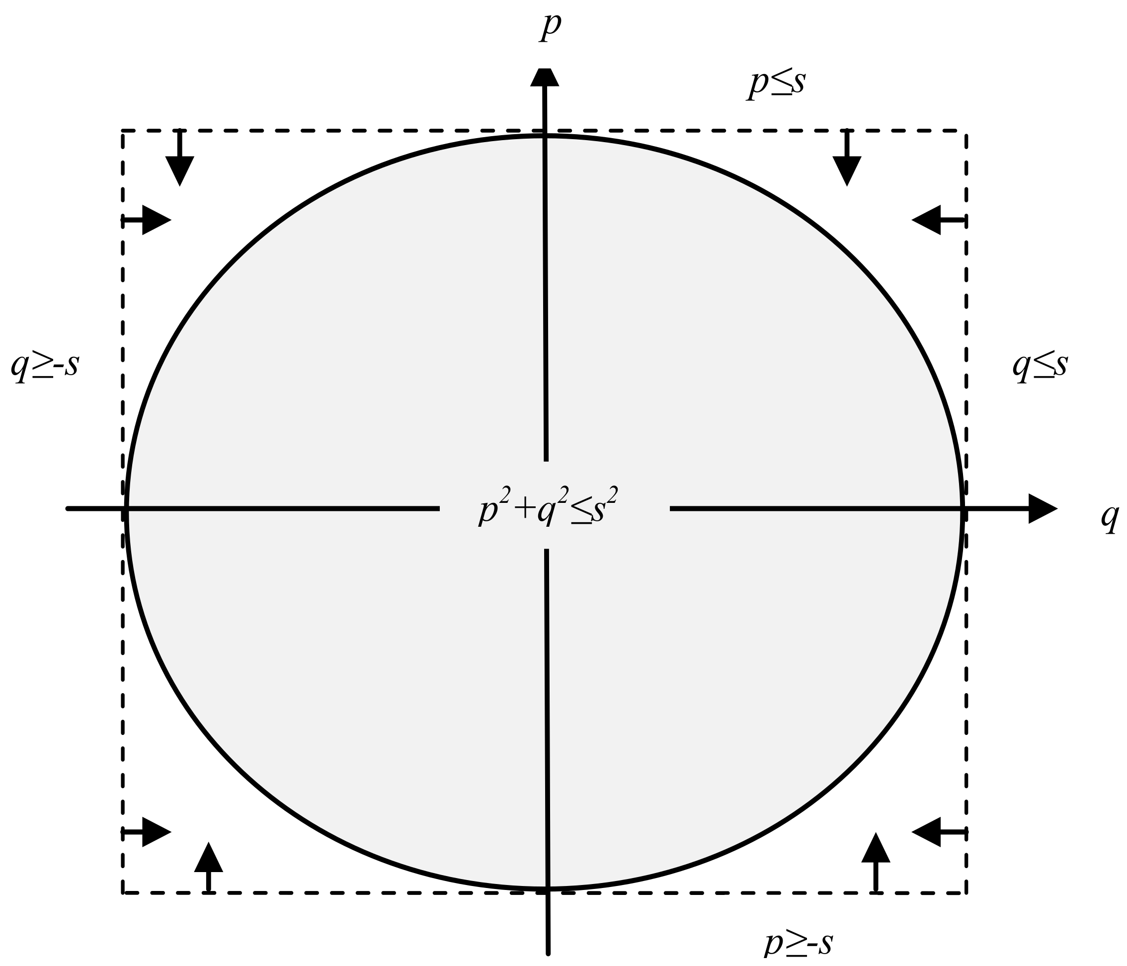
• Developing a linear approximation problem using the first-order Taylor series and approximating a circular plane to a regular polygon plane.

1.4. Paper Layouts

The layout of the paper is summarized as follows. Section 2 develops nonlinear and stochastic modeling of the proposed scheme. Section 3 describes the linear approximation model. Section 4 deals with numerical results, and conclusions are presented in Section 5.

2. Stochastic Scheduling of RESs in SDN

2.1. Power Management of RESs

The active and reactive power management problem of an SDN penetrated with renewable resources is modeled in this study. The objective is to minimize the expected energy cost regarding the technical network constraints as follows:

$$\min \hspace{1em}{\displaystyle \sum _{\varpi \in {\phi }_s}{\displaystyle \sum _{t\in {\phi }_t}{\pi }_{\varpi }{\lambda }_{o,\varpi }P{G}_{ref,o,\varpi }}}$$

(1)

Subject to:

$$P{G}_{i,o,\varpi }+P{W}_{i,o,\varpi }+P{V}_{i,o,\varpi }-P{D}_{i,o,\varpi }={\displaystyle \sum _{\kappa \in {\phi }_b}A{L}_{i,\kappa }P{L}_{i,\kappa ,o,\varpi }}\hspace{1em}\hspace{1em}\forall i,o,\varpi$$

(2)

$$Q{G}_{i,o,\varpi }+Q{W}_{i,o,\varpi }+Q{V}_{i,o,\varpi }-Q{D}_{i,o,\varpi }={\displaystyle \sum _{\kappa \in {\phi }_b}A{L}_{i,\kappa }Q{L}_{i,\kappa ,o,\varpi }}\hspace{1em}\hspace{1em}\forall i,o,\varpi$$

(3)

$$\begin{array}{l}P{L}_{i,\kappa ,o,\varpi }=g_{i,\kappa }{\left(V_{i,o,\varpi }\right)}^2-V_{i,o,\varpi }{V}_{\kappa ,o,\varpi }\cdot \\ \hspace{1em}\hspace{1em}\hspace{1em}\left\{g_{i,\kappa }\cos \left({\theta }_{i,o,\varpi }-{\theta }_{j,o,\varpi }\right)-b_{i,\kappa }\sin \left({\theta }_{i,o,\varpi }-{\theta }_{\kappa ,o,\varpi }\right)\right\}\hspace{1em}\hspace{1em}\forall i,\kappa ,o,\varpi \end{array}$$

(4)

$$\begin{array}{l}Q{L}_{i,\kappa ,o,\varpi }=-b_{i,\kappa }{\left(V_{i,o,\varpi }\right)}^2+V_{i,o,\varpi }{V}_{\kappa ,o,\varpi }\cdot \\ \hspace{1em}\hspace{1em}\hspace{1em}\left\{b_{i,\kappa }\cos \left({\theta }_{i,o,\varpi }-{\theta }_{j,o,\varpi }\right)+g_{i,\kappa }\sin \left({\theta }_{i,o,\varpi }-{\theta }_{\kappa ,o,\varpi }\right)\right\}\hspace{1em}\hspace{1em}\forall i,\kappa ,o,\varpi \end{array}$$

(5)

$${\theta }_{i,o,\varpi }=0\hspace{1em}\hspace{1em}\forall i=ref,o,\varpi$$

(6)

$$V_i^{\min }\le V_{i,o,\varpi }\le V_i^{\max }\hspace{1em}\hspace{1em}\forall i,o,\varpi$$

(7)

$${\left(P{L}_{i,\kappa ,o,\varpi }\right)}^2+{\left(Q{L}_{i,\kappa ,o,\varpi }\right)}^2\le {\left(S{L}_{i,\kappa }^{\max }\right)}^2\hspace{1em}\hspace{1em}\forall i,\kappa ,o,\varpi$$

(8)

$${\left(P{G}_{i,o,\varpi }\right)}^2+{\left(Q{G}_{i,o,\varpi }\right)}^2\le {\left(S{G}_i^{\max }\right)}^2\hspace{1em}\hspace{1em}\forall i=ref,o,\varpi$$

(9)

$$P{V}_{i,o,\varpi }=P{S}_{i,o,\varpi }+PL{V}_{i,o,\varpi }\hspace{1em}\hspace{1em}\forall i,o,\varpi$$

(10)

$$PL{V}_{i,o,\varpi }={\eta }_i^{pv}P{V}_{i,o,\varpi }+{\eta }_i^{qv}\left|Q{V}_{i,o,\varpi }\right|\hspace{1em}\hspace{1em}\forall i,o,\varpi$$

(11)

$${\left(P{V}_{i,o,\varpi }\right)}^2+{\left(Q{V}_{i,o,\varpi }\right)}^2\le {\left(S{V}_i^{\max }\right)}^2\hspace{1em}\hspace{1em}\forall i,o,\varpi$$

(12)

$$P{W}_{i,o,\varpi }=W_{i,o,\varpi }+PL{W}_{i,o,\varpi }\hspace{1em}\hspace{1em}\forall i,o,\varpi$$

(13)

$$PL{W}_{i,o,\varpi }={\eta }_i^{pw}P{W}_{i,o,\varpi }+{\eta }_i^{qw}\left|Q{W}_{i,o,\varpi }\right|\hspace{1em}\hspace{1em}\forall i,o,\varpi$$

(14)

$${\left(P{W}_{i,o,\varpi }\right)}^2+{\left(Q{W}_{i,o,\varpi }\right)}^2\le \left(S{W}_i^{\max }\right)\hspace{1em}\hspace{1em}\forall i,o,\varpi$$

(15)

Equation (1) describes the objective function of the problem aiming to minimize the expected network operating cost. The cost is the product of the power received from the network and the price of energy [23]. Equations (2)–(6) pertain to power flow equations [24,25,26,27,28], respectively, denoting the active and reactive power balances in each bus, the active and reactive power flow in each line, and the voltage angle of the reference bus. PG and QG represent the active and reactive power of the upstream network injected into the medium voltage (MV) distribution network. The distribution network is assumed to be interconnected to the upstream transmission network at the reference bus. Therefore, PG and QG have non-zero values for the reference bus and equate to zero for other buses. The voltage magnitude of the distribution network should be within its boundaries to prevent equipment insulation damage against overvoltage and network shut down against intense voltage drop as modeled in Equation (7). The branch flow limits of the distribution and transmission networks are formulated in Equations (8) and (9), respectively [29,30].

The operating model of RESs (WS and PV) are presented in (10)–(15). The PV output is modeled in Equation (10) while considering the power loss stemming from the DC-AC inverter unit as formulated in Equation (11). The apparent power of the PV unit needs to be within its boundaries as Equation (12). The same constraints are imposed on WS generations, as shown in Equations (13)–(15)

2.2. Uncertainty Modeling

In the problem described in Equation (1)–(15), active and reactive loads, renewable generations, energy prices are uncertain. Utilizing a Monte-Carlo simulation to model uncertain behavior of parameters might cause the model to be intractable [4,9]. Thus, the application of a UT approach can be effective in mitigating the complexity of such a large-scale problem [31]. The method generally uses the 2n + 1 model, where n represents the number of uncertainty parameters, and 2n + 1 represents the number of scenarios. Therefore, the number of extracted scenarios equals 11 in the proposed model, including five uncertain parameters. More specific details of the UT method can be fetched from [31].

Consider y = f(x) as the uncertain nonlinear stochastic problem, where y ∈ R^r indicates the vector of uncertain outputs containing r elements, and x ∈ Rⁿ denotes the vector of uncertain inputs with covariance and the mean values of σ_x and μ_x. The non-symmetrical entries provide the covariance of many uncertain variables, while the matrix σ_x symmetrical entries give the variance of uncertain parameters. The UT method is utilized for finding the mean and covariance output variables μ_y and σ_y [31]:

-

Step 1: 2n + 1 samples are taken from the input uncertain data:

$$x_0={\mu }_x$$

(16)

$$x_{\varpi }={\mu }_x+\sqrt{\frac{n}{1-W^0}{\sigma }_x}\hspace{0.17em}\hspace{0.17em}\hspace{0.17em}\hspace{0.17em}\hspace{0.17em}\hspace{0.17em}\hspace{0.17em}\forall \varpi =1,2,\mathrm{\dots },n$$

(17)

$$x_{\varpi }={\mu }_x-\sqrt{\frac{n}{1-W^0}{\sigma }_x}\hspace{0.17em}\hspace{0.17em}\hspace{0.17em}\hspace{0.17em}\hspace{0.17em}\hspace{0.17em}\hspace{0.17em}\forall \varpi =1,2,\dots ,n$$

(18)

In the above equations, W⁰ represents the weight of the mean value μ_x.

-

Step 2: The weighting coefficient of each sample point are evaluated:

$$W^0=W^0$$

(19)

$$W_{\varpi }=\frac{1-W^0}{2n}\hspace{0.17em}\hspace{0.17em}\hspace{0.17em}\hspace{0.17em}\hspace{0.17em}\hspace{0.17em}\hspace{0.17em}\forall \varpi =1,2,\dots ,n$$

(20)

$$W_{\varpi +n}=\frac{1-W^0}{2n}\hspace{0.17em}\hspace{0.17em}\hspace{0.17em}\hspace{0.17em}\hspace{0.17em}\hspace{0.17em}\hspace{0.17em}\forall \varpi +n=n+1,n+2,\dots ,2n$$

(21)

$${\displaystyle \sum _{\varpi =1}^n{W}_{\varpi }}=1$$

(22)

-

Step 3: 2n + 1 points are sampled to the nonlinear function to find output samples based on (23).

$$y_{\varpi }=f(x_{\varpi })$$

(23)

-

Step 4: The mean μ_y and covariance σ_y are evaluated values of the output variable ν:

$${\mu }_y={\displaystyle \sum _{\varpi =1}^n{W}_{\varpi }{\nu }_{\varpi }}$$

(24)

$${\sigma }_y={\displaystyle \sum _{\varpi =1}^n{W}_{\varpi }\left({\nu }_{\varpi }-{\mu }_y\right)}-{\left({\nu }_{\varpi }-{\mu }_y\right)}^T$$

(25)

3. Linear Model of the Scheme

As can be seen in the previous section, Equations (4), (6), (8), (9), (11), (12), (14) and (15) are nonlinear. In addition to the nonlinearities in the problem, Equations (4) and (5) are also non-convex. Hence, the model presented in the previous section is formulated as a non-convex nonlinear programming (NLP). Accordingly, considering the large scalability of the distribution network, the model would be intractable and cannot reach the optimal local solution due to the non-convex property of the problem [25,26,32]. It is also possible for meta-heuristic algorithms to reach the optimal solution in distribution networks, but the computational time would be high [33]. However, it should be noted that execution time is low in operational problems, so low computational time is of particular importance [21,22]. In addition, the proposed problem is non-convex, so different solvers obtain different solutions, and a unique solution could not be obtained [23,24]. Therefore, the current study develops a linear model of the proposed Section 2 problem to overcome the obstacle. Linear solvers can obtain a unique solution in low computational time. The linearization process is as follows.

3.1. Linear Formulation for Power Flow Model

Equations (4) and (5) are nonlinear. However, the following conditions are generally met in the distribution network:

• At the beginning and end of a distribution line, the voltage angle is less than 6° (0.105 rad) [34].
• The bus voltage magnitudes can be presumed 1 per unit (p.u.) if it varies from 0.9 to 1.05 p.u.

Given the above assumptions, the bus voltages can be written as 1 + ΔV, where ΔV is lower than 1. Moreover, $\cos ({\theta }_i-{\theta }_{\kappa })$ and $\sin ({\theta }_i-{\theta }_{\kappa })$ would be 1 and $({\theta }_i-{\theta }_{\kappa })$, respectively. The values of ΔV², $\Delta V\times ({\theta }_i-{\theta }_{\kappa })$, and $\Delta V_i\times \Delta V_{\kappa }$ are negligible, so they are disregarded in the model. Thus, Equations (4) and (5) are modified as Equations (26) and (27), respectively. Besides, the term “voltage deviation” is adopted in the model (28) so as to alter (7).

$$P{L}_{i,\kappa ,o,\varpi }=g_{i,\kappa }(\Delta V_{i,o,\varpi }-\Delta V_{\kappa ,o,\varpi })+b_{i,\kappa }({\theta }_{i,o,\varpi }-{\theta }_{\kappa ,o,\varpi })\hspace{1em}\hspace{1em}\forall i,\kappa ,o,\varpi$$

(26)

$$Q{L}_{i,\kappa ,o,\varpi }=-g_{i,\kappa }({\theta }_{i,o,\varpi }-{\theta }_{\kappa ,o,\varpi })-b_{i,\kappa }(\Delta V_{i,o,\varpi }-\Delta V_{\kappa ,o,\varpi })\hspace{0.17em}\hspace{0.17em}\hspace{0.17em}\hspace{0.17em}\forall i,\kappa ,o,\varpi$$

(27)

$$V_i^{\min }-1\le \Delta V_{i,o,\varpi }\le V_i^{\max }-1\hspace{1em}\hspace{1em}\forall i,o,\varpi$$

(28)

3.2. Linear Approximation of Circular Equations

As discussed above, Equations (8), (9), (12) and (15) are nonlinear. The equations represent the circle inequality, where the range of changes in active and reactive powers are within a circle with a radius of maximum apparent power. To determine the linear equations corresponding to the circular plane, Equation (29) is used as illustrated figuratively in Figure 1 [34,35]. Thus, a circular plane is developed by sharing several square planes. The linear expression of the circular plane is as (30) according to Figure 1.

$$p^2+q^2\le s^2$$

(29)

$$p\le s\hspace{0.17em}\hspace{0.17em},\hspace{0.17em}\hspace{0.17em}p\ge -s\hspace{0.17em}\hspace{0.17em},\hspace{0.17em}\hspace{0.17em}\hspace{0.17em}q\le s\hspace{0.17em}\hspace{0.17em}\&\hspace{0.17em}\hspace{0.17em}q\ge -s$$

(30)

According to Figure 1, Equation (30) is prone to a significant linearization error, which can be lessened by increasing the number of square plates with a different angle from the horizontal axis. Thus, the circle’s circumference is divided into equal parts (Δω), initially. The line equation is then calculated for each ς Δω, where ς represents the counter of the line segment. Eventually, the value of the Equation obtained for the line is less than or equal to the circle’s radius (s). In this case, the linear approximation equation related to the circular plane can be written as (31):

$$q\cos (\varsigma \times \Delta \omega )+p\sin (\varsigma \times \Delta \omega )\le s\hspace{1em}\hspace{1em}\varsigma \in {\phi }_{\varsigma }=\{0,1,\dots ,n_{\varsigma }-1\}$$

(31)

where $n_{\varsigma }$ is equal to the number of linear parts. For instance, if we use 180 square planes to linearize a circular plane, then $n_{\varsigma }$ is equal to 180 and Δω is 2°. In this case, the planes q ≤ s and p ≤ s correspond to ς = 0 and ς = 45, respectively. Thus, according to the above explanations, the linear approximations of Equations (8), (9), (12) and (15) are:

$$\cos (\varsigma \times \Delta \omega )\times P{L}_{i,\kappa ,o,\varpi }+\sin (\varsigma \times \Delta \omega )\times Q{L}_{i,\kappa ,o,\varpi }\le S{L}_{i,\kappa }^{\max }\hspace{1em}\hspace{1em}\forall i,\kappa ,o,\varpi ,\varsigma$$

(32)

$$\cos (\varsigma \times \Delta \omega )\times P{G}_{i,o,\varpi }+\sin (\varsigma \times \Delta \omega )\times Q{G}_{i,o,\varpi }\le S{G}_i^{\max }\hspace{1em}\hspace{1em}\forall i=ref,o,\varpi ,\varsigma$$

(33)

$$\cos (\varsigma \times \Delta \omega )\times P{V}_{i,o,\varpi }+\sin (\varsigma \times \Delta \omega )\times Q{V}_{i,o,\varpi }\le S{V}_i^{\max }\hspace{1em}\hspace{1em}\forall i,o,\varpi ,\varsigma$$

(34)

$$\cos (\varsigma \times \Delta \omega )\times P{W}_{i,o,\varpi }+\sin (\varsigma \times \Delta \omega )\times Q{W}_{i,o,\varpi }\le S{W}_i^{\max }\hspace{1em}\hspace{1em}\forall i,o,\varpi ,\varsigma$$

(35)

3.3. The Linear Correlation of the Losses Associated with Wind and Aggregated PV Units

Equations (11) and (14) are nonlinear due to the inclusion of the absolute magnitude of the reactive power of these elements. Regarding the reactive power part, the reactive power of the proposed systems is capacitive or negative owing to inductive loads. Thus, the linear model of Equations (11) and (14) will be reformulated as Equations (36) and (37). As discussed, the reactive power is negative, which has a direct impact on increasing the losses. Thus, the negative coefficient of the reactive power appears in the loss equations:

$$PL{V}_{i,o,\varpi }={\eta }_i^{pv}P{V}_{i,o,\varpi }-{\eta }_i^{qv}Q{V}_{i,o,\varpi }\hspace{1em}\hspace{1em}\forall i,o,\varpi$$

(36)

$$PL{W}_{i,o,\varpi }={\eta }_i^{pw}P{W}_{i,o,\varpi }-{\eta }_i^{qw}Q{W}_{i,o,\varpi }\hspace{1em}\hspace{1em}\forall i,o,\varpi$$

(37)

All in all, the proposed linear problem (LP) will be:

$$\min \hspace{1em}{\displaystyle \sum _{\varpi \in {\phi }_s}{\displaystyle \sum _{t\in {\phi }_t}{\pi }_{\varpi }{\lambda }_{o,\varpi }P{G}_{ref,o,\varpi }}}$$

(38)

Subject to:

Constraints (2), (3), (6), (10), (13), (26)–(28) and (32)–(37).

4. Numerical Results and Discussion

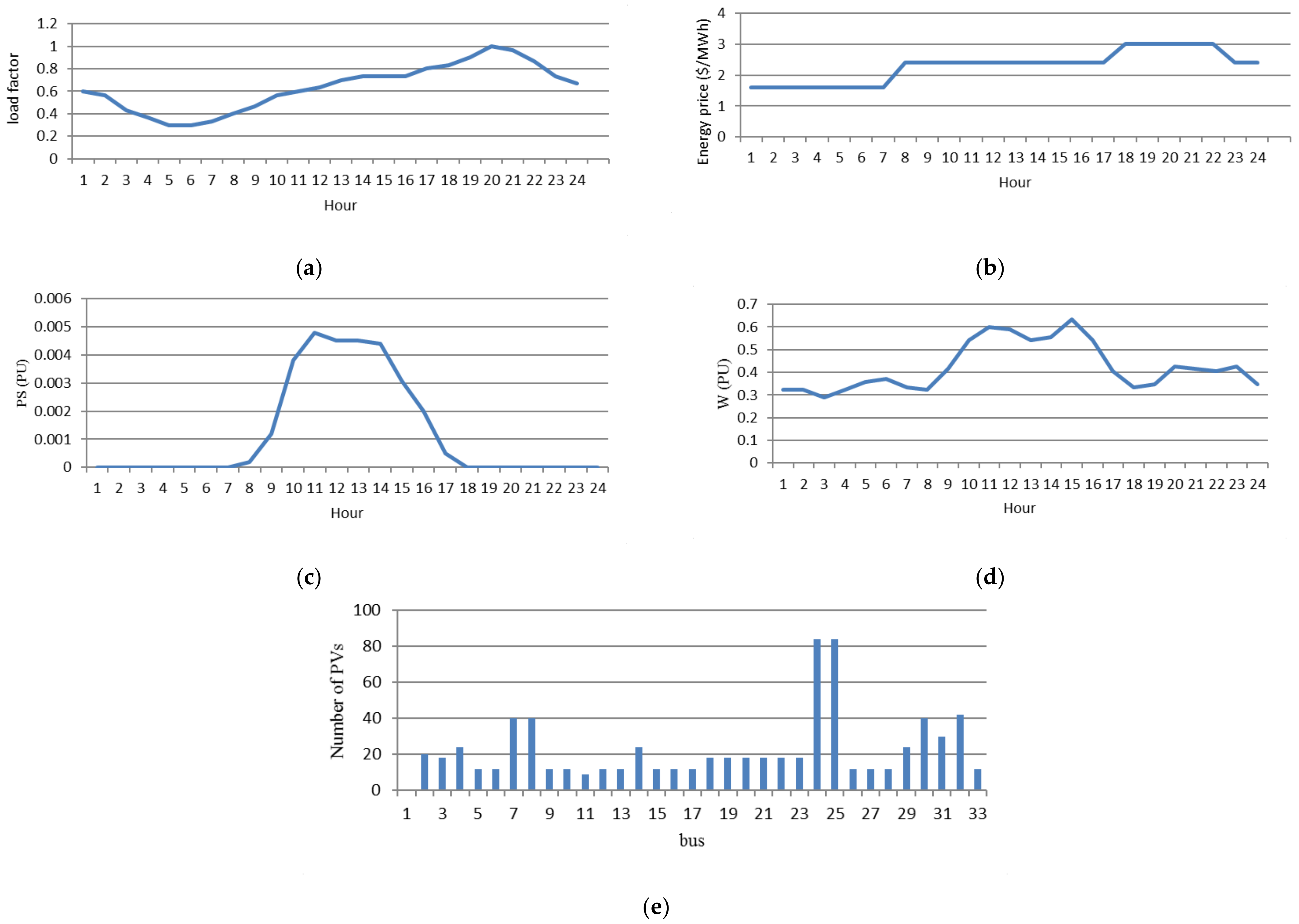
4.1. Data

The 33-bus distribution network is used to test the problem and is shown in [36]. The branch data for the 33-bus network is retrieved from [36]. It is worth mentioning that the base power and voltage are 1 MVA and 12.66 kV. The voltage magnitudes of buses are presumed to be within the range of 0.9 p.u. and 1.05 p.u. The peak demand of the system is fetched from [36]. The 33-bus distribution network’s required data are represented in Figure 2. Herein, we assume two wind units with the capacity of 800 kVA are located at buses 15 and 30. Herein, the PV units in each bus are controlled in an aggregated framework, and the capacity of each PV system is set at 5 kVA.

4.2. Results

The following three cases are studied:

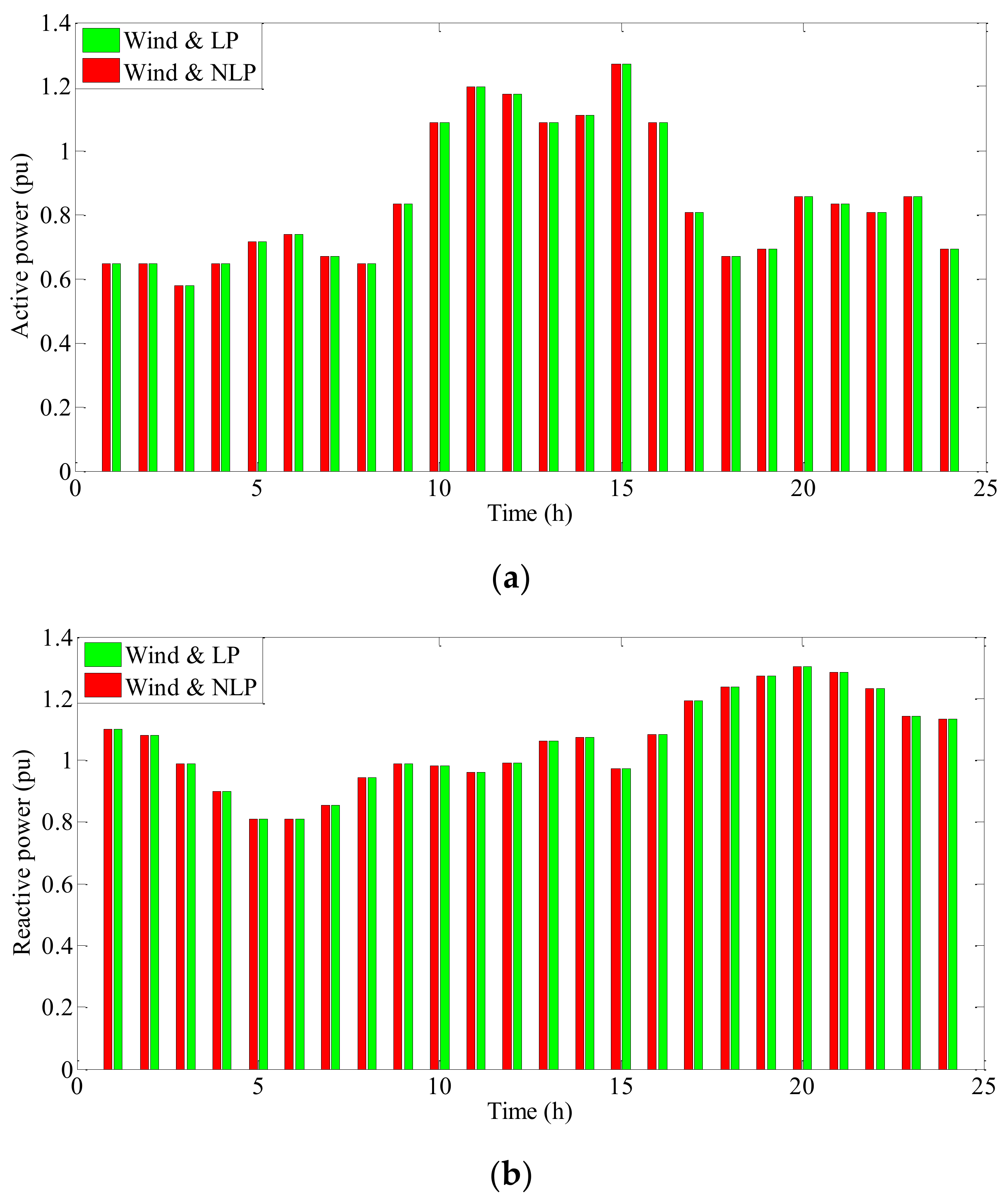
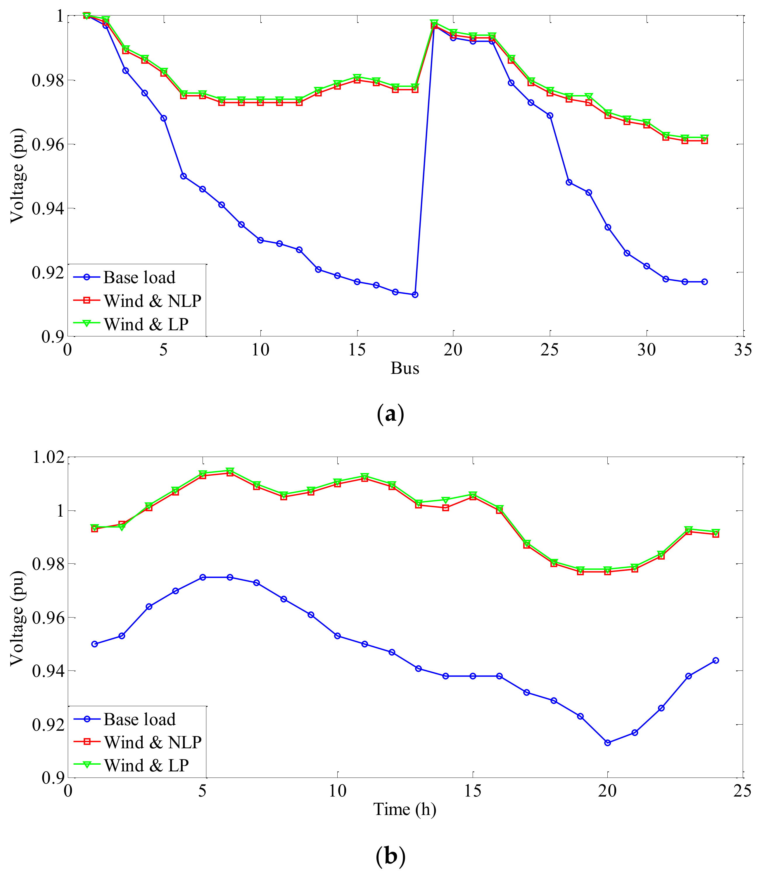
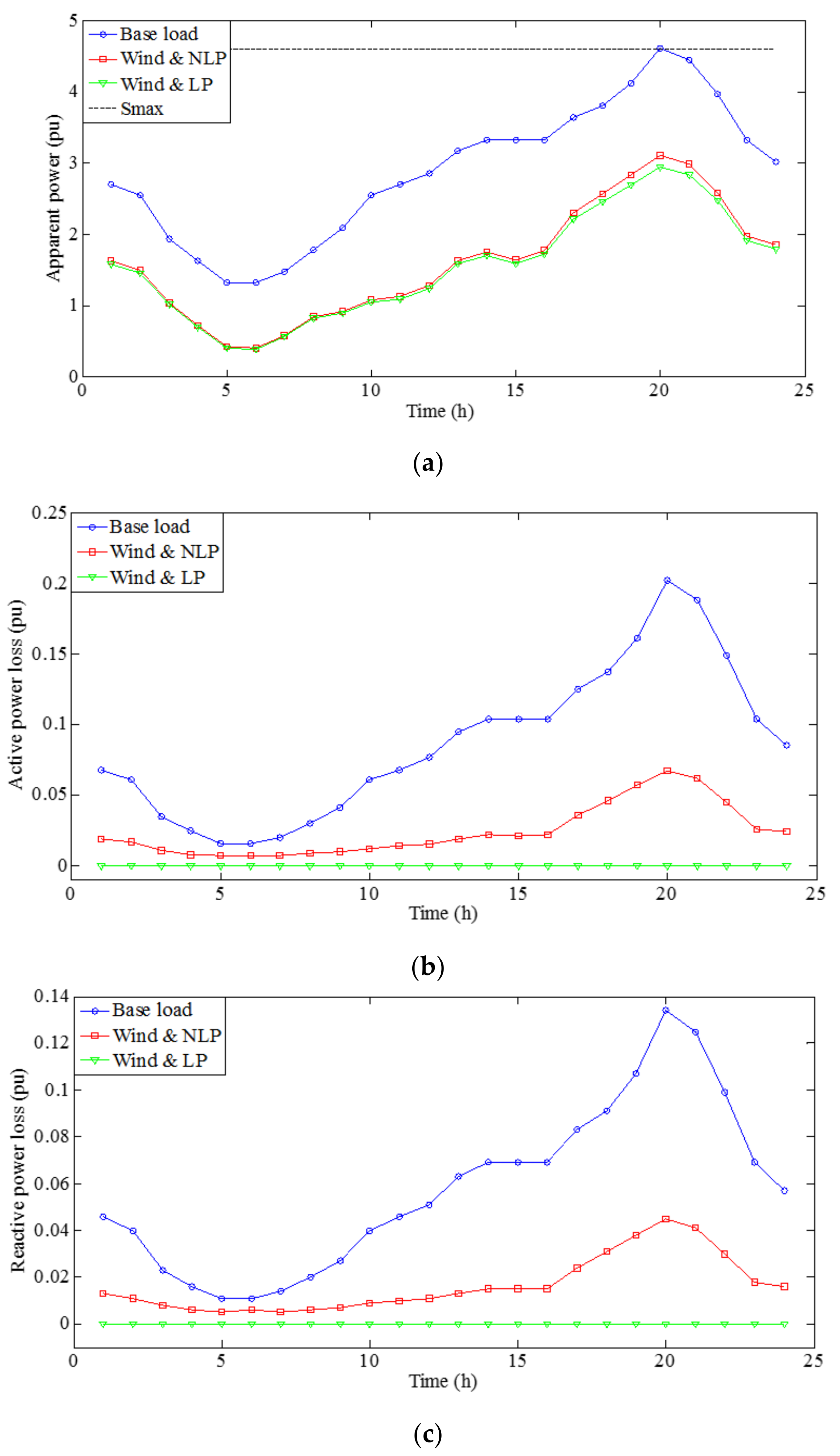
• Case A: power management of SDN in the presence of wind units.
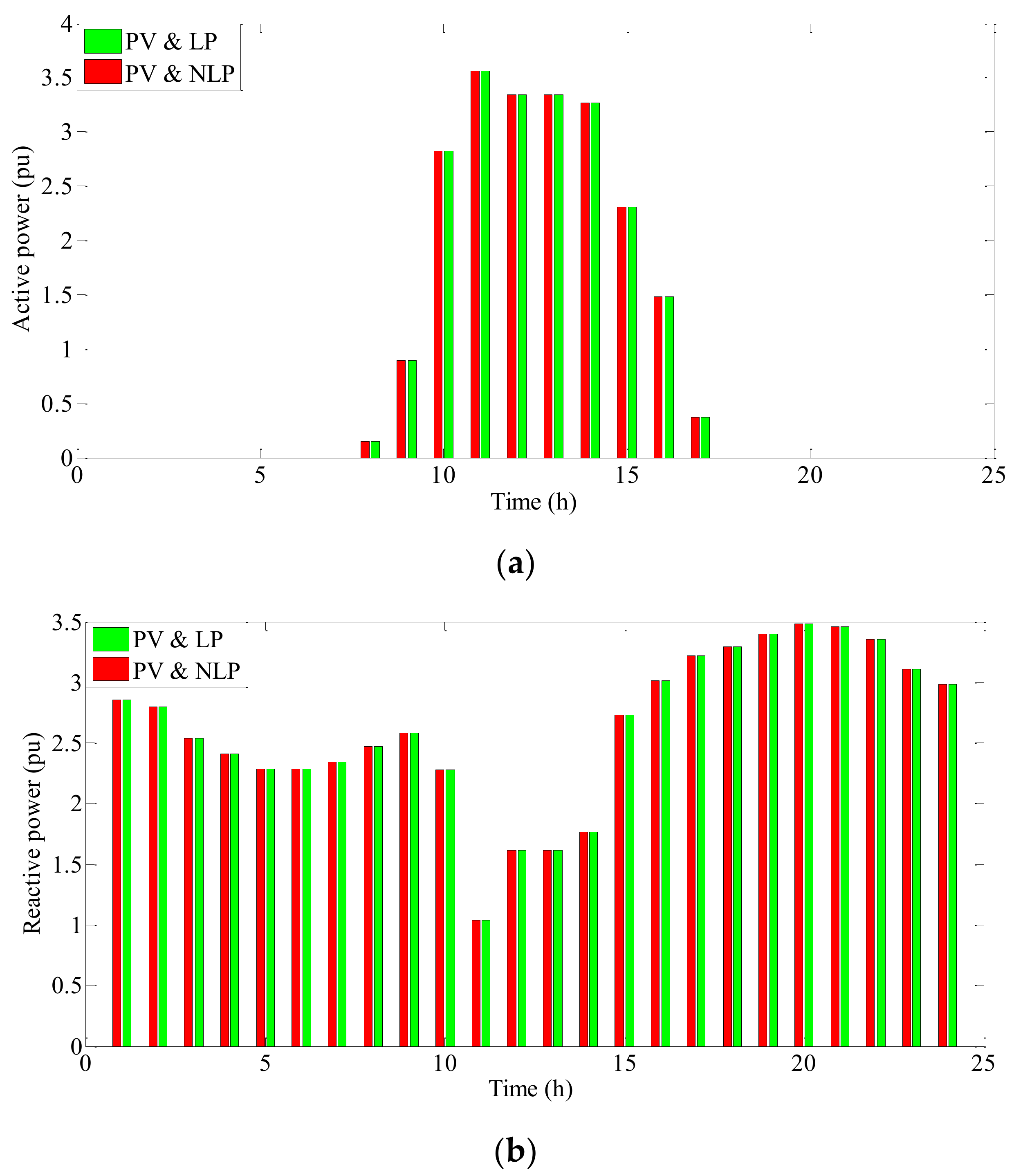
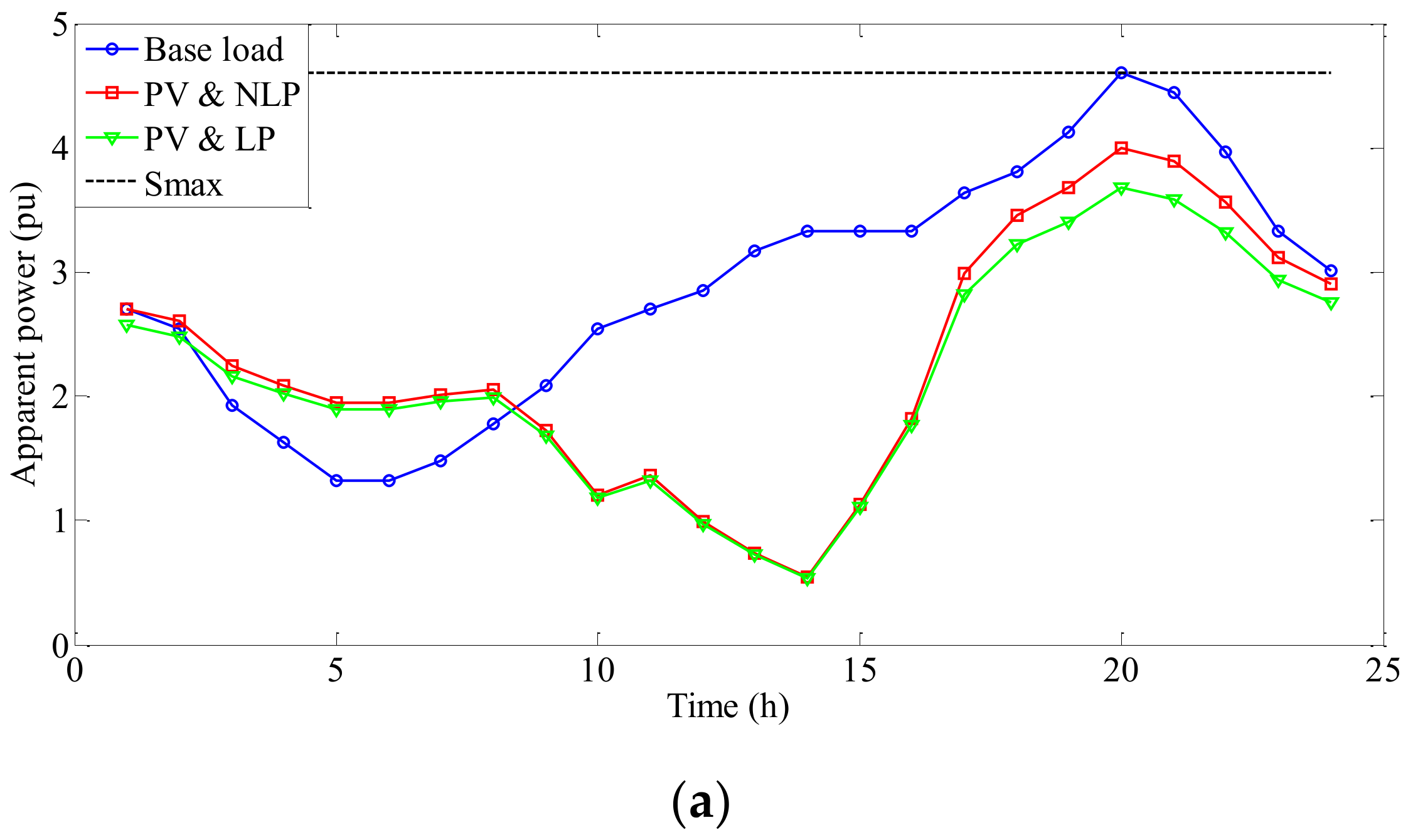
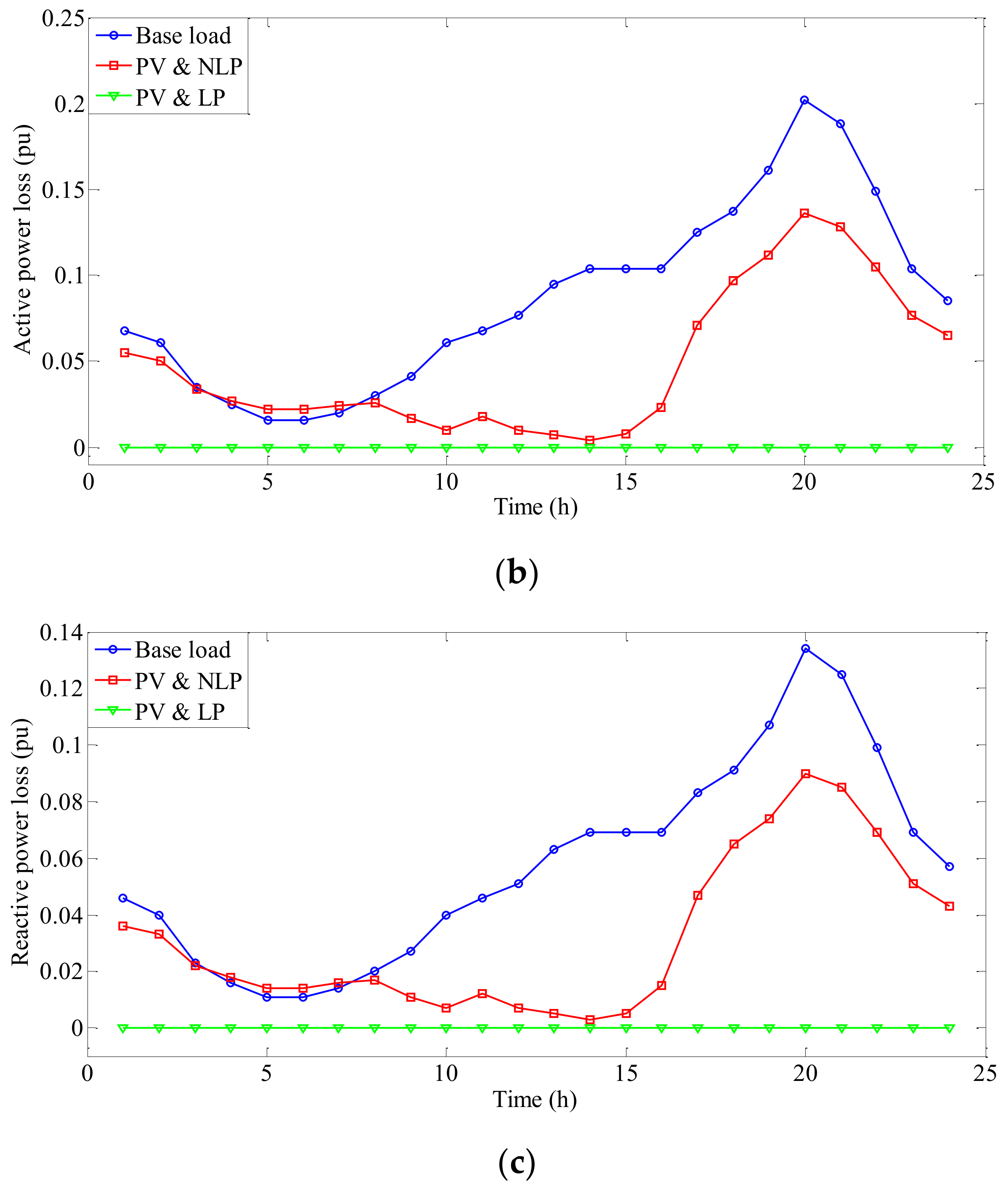
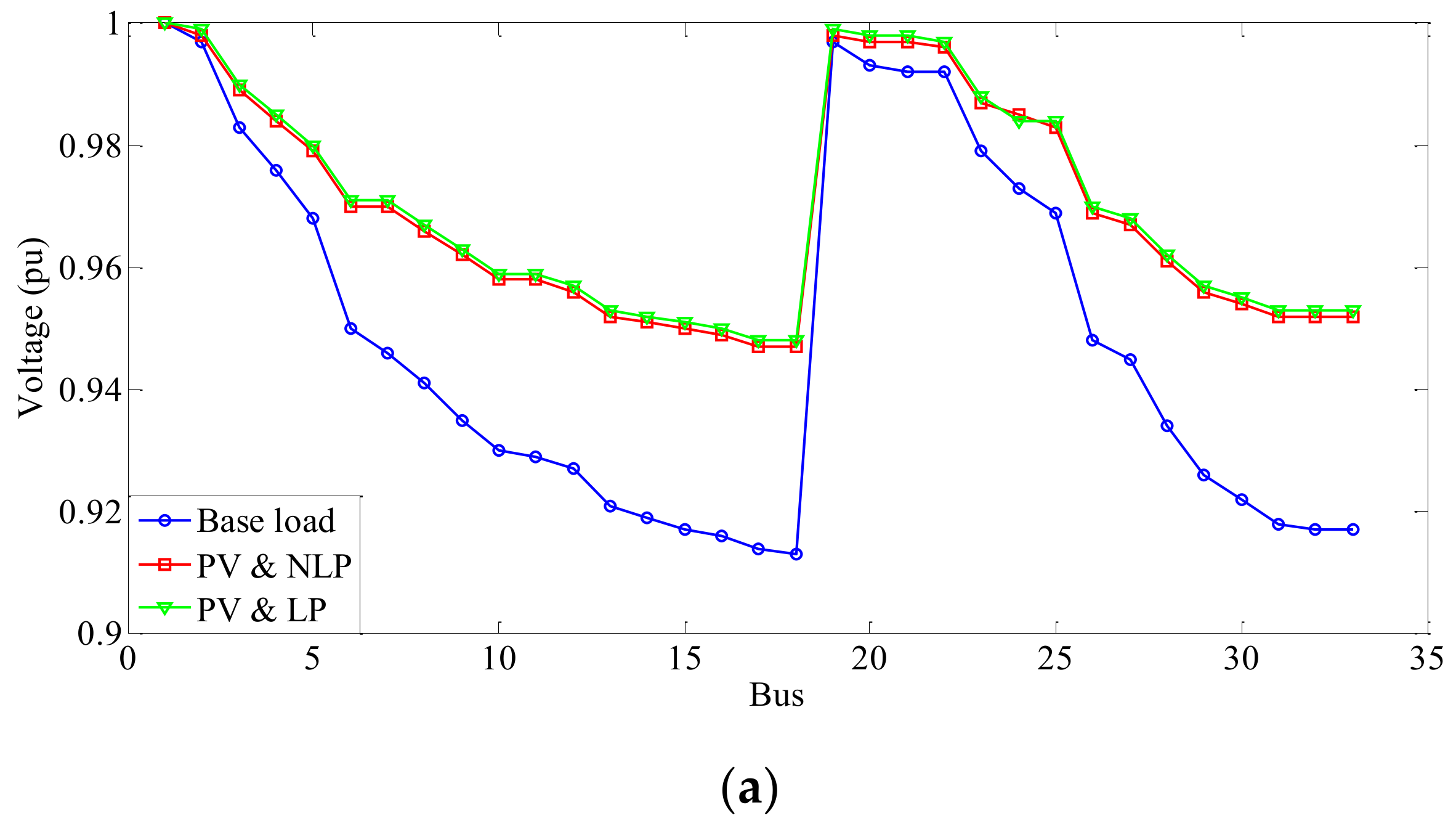
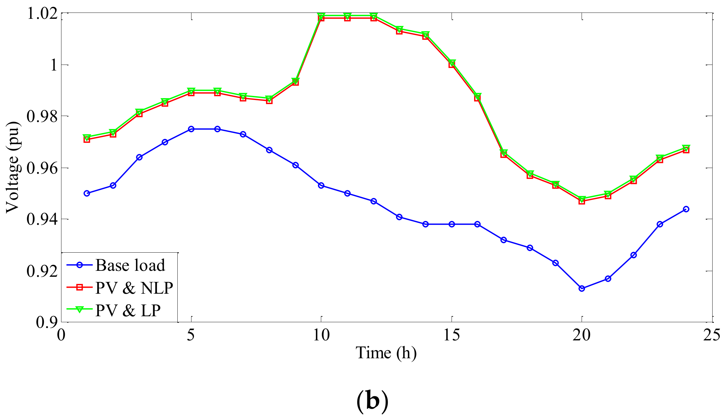
• Case B: power management of SDN in the presence of PV units.
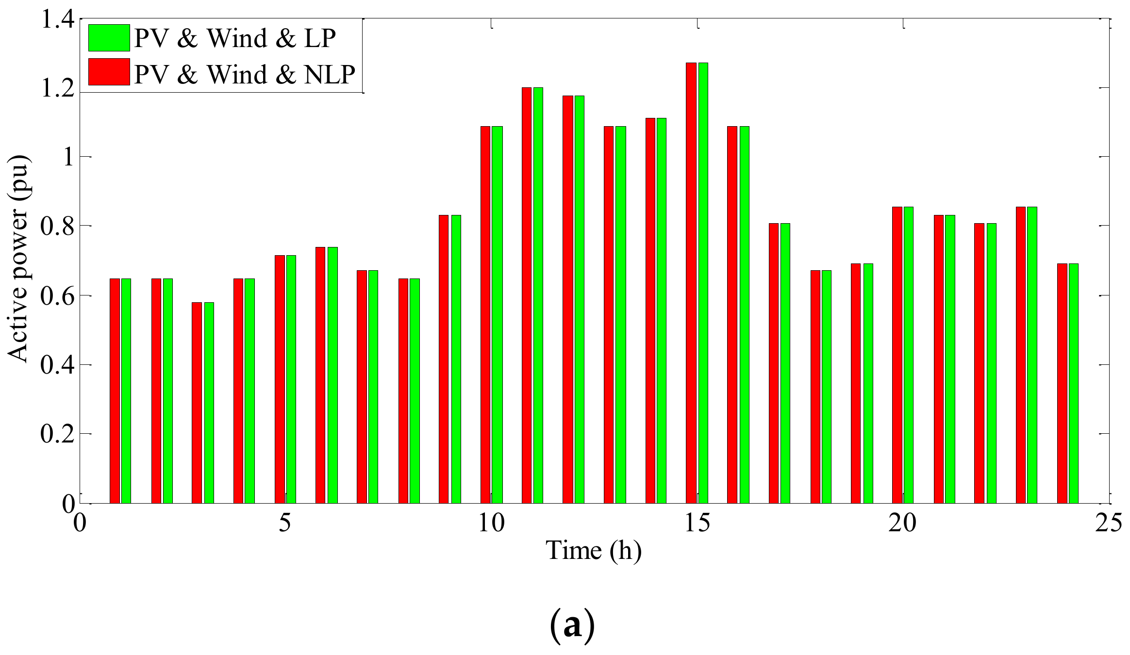
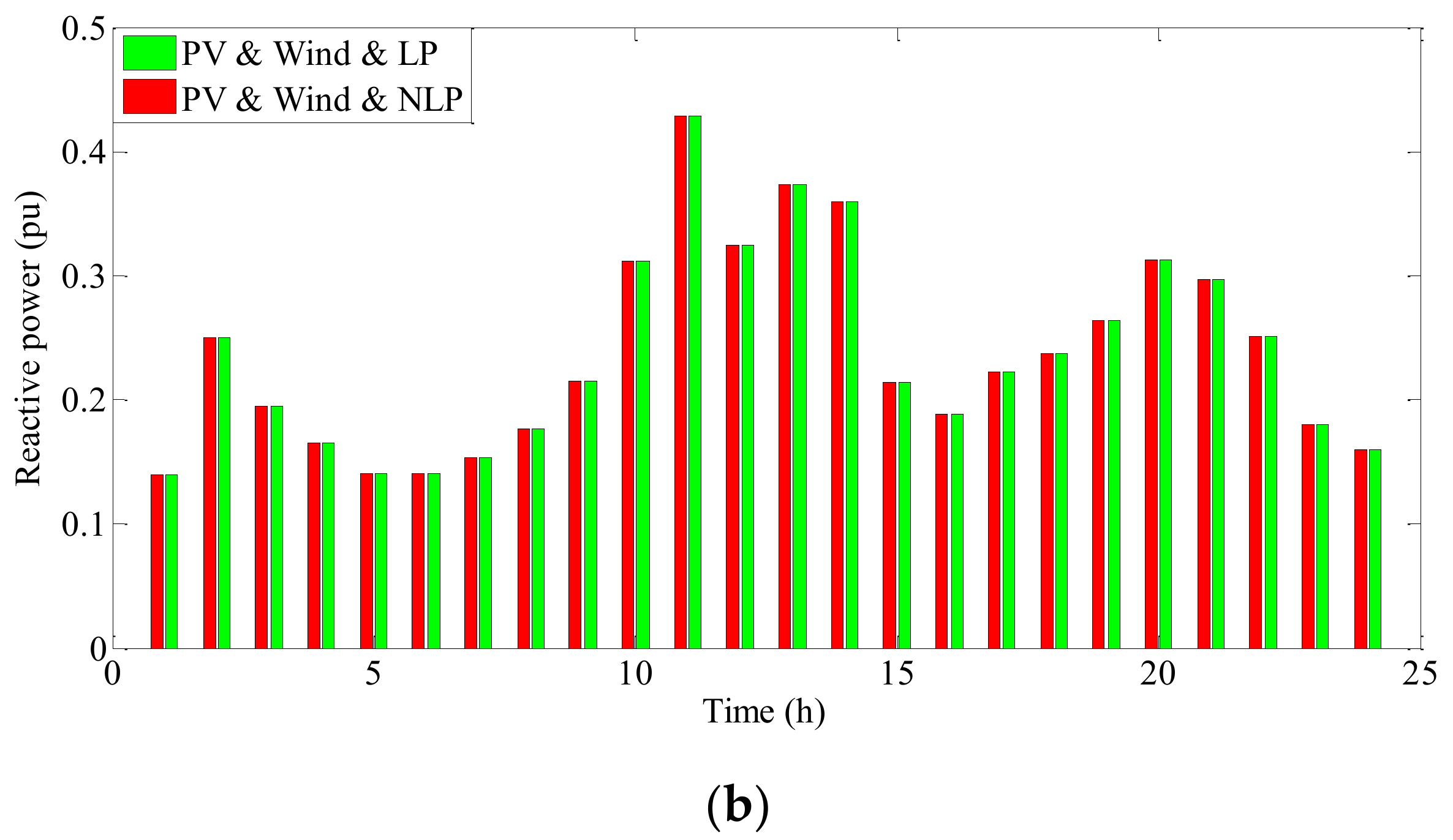
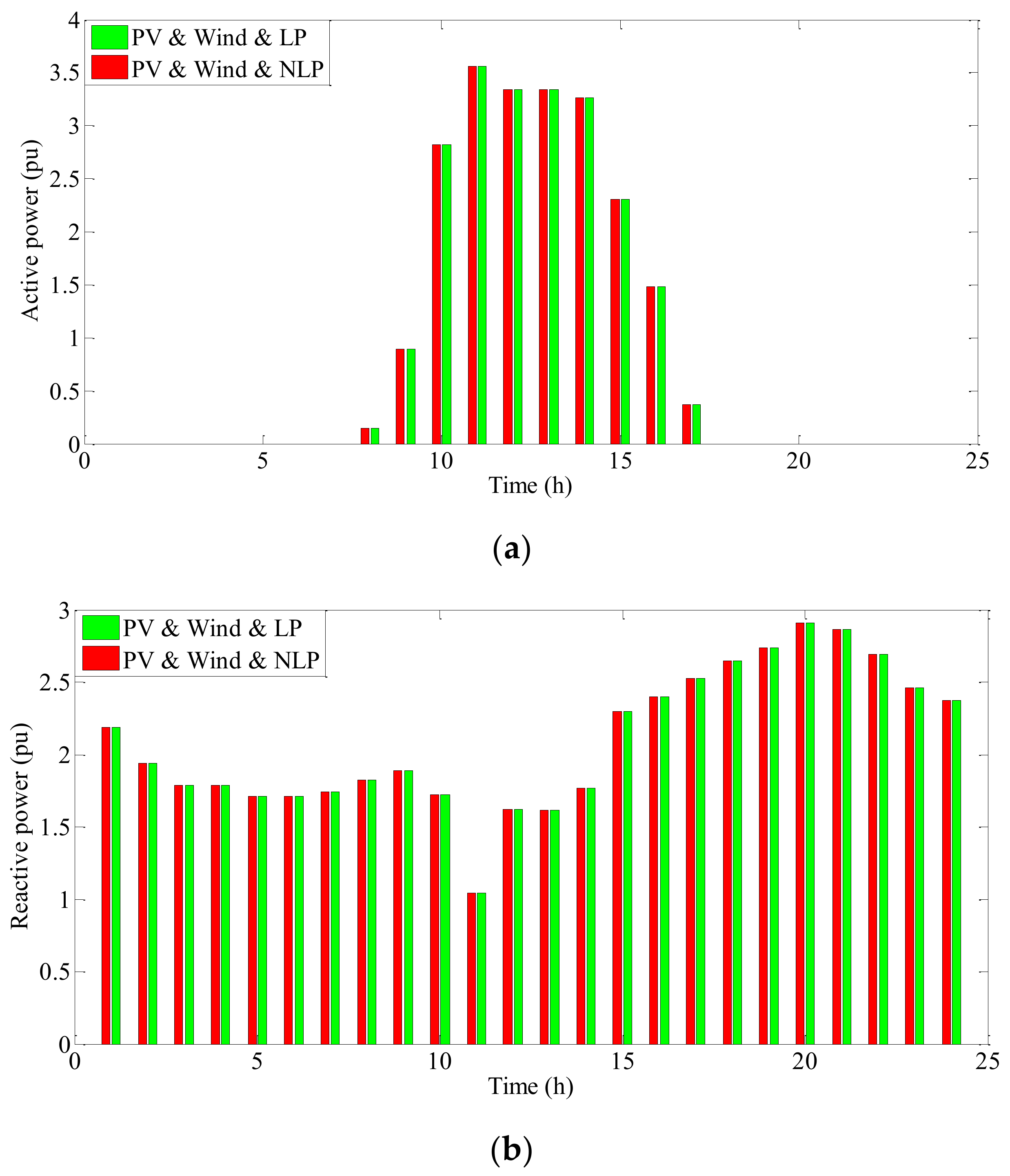
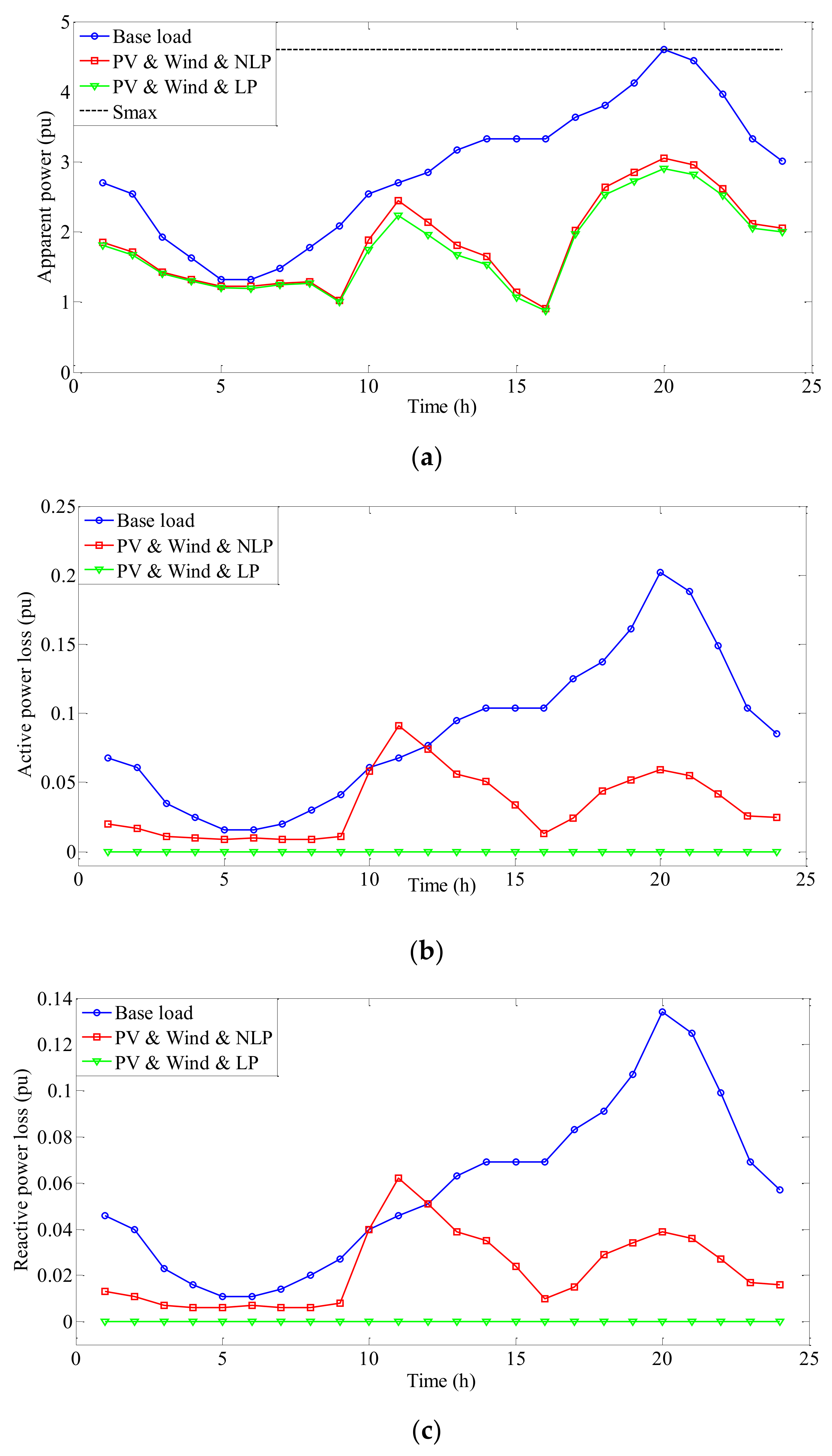
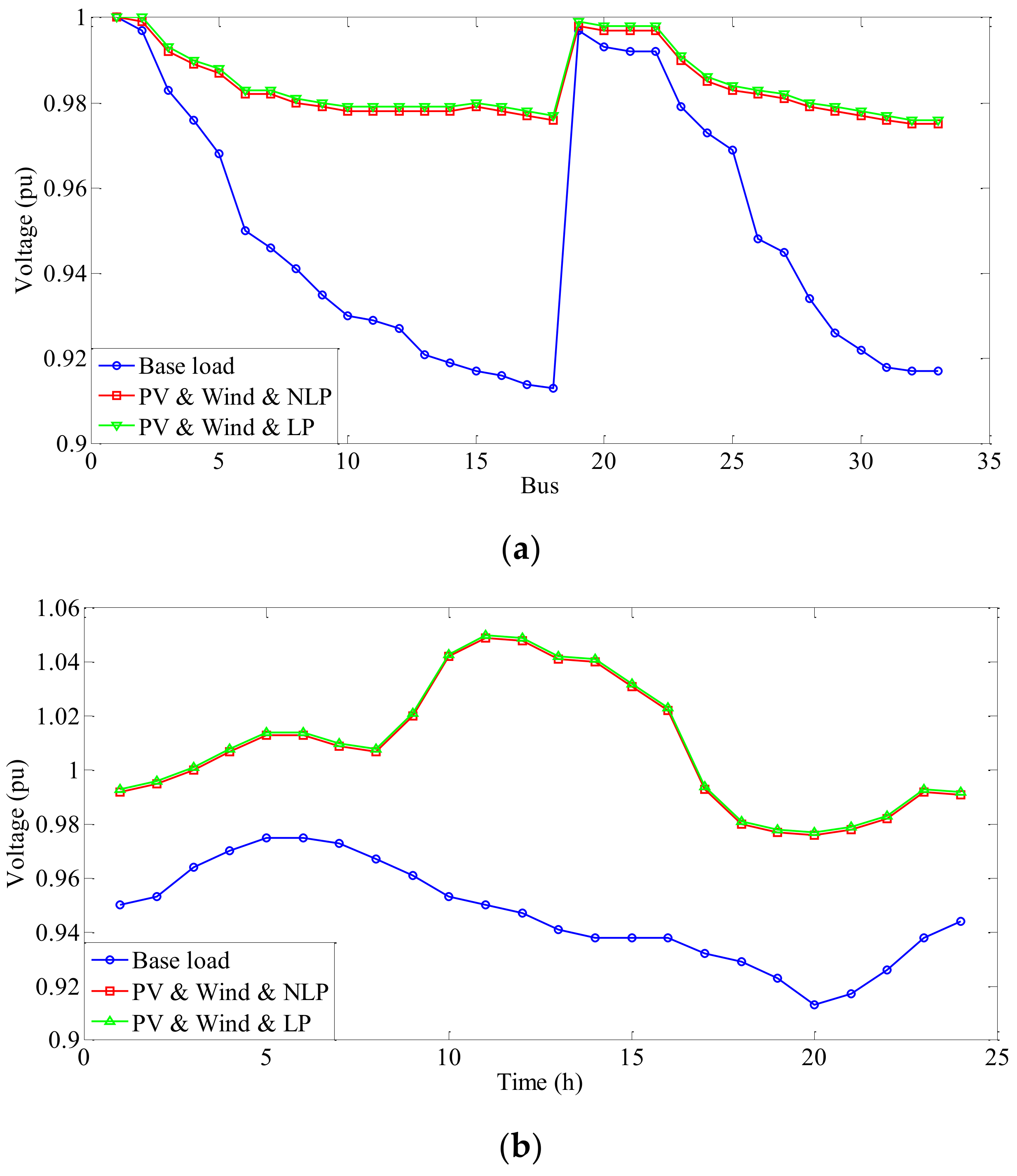
• Case C: power management of SDN penetrated with wind and PV units.

It is worth mentioning that the problem is solved for both the NLP and LP models for the cases above. The problem was solved by CONOPT/CPLEX solvers of the General Algebraic Modeling System (GAMS) software [37,38,39].

• Case A

In this case, active and reactive power management of SDNs penetrated with wind units is analyzed. Figure 3, Figure 4 and Figure 5 illustrate the results, including active and reactive power curves of wind units, apparent power curve, active and reactive network losses, voltage profile at peak period (20:00), and daily voltage curve of Bus 18. According to Figure 2a, the active power requirement of the grid is mainly provided by wind units due to its low operating costs. Additionally, according to Figure 3b, wind units have a high potential of constantly producing reactive power, which could remarkably reduce voltage deviations and network losses. As shown, the active and reactive power provided by wind units is similar in both NLP and LP models, which is stemmed from the unequal circular constraint for the wind unit approximated with a high number of planes (180 planes).

Figure 4 demonstrates the apparent daily power and active and reactive losses. As shown in Figure 4a, the graph of changes in apparent power is similar to the load profile shown in Figure 2a. Furthermore, the apparent power of the network in the presence of wind units is much lower than that of the case without wind unit’s penetration since a large volume of demand is met by the wind unit. Moreover, according to Figure 4b and Figure 6c, active and reactive power losses are reduced, which stem from local generations by wind units reducing the tension on congested transmission and distribution networks. In other words, the power loss of the system would be reduced. Additionally, note that in the LP model, due to the linearization of active and reactive power flow equations, the active and reactive losses of the network will be zero [40]. Since the network loss rate is about 3% of the total network load, it can be concluded that the computational error of the LP model would be about 3%. For instance, in Figure 4a, the apparent power at peak load time (20:00) for the NLP model is around 3 p.u. It is around 2.9 p.u. for the LP model. Therefore, the computational power error in the LP model compared to the NLP model is around 3% (3/(2.9–3)).

Figure 5 depicts the voltage profile of the network at the peak period (hour 20) and the daily voltage curve of Bus 18. According to Figure 5a, the highest voltage drop occurs without the presence of the wind unit. In contrast, the voltage drop rate is significantly reduced with the penetration of wind units. It is worth pointing out that the voltage magnitude of bus 18 is lower than other buses because Bus 18 has the longest distance from the reference bus than the rest of the buses. Hence, the line impedance and the loading are high. Additionally, the results advocate that the daily voltage magnitude would be improved with the penetration of wind units, as shown in Figure 5b. Furthermore, it can be seen that the maximum error for LP and NLP model in Figure 5 is minor. Thus, the LP model leads to a minute computational error for bus voltages.

• Case B

In this case, active and reactive power management of the SDN in the presence of PV systems is investigated. Figure 6 depicts the expected daily curve for active and reactive power of PVs. As can be seen, the PV unit provides a major share of the SDN active demands with low operational costs. Furthermore, considerable reactive power is fed into the main grid; so that the bus voltages approach one per unit. The PV inverter could also control the reactive power at night via switching. It can also be perceived that the results of both linear and nonlinear models are similar due to the precise approximation of the circular plane, which stems from using many sides.

Figure 7 and Figure 8 provide the apparent power, active and reactive power loss, and network voltage profile. As shown from Figure 7a, PVs’ active and reactive power production results in apparent power mitigation in the network during 9:00–00:00 h in both LP and NLP models, compared to case A. However, there is an increase in the apparent power of the network in this case due to the high injection of reactive power by PVs into the grid in comparison to case A. Similar trends for active and reactive losses are realized in this case. From Figure 8, it can be advocated that the PV consideration in the SDN flattens the voltage profile of the network. Last, the voltage difference of NLP and LP models is tangible in this case, with a maximum error of 0.5%.

• Case C

In this case, active and reactive power management of the SDN in the presence of both wind and PV systems is explored. Herein, nonlinear (Equations (1)–(15)) and linear (Equations (38) and Constraints) equations are regarded in the model. The daily active and reactive power curves generated by wind and PV units are presented in Figure 9 and Figure 10, respectively. As can be seen, a large share of the active demand is provided by renewable resources so as to minimize the system’s operating cost in case C. However, the reactive power is lower than in previous cases, resulting in lower power losses. The results pertained to the power losses, and the voltage profile of case C is shown in Figure 11 and Figure 12. As shown in Figure 11, the local renewable penetrations would reduce the apparent power received from the upstream network and reduce the active and reactive losses of the network compared to case A. Moreover, the voltage profile is smoother in this case compared to case A.

The results also advocate that the power losses in the LP model are zero as in previous cases, so the computational error for the active and reactive power of the network is around 3%. The calculation error of the voltage magnitude is about 0.5%.

• Comparison of case studies

In this section, the operating indicators such as active and reactive power losses during peak interval (hour 20), energy cost, and maximum voltage deviation for power flow studies of various case studies are tabulated in

Table 1. Value of Operation Indices in Different Case Studies.

Parameter	Power Loss (p.u.) at Hour 20:00				Energy Cost ($)		Maximum Voltage Deviation (p.u.)		Calculation Time (s)
	Active		Reactive
Model	LP	NLP	LP	NLP	LP	NLP	LP	NLP	LP		NLP
Uncertainty Model	UT								UT	SBSP	UT	SBSP
SDN without renewable penetration	0	0.221	0	0.130	3197	3225	0.0866	0.087	0.3	0.51	35	52
SDN with WS penetration (without reactive power control)	0	0.178	0	0.121	2438	2465	0.0546	0.054	1.28	1.61	125	159
SDN with WS penetration (with reactive power control)	0	0.135	0	0.96	2436	2463	0.0328	0.033	1.4	1.73	145	178
SDN with PV penetration (without reactive power control)	0	0.214	0	0.126	2835	2862	0.0723	0.072	1.5	1.88	155	190
SDN with PV penetration (with reactive power control)	0	0.206	0	0.102	2832	2859	0.0457	0.046	1.6	1.97	167	201
SDN with WS and PV penetration (without reactive power control)	0	0.172	0	0.119	2039	2066	0.0506	0.050	1.9	2.35	203	256
SDN with WS and PV (without reactive power control) and fixed capacitor bank penetration	0	0.163	0	0.112	2038	2065	0.0427	0.042	2.1	2.49	211	265
SDN with WS and PV (without reactive power control) and switched capacitor bank penetration	0	0.151	0	0.103	2037	2064	0.0356	0.035	2.9	3.43	254	302
SDN with WS and PV penetration (with reactive power control)	0	0.131	0	0.87	2037	2064	0.0218	0.022	2.1	2.54	219	272

. In case studies considering the presence of a fixed capacitor bank, it is usually assumed that they are located at buses 15, 18, 28, and 33 with a capacity of 0.3 MVAr, and the reactive power is always injected into the network. In this case, a term $+Q{C}_{i,o,\varpi }$ (Q_C, representing the reactive power of the capacitor bank) is placed to the left of Equation (3), and its value is equal to 0.3 in all simulation hours and scenarios in the mentioned buses. In the case studies using a switched capacitor bank, it is assumed that they are located on buses 15, 18, 28, and 33, and their capacity is 0.3 MVAr with five steps. As mentioned before, the term $+Q{C}_{i,o,\varpi }$ is added to the left of Equation (3). The constraint $Q{C}_{i,o,\varpi }=Q0\times x{C}_{i,o,\varpi }\hspace{0.17em}\hspace{0.17em}\hspace{0.17em}\hspace{0.17em}\forall i,o,\varpi ,xC\in \{1,2,3,4,5\}$ is also added to problem (38), where xC represents the integer variable corresponding to the operating step of the switched capacitive bank. Q0 is the reactive power per step, which is equal to 0.06 MVAr (0.3/5).

As is given in Table 1, the proposed LP model fails to calculate active and reactive power losses. However, the deviation of energy costs and maximum voltages in the LP model is intangible compared to the NLP model. More importantly, according to Table 1, the computational time is minute compared to the NLP model. Thus, the computational error can be neglected in return for the fast convergence of the LP model. Additionally, it can be seen that wind turbine penetration would reduce active power losses during peak hours. In contrast, when PV units are penetrated in the SDN, there is little effect on lowering active power losses in the system. Nonetheless, lower reactive power losses would be realized with PV units’ penetration. All things considered, the energy cost, reactive power, and computation time of the system reduce altogether remarkably with PV and WS penetrations.

The proposed design in the presence of wind and photovoltaic systems has been able to reduce active power losses by about 40.7% (0.221 (0.131–0.221)) compared to network load flow. Reactive power losses are reduced by about 33%, energy costs are reduced by 36%, and voltage deviations are reduced by about 74.7%. In addition, Table 1 presents the comparison results of computational time for the uncertainty modeling by UT and scenario-based stochastic programming (SBSP). In SBSP, a combination of Monte Carlo simulation (MCS) and Kantorovich simulation methods are used. MCS first generates a large number of scenarios (here 1000 scenarios). In each scenario, the number of uncertainties is determined based on their mean value and standard deviation, and then the probability of each selected amount of load and energy price is calculated from the normal probability distribution function. The probability of the power output of the wind system (photovoltaic system) is determined by the Weibull (Beta) probability distribution function. Afterward, the probability of each scenario is equal to the product of the probability of load, energy price, and renewable power. As a scenario reduction method, Kantorovich selects a certain number (here 50 scenarios) of the generated scenarios and applies them to the problem, so that their probability of occurrence is high and they are close to each other. Based on Table 1, it can be seen that the computational time of UT is less than the SBSP method.

It is noteworthy that according to Table 1, the RESs without reactive power control have less ability to improve operational indicators than the case with reactive power control. Of course, in this section, three cases are considered to control the reactive power, (1) the reactive power of the network is controlled by a fixed capacitor bank, (2) the reactive power of the network is controlled by a switched capacitor bank, (3) the reactive power of the network is controlled by the RESs. In case one, only a fixed value of reactive power is injected into the network; in case two, the change of reactive power injected into the network is stepwise, because the control of reactive power by the switched capacitor bank is reduced. In case three, however, the injectable reactive power changes continuously, as shown in Figure 9b and Figure 10b. According to Table 1, it can be seen that continuous control of reactive power has better results in improving the operational indicators such as power losses, voltage deviation, and energy cost.

5. Conclusions

The paper presented the problem of active and reactive power management of SDNs penetrated with wind units and aggregated PV systems. The units were equipped with power electronics converters to control the active and reactive powers. In the proposed model, the objective function aimed to minimize the expected operating cost of the system subjected to the AC power flow equations and the operating model of WSs and PVs. Moreover, the unscented transformation method was employed to model uncertainties associated with load, wind and PV power, and power prices. Then, a linear model was developed to burden the complexity of the nonlinear models. Lastly, the obtained numerical results indicated that the linear model had a lower computational error than the nonlinear model, around 3% and 0.5%, respectively, for active and reactive power of the network and voltage magnitude. Since the linear model’s convergence was faster than that of the nonlinear model, the obtained linear model was an appropriate approximation for the nonlinear model in the proposed model. The computational time was reduced to around 2 to 3 s, while the accurate model was around 200 to 250 s. Moreover, renewables penetration not only provided low-cost power to consumers but also improved the voltage of the system. On the whole, the proposed scheme simultaneously decreased active and reactive power losses, energy costs, and voltage deviations, so that these indices were reduced (improved) by around 40.7%, 33%, 36%, and 74.7%, respectively, in the proposed scheme compared to network load flow studies.

References

1. Ganesan, S.; Subramaniam, U.; Ghodke, A.A.; Elavarasan, R.M.; Raju, K.; Bhaskar, M.S. Investigation on Sizing of Voltage Source for a Battery Energy Storage System in Microgrid with Renewable Energy Sources. IEEE Access 2020, 8, 188861–188874. [Google Scholar] [CrossRef]
2. Azimian, M.; Amir, V.; Javadi, S. Economic and Environmental Policy Analysis for Emission-Neutral Multi-Carrier Microgrid Deployment. Appl. Energy 2020, 277, 115609. [Google Scholar] [CrossRef]
3. Fan, S.; Wang, Y.; Cao, S.; Zhao, B.; Sun, T.; Liu, P. A deep residual neural network identification method for uneven dust accumulation on photovoltaic (PV) panels. Energy 2021, 239, 122302. [Google Scholar] [CrossRef]
4. Han, J.; Choi, C.-S.; Park, W.-K.; Lee, I.; Kim, S.-H. Smart home energy management system including renewable energy based on ZigBee and PLC. IEEE Trans. Consum. Electron. 2014, 60, 198–202. [Google Scholar] [CrossRef]
5. Amir, V.; Azimian, M. Dynamic Multi-Carrier Microgrid Deployment Under Uncertainty. Appl. Energy 2020, 260, 114293. [Google Scholar] [CrossRef]
6. Norouzi, M.; Aghaei, J.; Pirouzi, S.; Niknam, T.; Fotuhi-Firuzabad, M.; Shafie-Khah, M. Hybrid stochastic/robust flexible and reliable scheduling of secure networked microgrids with electric springs and electric vehicles. Appl. Energy 2021, 300, 117395. [Google Scholar] [CrossRef]
7. Lekvan, A.A.; Habibifar, R.; Moradi, M.; Khoshjahan, M.; Nojavan, S.; Jermsittiparsert, K. Robust optimization of renewable-based multi-energy micro-grid integrated with flexible energy conversion and storage devices. Sustain. Cities Soc. 2021, 64, 102532. [Google Scholar] [CrossRef]
8. Pirouzi, S.; Aghaei, J.; Niknam, T.; Khooban, M.H.; Dragicevic, T.; Farahmand, H.; Korpas, M.; Blaabjerg, F. Power Conditioning of Distribution Networks via Single-Phase Electric Vehicles Equipped. IEEE Syst. J. 2019, 13, 3433–3442. [Google Scholar] [CrossRef] [Green Version]
9. Dini, A.; Pirouzi, S.; Norouzi, M.; Lehtonen, M. Hybrid stochastic/robust scheduling of the grid-connected microgrid based on the linear coordinated power management strategy. Sustain. Energy Grids Netw. 2020, 24, 100400. [Google Scholar] [CrossRef]
10. Habibifar, R.; Saber, H.; Gharigh, M.R.K.; Ehsan, M. Planning Framework for BESSs in Microgrids (MGs) Using Linearized AC Power Flow Approach. In Proceedings of the 2018 Smart Grid Conference (SGC), Sanandaj, Iran, 28–29 November 2018. [Google Scholar]
11. Saber, H.; Mazaheri, H.; Ranjbar, H.; Moeini-Aghtaie, M.; Lehtonen, M. Utilization of in-pipe hydropower renewable energy technology and energy storage systems in mountainous distribution networks. Renew. Energy 2021, 172, 789–801. [Google Scholar] [CrossRef]
12. Malekpour, A.R.; Pahwa, A. Reactive power and voltage control in distribution systems with photovoltaic generation. In Proceedings of the 2012 North American Power Symposium (NAPS), Champaign, IL, USA, 9–11 September 2012. [Google Scholar]
13. Turitsyn, K.; Sulc, P.; Backhaus, S.; Chertkov, M. Local control of reactive power by distributed photovoltaic generators. In Proceedings of the 2010 First IEEE International Conference on Smart Grid Communications, Gaithersburg, MD, USA, 4–6 October 2010. [Google Scholar]
14. Kobayashi, H.; Hatta, H. Reactive power control method between DG using ICT for proper voltage control of utility distribution system. In Proceedings of the 2011 IEEE Power and Energy Society General Meeting, Detroit, MI, USA, 24–28 July 2011. [Google Scholar]
15. Prenc, R.; Škrlec, D.; Komen, V. Optimal PV system placement in a distribution network on the basis of daily power consumption and production fluctuation. In Proceedings of the Eurocon 2013, Zagreb, Croatia, 1–4 July 2013; pp. 777–783. [Google Scholar] [CrossRef]
16. Azarhooshang, A.; Sedighizadeh, D.; Sedighizadeh, M. Two-stage stochastic operation considering day-ahead and real-time scheduling of microgrids with high renewable energy sources and electric vehicles based on multi-layer energy management system. Electr. Power Syst. Res. 2021, 201, 107527. [Google Scholar] [CrossRef]
17. Kiani, H.; Hesami, K.; Azarhooshang, A.; Pirouzi, S.; Safaee, S. Adaptive robust operation of the active distribution network including renewable and flexible sources. Sustain. Energy Grids Netw. 2021, 26, 100476. [Google Scholar] [CrossRef]
18. Yang, Z.; Ghadamyari, M.; Khorramdel, H.; Alizadeh, S.M.S.; Pirouzi, S.; Milani, M.; Banihashemi, F.; Ghadimi, N. Robust multi-objective optimal design of islanded hybrid system with renewable and diesel sources/stationary and mobile energy storage systems. Renew. Sustain. Energy Rev. 2021, 148, 111295. [Google Scholar] [CrossRef]
19. Asl, S.A.F.; Bagherzadeh, L.; Pirouzi, S.; Norouzi, M.; Lehtonen, M. A new two-layer model for energy management in the smart distribution network containing flexi-renewable virtual power plant. Electr. Power Syst. Res. 2021, 194, 107085. [Google Scholar] [CrossRef]
20. Dini, A.; Hassankashi, A.; Pirouzi, S.; Lehtonen, M.; Arandian, B.; Baziar, A.A. A flexible-reliable operation optimization model of the networked energy hubs with distributed generations, energy storage systems and demand response. Energy 2022, 239, 121923. [Google Scholar] [CrossRef]
21. Afrashi, K.; Bahmani-Firouzi, B.; Nafar, M. IGDT-Based Robust Optimization for Multicarrier Energy System Management. Iran. J. Sci. Technol. Trans. Electr. Eng. 2021, 45, 155–169. [Google Scholar] [CrossRef]
22. Homayoun, R.; Bahmani-Firouzi, B.; Niknam, T. Multi-objective operation of distributed generations and thermal blocks in microgrids based on energy management system. IET Gener. Transm. Distrib. 2021, 15, 1451–1462. [Google Scholar] [CrossRef]
23. Shahbazi, A.; Aghaei, J.; Pirouzi, S.; Niknam, T.; Shafie-Khah, M.; Catalão, J.P. Effects of resilience-oriented design on distribution networks operation planning. Electr. Power Syst. Res. 2020, 191, 106902. [Google Scholar] [CrossRef]
24. Norouzi, M.; Aghaei, J.; Pirouzi, S.; Niknam, T.; Lehtonen, M. Flexible operation of grid-connected microgrid using ES. IET Gener. Transm. Distrib. 2020, 14, 254–264. [Google Scholar] [CrossRef]
25. Pirouzi, S.; Aghaei, J.; Shafie-Khah, M.; Osorio, G.J.; Catalao, J.P.S. Evaluating the Security of Electrical Energy Distribution Networks in the Presence of Electric Vehicles. In Proceedings of the 2017 IEEE Manchester PowerTech, Manchester, UK, 18–22 June 2017. [Google Scholar]
26. Baziar, A.; Bo, R.; Ghotbabadi, M.D.; Veisi, M.; Rehman, W.U. Evolutionary Algorithm-Based Adaptive Robust Optimization for AC Security Constrained Unit Commitment Considering Renewable Energy Sources and Shunt FACTS Devices. IEEE Access 2021, 9, 123575–123587. [Google Scholar] [CrossRef]
27. Guo, C.; Ye, C.; Ding, Y.; Wang, P. A Multi-State Model for Transmission System Resilience Enhancement Against Short-Circuit Faults Caused by Extreme Weather Events. IEEE Trans. Power Deliv. 2020, 36, 2374–2385. [Google Scholar] [CrossRef]
28. Zhu, D.; Wang, B.; Ma, H.; Wang, H. Evaluating the vulnerability of integrated electricity-heat-gas systems based on the high-dimensional random matrix theory. CSEE J. Power Energy Syst. 2020, 6, 878–889. [Google Scholar]
29. Roustaee, M.; Kazemi, A. Multi-objective energy management strategy of unbalanced multi-microgrids considering technical and economic situations. Sustain. Energy Technol. Assess. 2021, 47, 101448. [Google Scholar] [CrossRef]
30. Pirouzi, S.; Aghaei, J. Mathematical modeling of electric vehicles contributions in voltage security of smart distribution networks. Simulation 2018, 95, 429–439. [Google Scholar] [CrossRef]
31. Dabbaghjamanesh, M.; Kavousi-Fard, A.; Mehraeen, S. Effective Scheduling of Reconfigurable Microgrids with Dynamic Thermal Line Rating. IEEE Trans. Ind. Electron. 2018, 66, 1552–1564. [Google Scholar] [CrossRef]
32. Papari, B.; Edrington, C.S.; Ghadamyari, M.; Ansari, M.; Ozkan, G.; Chowdhury, B.H. Metrics Analysis Framework of Control and Management System for Resilient Connected Community Microgrids. IEEE Trans. Sustain. Energy 2022, 13, 704–714. [Google Scholar] [CrossRef]
33. Zhang, L.; Gao, T.; Cai, G.; Hai, K.L. Research on electric vehicle charging safety warning model based on back propagation neural network optimized by improved gray wolf algorithm. J. Energy Storage 2022, 49, 104092. [Google Scholar] [CrossRef]
34. Zafarani, H.; Taher, S.A.; Shahidehpour, M. Robust operation of a multicarrier energy system considering EVs and CHP units. Energy 2020, 192, 116703. [Google Scholar] [CrossRef]
35. Habibifar, R.; Ranjbar, H.; Shafie-Khah, M.; Ehsan, M.; Catalao, J.P.S. Network-Constrained Optimal Scheduling of Multi-Carrier Residential Energy Systems: A Chance-Constrained Approach. IEEE Access 2021, 9, 86369–86381. [Google Scholar] [CrossRef]
36. Babu, P.R.; Rakesh, C.P.; Kumar, M.N.; Srikanth, G.; Reddy, D.P. A Novel Approach for Solving Distribution Networks. In Proceedings of the 2009 Annual IEEE India Conference, Ahmedabad, India, 18–20 December 2009. [Google Scholar]
37. General Algebraic Modeling System (GAMS). Available online: https://www.gams.com/ (accessed on 20 September 2021).
38. Shahbazi, A.; Aghaei, J.; Pirouzi, S.; Shafie-Khah, M.; Catalão, J.P. Hybrid stochastic/robust optimization model for resilient architecture of distribution networks against extreme weather conditions. Int. J. Electr. Power Energy Syst. 2021, 126, 106576. [Google Scholar] [CrossRef]
39. Aghaei, J.; Bozorgavari, S.A.; Pirouzi, S.; Farahmand, H.; Korpås, M. Flexibility Planning of Distributed Battery Energy Storage Systems in Smart Distribution Networks. Iran. J. Sci. Technol. Trans. Electr. Eng. 2020, 44, 1105–1121. [Google Scholar] [CrossRef]
40. Ansari, M.; Pirouzi, S.; Kazemi, M.; Naderipour, A.; Benbouzid, M. Renewable Generation and Transmission Expansion Planning Coordination with Energy Storage System: A Flexibility Point of View. Appl. Sci. 2021, 11, 3303. [Google Scholar] [CrossRef]
Figure 1. Linearization method of the circular plane.
Sustainability 14 04273 g001
Figure 2. System’s data; (a) load factor [9], (b) energy price [9], (c) PV active power [19], (d) wind system active power [19], (e) PVs number in each bus.
Sustainability 14 04273 g002
Figure 3. Expected daily curve: (a) active power, (b) reactive power in case A.
Sustainability 14 04273 g003
Figure 4. Expected daily curve: (a) apparent power, (b) active power loss, (c) reactive power loss in case A.
Sustainability 14 04273 g004
Figure 5. (a) expected voltage profile of buses at hour 20, (b) expected daily voltage curve of Bus 18 in case A.
Sustainability 14 04273 g005
Figure 6. Expected daily curve of, (a) active power, (b) reactive power in Case B.
Sustainability 14 04273 g006
Figure 7. Expected daily curve of, (a) apparent power, (b) active power loss, (c) reactive power loss in case B.
Sustainability 14 04273 g007aSustainability 14 04273 g007b
Figure 8. (a) Expected voltage profile at hour 20, (b) expected daily voltage curve of Bus 18 in case B.
Sustainability 14 04273 g008aSustainability 14 04273 g008b
Figure 9. Expected daily curve of, (a) active power, (b) reactive power for all wind systems in case C.
Sustainability 14 04273 g009aSustainability 14 04273 g009b
Figure 10. Expected daily curve of, (a) active power, (b) reactive power for all PVs in case C.
Sustainability 14 04273 g010
Figure 11. Expected daily curve of, (a) apparent power, (b) active power loss, (c) reactive power loss in case C.
Sustainability 14 04273 g011
Figure 12. (a) Expected voltage profile at hour 20, (b) expected daily voltage curve of Bus 18 in case C.
Sustainability 14 04273 g012