1. Introduction
Public transport companies are confronted with major challenges. As a climate-friendly alternative to the private car, great hopes are pinned on public transport to tackle the climate crisis by providing a more sustainable means of transport. Germany, for example, wants to double the number of public transport passengers by 2030 compared to 2010, according to its climate action plans. Achieving this goal will only be possible through large investments, an increased attractiveness and optimized planning. While investments in public transport are the responsibility of the government at the federal and regional levels, increased attractiveness and optimized planning are goals that can also be supported by research and the development of new technologies. Specifically optimized planning requires accurate information about the demand, operation, and optimization possibilities of public passenger transport. The planning and operation of public transport already involves a multitude of data sources. The ongoing digitization of public transport makes new data sources accessible and has greatly increased the amount of data available in recent years and decades already. These data sources, in turn, generate a high volume of data in a wide variety of formats and data rates. However, many challenges in public transport planning at the moment stem from a lack of coherent information and transport companies are currently not able to exploit the full potential of their data. The application of data science methods to the vast amount of data in public transport could be the key needed to fill the information gap and to provide a foundation for the further expansion of public transport. In this paper, we present our systematic approach to recognize and tap into this potential. We present our approaches to utilize public transport data and discuss the lessons we learned. We hope to demonstrate that the public transport domain offers numerous valuable use cases for data scientists to explore as well as to clarify the potential of data science methods for representatives of the public transport domain. We identify challenges for the application of data science on public transport data and propose solutions to highlight a path towards data management in public transport that enables the efficient and successful application of data science methods. We are firmly convinced that these developments can improve public transport and greatly contribute to develop public transport into an even more important pillar of sustainable mobility in the future.
First, we identify and categorize the data sources generally available to transport companies and review several approaches towards data collection and data analysis for public transport.
Section 2 describes these categories and data sources, as well as related work for data science methods in these data source categories. Based on this classification, we then provide an overview of the use cases that transport companies can fulfil by analyzing these data. We interview representatives of public transport associations as well as representatives from several companies developing software for public transport about the use cases for which they envision utilizing their data and about their current problems that stem from a lack of coherent information. In
Section 3, we discuss the use cases we identified as well as recent approaches to these use cases from the literature. The resulting classification can structure the discussion of how and where to apply data science methods in public transport, specifically discussions in the public transport domain itself. In our current and ongoing work, we use data science methods to explore the application of public transport data to some of the use cases. We report on the use cases that we explored and describe our findings in
Section 4. In
Section 5, we describe the difficulties we encountered and discuss how the characteristics of public transport and data sources in public transport entail challenges for data science and the application of machine learning methods. Based on these challenges, we discuss open research questions and future work as well as organizational challenges for public transport companies as solution approaches.
Section 6 concludes this paper with a summary and outlook. The solution approaches discussed lay out a path for the improvement of public transport.
2. Categorization of Data Sources in Public Transport
To understand data sources in public transport and to identify which data sources are currently einvestigated and used, we interviewed representatives of public transport agencies and reviewed three meta-studies investigating those data sources. In their meta-study, Maria Karatsoli and Eftihia Nathanail looked at 69 studies from the field of transport research [
1]. Of these studies, 14 deal with public transport issues. Khatun E. Zannat and Charisma F. Choudhury limited their analysis to studies that used big data in the field of public transport planning [
2]. They examined a total of 47 publications.
Timothy F. Welch and Alyas Widita evaluated 81 publications [
3]. They focused on data sources in the field of public transport.
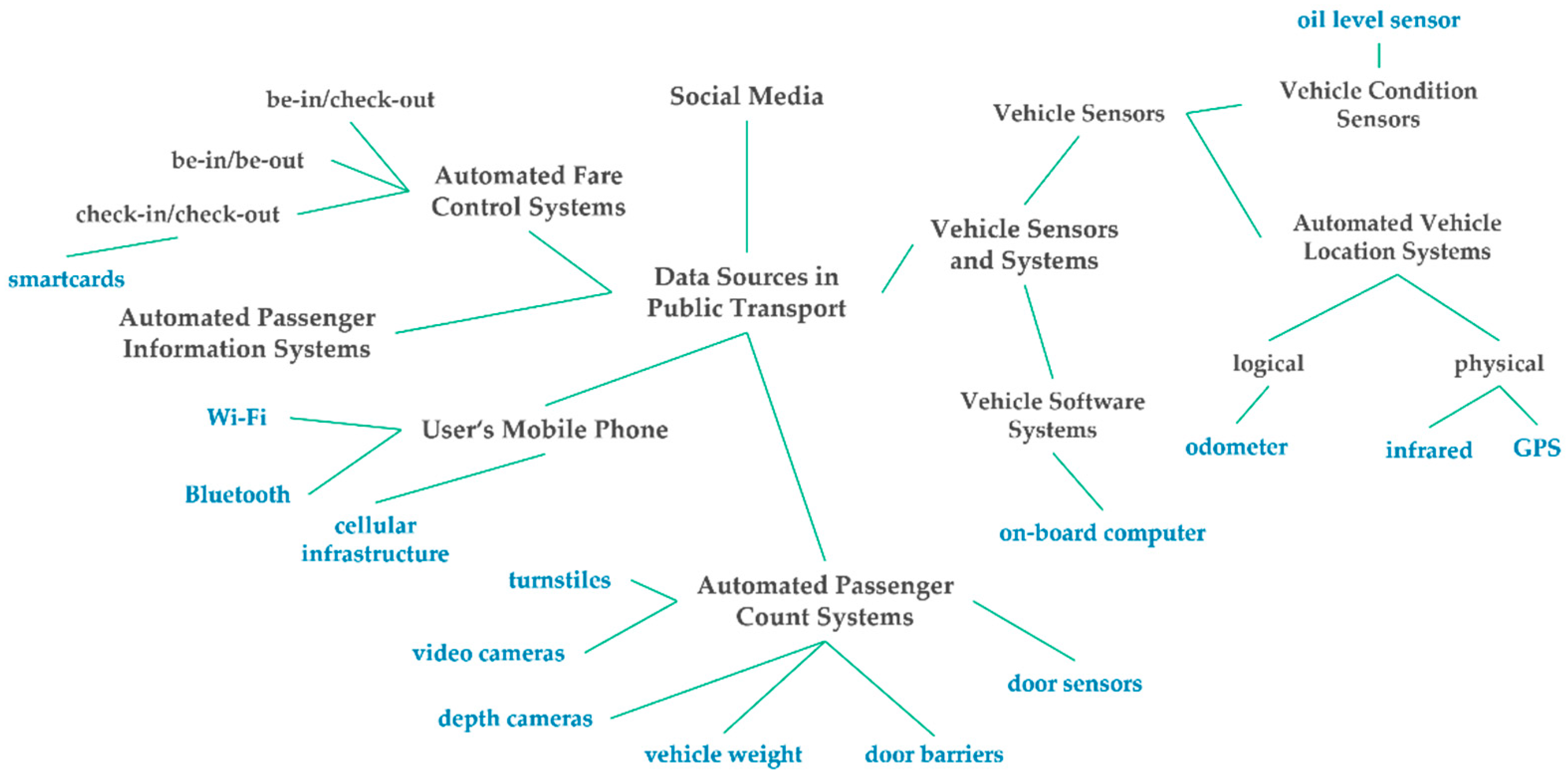
To categorize the data sources, we used the viewpoint of public transport agencies and identified the systems that that produce data as main categories, as displayed in
Figure 1 and listed below:
Automated Fare Control (AFC) Systems
Automated Passenger Count (APC) Systems
Vehicle Sensors and Systems
- ○
Vehicle Sensors
- ■
Automated Vehicle Location (AVL) Systems
- ■
Vehicle Condition Sensors
- ○
Vehicle Software Systems
User’s Mobile Phone
Social Media
Automated Passenger Information (API)
For some of these types of systems, we identified subcategories, such as the physical and logical category of Automated Vehicle Location Systems.
Figure 1 also shows some examples of specific variants regarding the implementation details of these systems. These are also discussed in the following paragraphs.
An Automated Fare Control (AFC) system enables automated ticket sales, ticket validation, and inspection. There are different types of systems. One form is that the passenger actively logs in and out of the system at the beginning and end of the journey (check-in/check-out). In another form, the system automatically registers the start and end of the passenger’s journey, for example, via communication between a radio beacon and the user’s smartphone (be-in/be-out). Furthermore, any combination of both systems can be used (e.g., check-in/be-out). Based on the duration and the start as well as end point of the journey, the fare is determined automatically. An AFC System can be implemented using a wide variety of media. Currently, smartcards seem to be the most common medium. As we observed in all three meta-studies, most of the papers handling AFC data deal with the analysis of data collected by means of smartcards. Using AFC data, one can obtain a good impression of passenger’s actual movement in public transport. If a public transport association uses no Automated Fare Control system, the actual movement of passengers and therefore the real load on a public transport system must be determined another way.
An
Automated Passenger Count (APC) system is a system that automatically records the number of passengers aimed at determining the real load of a public transport system. Several types of APC exist; turnstiles can be used to detect passengers boarding and alighting at stops. This method requires a fully fenced traffic system, which is rare. A rough estimate of the passenger volume can also be achieved by weighing the vehicles [
4]. More accurate passenger counts can be accomplished using infrared or laser barriers on the inside of vehicle doors [
5]. Video and depth cameras can also be used for automatic count passengers [
6].
Public transport vehicles record a wide variety of data. These are in the category Vehicle Sensors and Systems, which is split into the subcategories Vehicle Sensors and Vehicle Software Systems. Data from software systems in a vehicle include data from the on-board computer, the communication module or the passenger information displays, for example. Sometimes, sensor data are logged in vehicle software systems, such as the on-board computer. It can be logged as raw data or already interpreted data and are often complemented with other data, such as the line and stop sequence the vehicle is driving.
Vehicle sensor data can be roughly categorized into two categories. Sensors are used to monitor the condition of the vehicle or to locate the vehicle. Examples for
Vehicle Condition Sensors are sensors for the oil level, or for the condition of the oil filter [
7].
Automated Vehicle Location (AVL) systems are used to determine the location of a vehicle during operation automatically. In public transport, a distinction is made between logical and physical location procedures [
8]. Logical and physical positioning can also be used complementarily. Logical positioning takes advantage of the fact that public transport is usually organized as a regular service. This means that the position, starting from a defined starting point, can be recorded based on the distance traveled and can be logically deduced. The distance traveled can be determined, for example, by means of an odometer via wheel rotation. Physical positioning is possible, for example, via infrared markers at bus stops. These can be registered by vehicles, whereupon the position of the stop can be assigned to the vehicle. Probably the most common form of location determination today is using a satellite navigation system via GPS (Global Positioning System). Relevant for the usage of AVL data is the frequency in which vehicle positions are recorded as well as if and how the vehicle positions are reported in real time. Both properties may significantly vary for different public transport systems and sometimes even within one public transport system, for example, because of differences in software and/or hardware in vehicles of different modes of transport.
Another possible data source for public transport is the
User’s Mobile Phone. Most public transport passengers use a mobile phone, which is why information about the passengers and their movement can be concluded from mobile phone data. Data about or from a mobile phone can be accessed either using the cellular infrastructure, Wi-Fi or Bluetooth. Mobile phone data are, for example, recorded and can be provided by telecommunication companies. By using the triangulation of the measured received signal strength and the signal transmission time between a mobile phone and the base station, the location of a mobile phone device can be determined. The spatial resolution can be improved to a few meters if three or more base stations are within range [
9]. Thus, for example, changes in the location of passengers can be accurately detected. This data source extends beyond the scope of public transport, but can also be analyzed specifically targeting public transport usage. However, the analysis of mobile phone data is often limited due to data protection and licensing problems [
10]. Therefore, it is often difficult for a transport company to obtain these data from telecommunication companies. In this case, the transport operator has the option of using Wi-Fi or Bluetooth sensors as radio beacons. These sensors can detect the passenger’s approximate position by communicating with the passenger’s mobile phone device [
10]. Similar to mobile phone data computed from signal strength, the accuracy can be improved by using multiple sensors in combination with triangulation techniques.
Social Media has also become a data source harvested for public transportation in recent years. For analysis and research, social media networks usually make their data available via application programing interfaces. However, there can be major differences in the extent to which the networks make their data available and at what cost. Since the various social networks all have a similar purpose but can differ greatly in their range of functions and interaction options, the data generated through them are correspondingly diverse. As a result, the data from the various social networks are differently suited for the application areas in public transport, as shown in the literature review of Nikolaidou and Papaioannou [
11]. Their research also indicates that Twitter data are currently the most widely used social media data source in public transportation research.
In addition to the data sources discussed by the above-mentioned meta-studies, we introduced one additional possible source of data in public transportation:
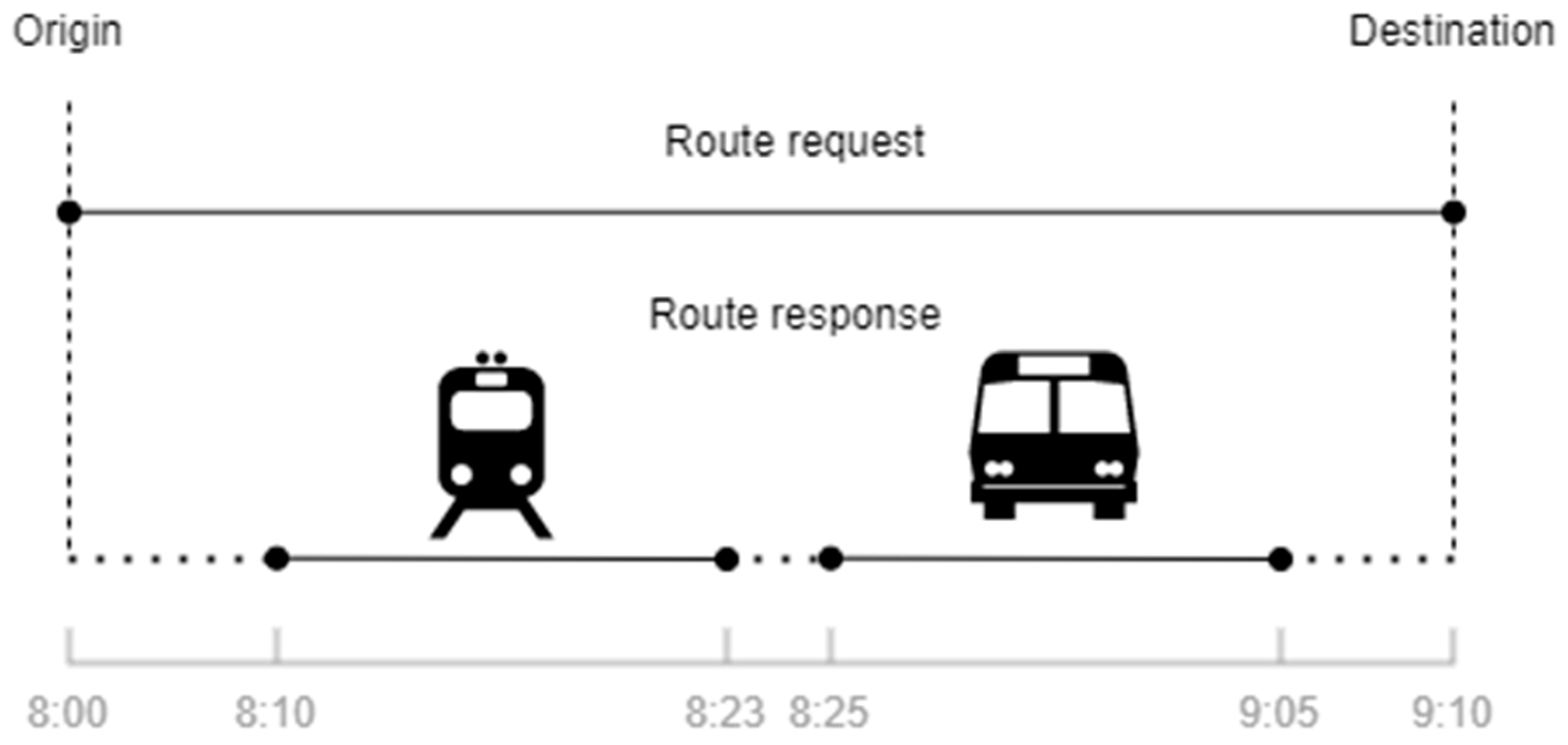
Automated Passenger Information (API). Automated passenger information systems allow passengers to plan their trip and be always well informed about the public transport network and their planned or current journey. A good example for possible data that are generated by API are electronic route planning systems. An electronic route planning system enables travelers to retrieve journey options and information about journeys. For this purpose, the user specifies at least the origin, destination and the desired departure or arrival time of their intended journey. Based on this information, the system can then calculate possible routes and display them to the user. A route planning system does not necessarily have to be limited to one means of transport, but can also include multimodal information. The data that a route planning system stores can be distinguished into two datasets. The first dataset contains the requests of the users to which we further refer as route requests. A route request contains, for example, the requested origin and destination as well as the desired departure or arrival time of the user. A more detailed list of data contained in a route request is given in
Section 4. The second dataset contains the results calculated by the routing system, i.e., the possible connections, based on the user’s entries. We further refer to this dataset as route responses. Typically, several possible routes are found and calculated for each route request. Likewise, a possible route often consists of several legs that the passenger has to cover in order to reach their destination.
Figure 2 shows the difference between route requests and route responses. In this case, one possible route is found that consists of two legs.
3. Use Cases and Related Work
The previous section showed that there is a large variety and quantity of digital data that are generated and can be harvested for data analysis in public transport. Similarly, there are numerous and various use cases that can benefit from a deeper analysis of public transport data. We systematically collected and structured these use cases to understand better the information need and the potential of big data analysis approaches in public transport. For our analysis, we conducted several workshops and discussions with public transport agencies and operators as well as with companies developing several types of software for public transport operation. We organized the emerging use cases in two dimensions and discuss them in this section.
Table 1 shows the result of our use case analysis in two dimensions: time and types of tasks. The timing of data analysis and usage greatly influences the methods that are applicable. The time dimension is organized as follows: data can be analyzed to immediately assess or manage the current situation. Use cases aiming at current events or the current situation require real-time capable methods and infrastructure. Other use cases utilize data analysis for the short-term future, to support decisions for the same or the next day or week. In this case, the analysis is not needed in hard real-time, but still can be time sensitive. Data can also be analyzed for the support of planning in the medium-term future, ranging from weeks or months to up to a year. In public transport, there are also use cases in long-term planning that affect decisions for several years in the future. Those use cases allow the application of time-intensive methods.
In addition to ordering use cases after the time frame, the second dimension addresses the type of tasks that can be supported. For varying application domains, different types of data are needed. This dimension includes monitoring and planning the public transport network, all use cases considering the timetable, applications for public transport vehicles, knowledge about public transport passengers and their behavior and passenger information.
Managing and developing the
public transport network are core tasks of public transport agencies and there are many use cases for data science for tasks concerning the public transport network. Analyzing public transport data using data science methods can support operators in determining and assessing the current situation in their network [
12,
13]. Big data methods can also be used to evaluate the network’s performance by monitoring and analyzing the demand and actual passenger count, delays, and disruptions [
14]. Using historical data, patterns of broken connections can, for example, be analyzed to reveal flaws in the timetable and network plans [
15]. Duty scheduling can also be optimized. Depending on available sensor and other relevant data on infrastructure elements and vehicles, the predictive maintenance of the infrastructure can improve the longevity of these elements [
16,
17,
18,
19].
Looking at the medium-term or long-term future, the planning of lines and overall network planning, including new stations and stops, can be informed by a careful analysis of long-term historical data and a prognosis of demand [
20]. The support of planning also extends to multimodal planning, taking other modalities into account. Approaches analyzing bike sharing exist, for example [
21]. By complementing such an analysis with public transport data on demand and usage, multimodal planning and multimodal passenger information can greatly benefit. Additionally, trip planning services can incorporate knowledge about sharing vehicles and their usage to support multimodal trip planning. On another level, infrastructure planning can also benefit from a deep analysis of sensor data, usage data and predictions of demand, for example.
Several types of analysis can benefit
timetable management and service planning. The detection of delays and disruptions as well as a prediction of their effects in real-time can support rescheduling decisions and mitigating actions [
22]. In some types of events, replacement services must be organized as soon as possible. A prediction of demand can provide guidance for implementing such replacement services [
23]. Since disruptions and to some extent delays are unexpected events, handling those events can benefit from available real-time data [
24]. These use cases also depend on real-time capable methods to react quickly to unexpected events. Predicting demand helps to manage on-demand services more closely and optimize resources, for example, minimizing the number of vehicles that are on call for on-demand transport.
The analysis of broken connections as mentioned above can inform the development of new timetables and a more detailed analysis of the public transport demand can be used to optimize the frequencies of lines. Examining the demand of passengers and their actual public transport usage can be used to plan on-demand services, especially when they are supposed to replace existing services that generate such data.
Malfunctions of
public transport vehicles can be prevented using predictive maintenance, based on vehicle data, either in real-time or in short-time periods [
25,
26,
27]. In the case of electric buses, machine learning analysis can be used to plan and optimize the charging of vehicles [
28,
29,
30]. Vehicle capacity planning can also be supported by the analysis of data on demand and passenger count data.
The core of public transport is to transport
passengers. Yet, very often, not much is known about these passengers. There are some data sources that can be used to gain more knowledge about passengers, their whereabouts, goals, and behavior. Considering real-time analysis, it is an important use case to predict passenger numbers in vehicles or at stops. Especially in times of the COVID-19 pandemic, passengers want to avoid vehicles that are too full, but other than that, full vehicles are also a source of discomfort passengers want to avoid. For operators, vehicles that are often too full imply that vehicle capacity should probably be re-planned. Predicting and estimating passenger numbers can be achieved using big data and machine learning [
31,
32]. Based on similar data, passenger flows can be re-directed, for example, in the case of big events, very full vehicles or, on a smaller scale, to optimize boarding and minimize the time vehicles spend at stops.
Mobility behavior can be modeled based on big data, too [
33,
34,
35]. Specific models for public transport usage can support planning and evaluation, but also can be useful for planning replacement services in the case of disruptions or construction, for example. The analysis of passenger data can also be used to secure connections by analyzing the frequencies and popularity of connections or boarding times [
36,
37,
38,
39]. A prediction of public transport demand specifically can be useful for several usages, from the planning of infrastructure, stops and lines long term to the planning of on-demand services [
12,
13,
40,
41,
42]. Lathia and Capra analyzed smartcard data to measure travel behaviors and enable transport operators to manage incentives for behavior change [
43].
Finally, precise and timely passenger information is crucial for a good public transport experience and therefore to increase the attractiveness of public transport. Big data can help to provide passenger information in real time, complementing trip information with information about vehicle occupancy, providing precise information about delays and their expected development as well as providing timely information about disruptions, including trip alternatives, for example. At the same time, data analysis can provide a basis to personalized passenger information, identifying mobility patterns of user groups and tailoring information to user’s mobility preferences, for example. Using knowledge about the user’s preferences, behavior and trips, critical information can be provided ahead of time.
This discussion of use cases for big data methods on public transport data demonstrates that these methods have the potential to improve public transport in a variety of applications.
4. Applying Data Science Methods to Public Transport Data
In our work, we explored use cases to optimize public transport using data science methods, specifically machine learning.
Table 2 lists all projects, the used datasets and methods as an outline.
In this section, we discuss several of our projects investigating the application of data science methods to public transport data and present our insights.
4.1. Project 1: Visual Analytics for Public Transport
Use Case: Data from Automated Passenger Information systems (API) has not been widely used for data analysis in public transport yet. However, first attempts at analyzing route requests to passenger information systems have shown that route requests correlate with real transport demand [
44]. Passenger behavior has been analyzed using data from passenger information systems, for example, for extreme weather events [
45,
46]. Our goal is to explore the potential of API data further. To understand this potential and to develop a basis for discussion of the data and its potential with domain experts, we first explored visualization and visual analytics. We were interested in how the visual analysis of route requests can support network analysis and the analysis of the public transport demand. Visual analytics have been used successfully for the analysis of public transport data before, for example, using data from public transport vehicles, in an approach by M. Wörner and T. Ertl [
47]. We investigated if insights from visualizing passenger requests can form a basis for further optimization and planning. Another goal was to determine which visualizations are suitable for this type of data for data scientists and for domain experts as well.
Data: As described above, we worked on data from automated passenger information systems. In this case, a dataset of route requests received by the KVV (Karlsruher Verkehrsverbund, the transport association in the Karlsruhe region, Germany) was made available. The period of the data set was between 1 January 2019 and 10 October 2019 and contained over 18 million requests. This is a good example for the scale of the data that are produced in the operation of public transport. Each request contained the information shown in
Table 3.
Methods: We decided to develop an interactive visualization dashboard that allowed the flexible configuration of visualizations. Due to the possible large data volume, our goal was to allow the dashboard to be operated on different screen sizes. For overview, the application should be usable on our display wall using eight curved displays in two rows. Additionally, we implemented several options to select data subsets and to filter the data for each visualization. The application was realized as a web application using Dash [
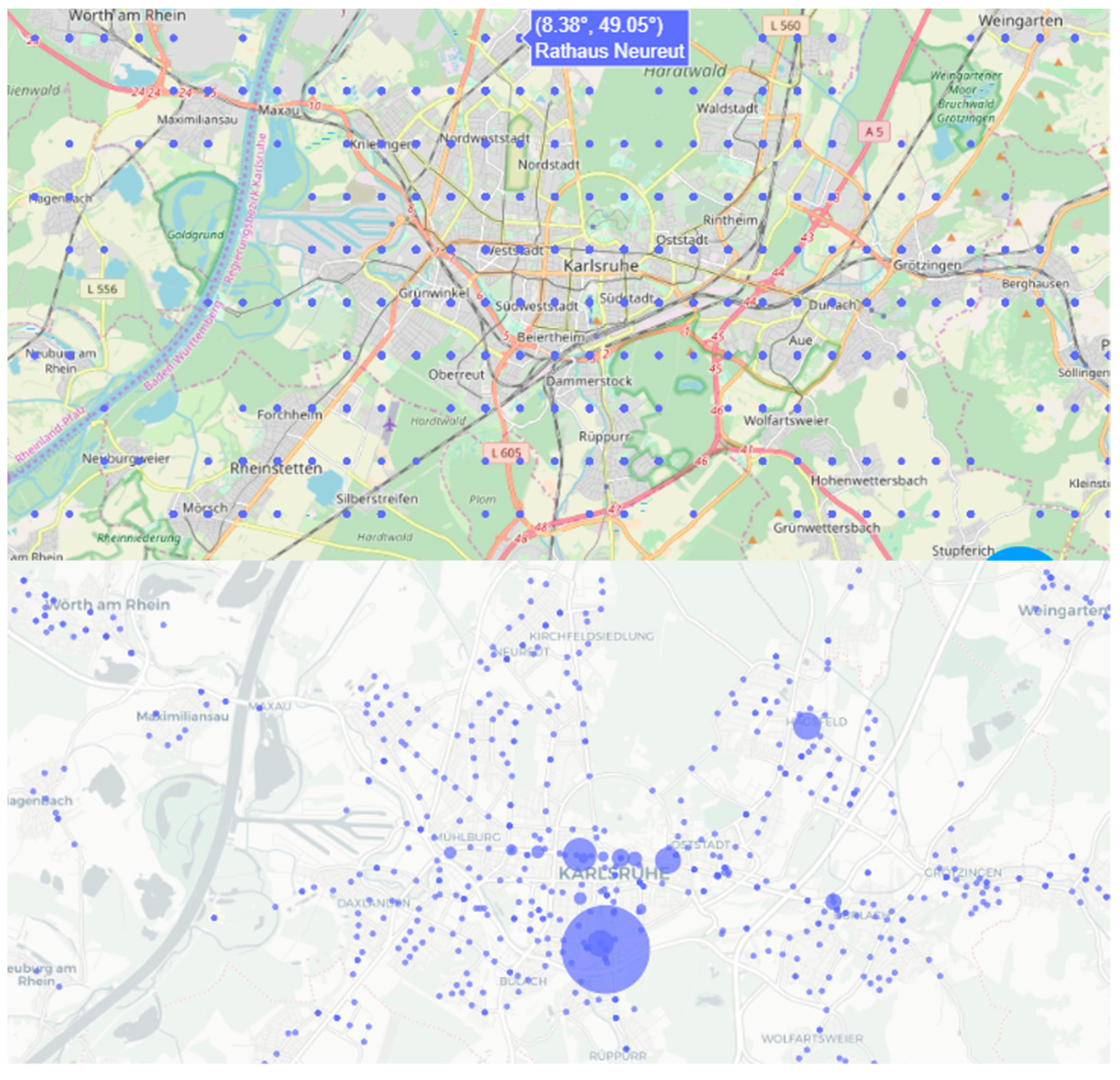
1]. We aimed at visualizing the requests based on their temporal and spatial distribution and therefore started to analyze the temporal and spatial information in the data to determine preprocessing steps. The geographic coordinates of the dataset were given as decimal numbers in the WGS-84 geographic coordinate system. A particularity arises from the fact that, due to the properties of route requests, the current location of a user can be in the query data. Data that contain private information of the user must be handled very carefully to ensure the user’s privacy and data protection. To comply with legal requirements concerning data protection, the public transport association truncated all coordinates to two decimal places, before submitting the data to us for further analysis. This causes a possible deviation of the position by about 1 km. For a geographic analysis in the inner-city area, this accuracy is insufficient. In this work, the data were analyzed on a general and not a personal level. For these two reasons, we revalued the coordinates to at least five decimal places, using additional location information. A total of 93% of the connection searches included stations as sources and/or destinations.
The station IDs were defined by the IFOPT (Identification of Fixed Objects in Public Transport) specification. This circumstance allowed a fast and straightforward mapping with another dataset that contained the stops and their respective more precise coordinates. For the rest of the coordinates, we used the geocoding tool Nominatim [
2] from OpenStreetMap.
Figure 3 displays the result of this approach, showing the spatial distribution of requests and how their precision could be improved. Based on this preprocessed data, we developed an interactive dashboard for the analysis of passenger information data. Several types of analysis and visualizations can be explored on this dashboard. Various settings parameterize the data analysis. The user can choose different temporal settings, e.g., select the time frame or certain days of the week to analyze. In addition, the applications used for the query can also be selected. Individual stations can be selected and thus be examined more closely. The data are visualized in several graphs.
Two pie charts show the distribution of requests among the individual applications and user agents. A bar chart shows the number of requests that mention a point as either the origin or the destination. This chart helps to identify the most requested stops, for example, to choose stops for further analysis. A line chart shows the spatial distribution of the request for the selected time. Another line chart shows the relative frequency of daily requests per weekday, displayed in
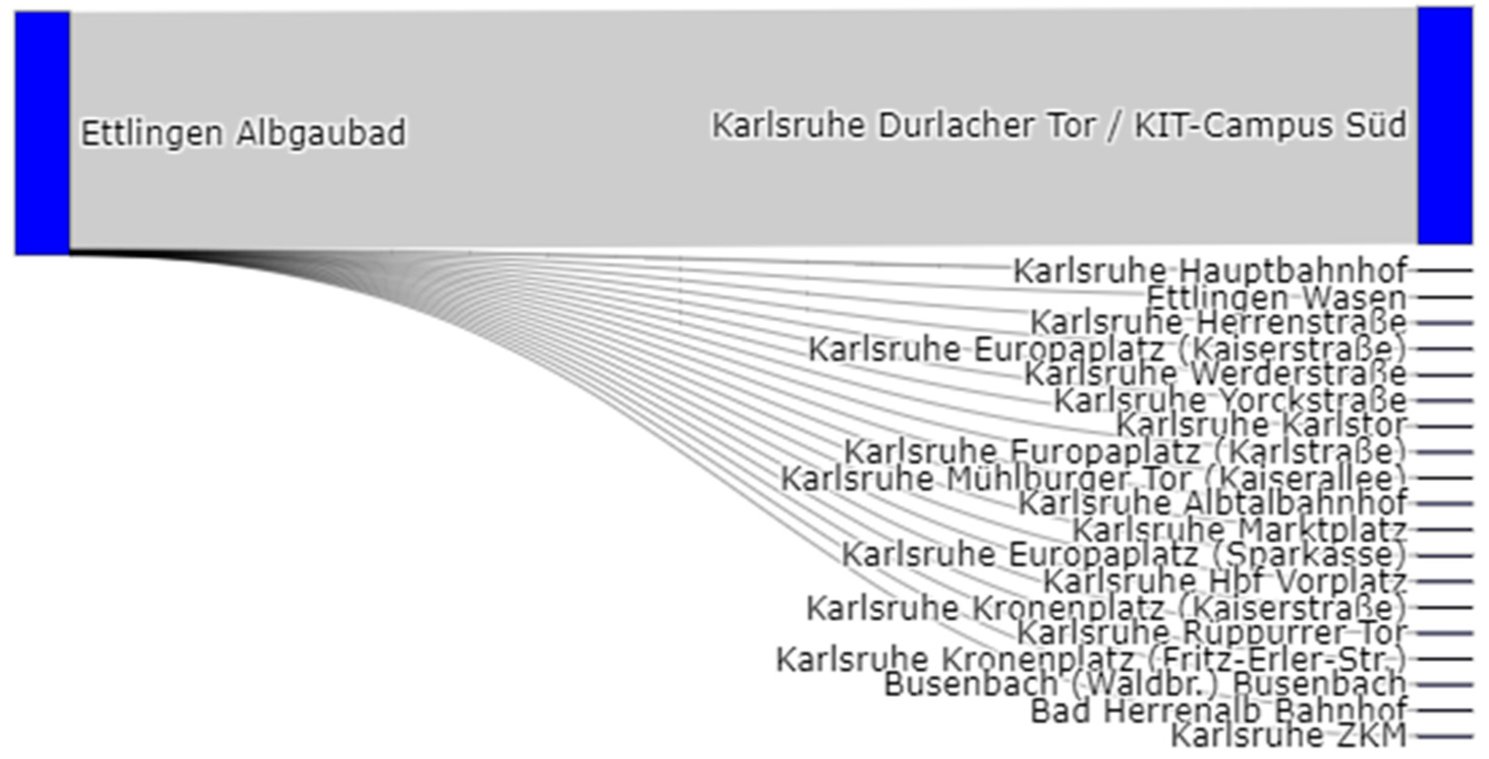
Figure 4. The graph is interactive and allows to select the displayed weekdays and examine the data points more closely. A heat map and a scatter map illustrate the spatial distribution of the requests. The origin-destination relations of the requests are represented by a sankey diagram, shown in Figure 7. Sankey diagrams have been used to analyze public transport data before, for example, by W. Zeng et al. [
48]. The nodes of the sankey digram represent the number of times an origin (left node) or a destination (right node) is given. The length of a node represents the sum of incoming or outgoing connections. The edges connect the origins and destinations with each other and represent the number of connections of each relation by their width. This diagram helps to analyze frequently requested connections and supports a closer analysis of the efficiency of the public transport network.
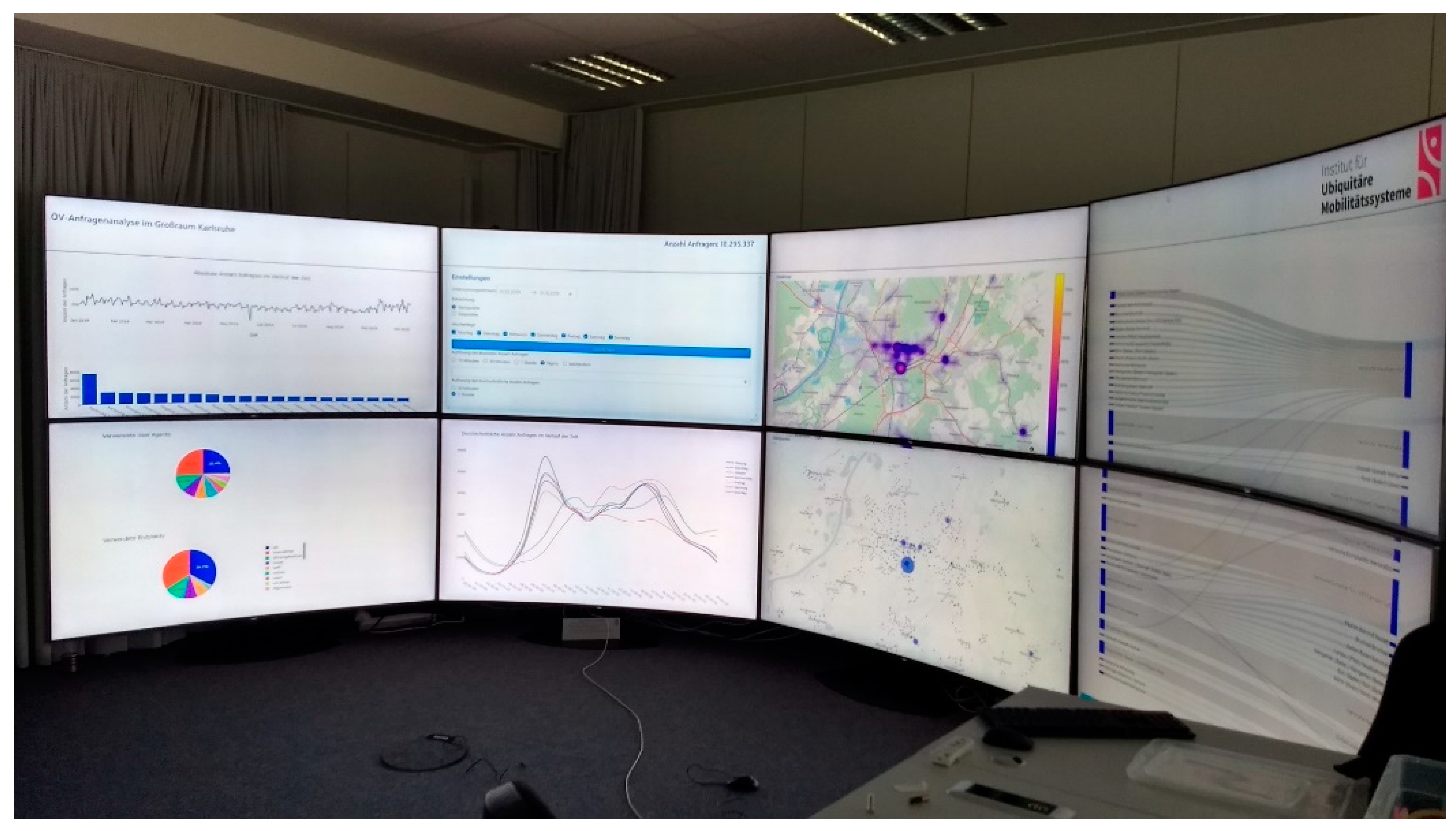
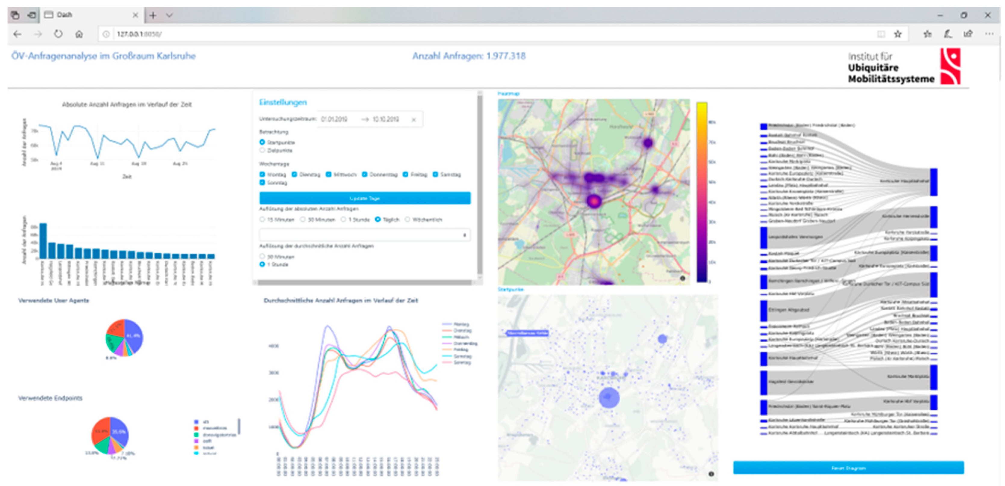
Results and Future Work: The result of this work is a web application dashboard that can be displayed and operated on a display wall using several screens, but can also be used on regular screen sizes.
Figure 5 shows the application on our display wall consisting of eight separate displays. It allows the visualization of large data volumes, utilizing the high resolution of eight separate displays. The dashboard is configurable, so that a user can choose which graphs should be displayed, as shown in
Figure 6. A properties tile in the dashboard can be used to choose the subset of data that should be displayed and to filter the data. Considering our goal to assess, if conclusions about the data and its further analysis can be made based on the visualizations, we found that usage patterns could be revealed in the data.
These usage patterns indicate that the request data reflect the actual demand for public transport. Morning and evening peaks are, for example, clearly visible in the frequency of requests, as can be seen in
Figure 4.
In addition, the peaks at weekends are significantly flatter than on weekdays and are shifted back in time, as they are in analyses of passenger numbers. The usage of trip requests is significantly lower during school and semester breaks due to the absence of school traffic. Such known usage patterns are apparently represented in request data, which links with actual demand. However, the visual analysis also revealed that a considerable amount of the queries are automated queries. These queries, in turn, do not represent a real demand. This is illustrated in
Figure 7, for instance. The figure shows a section of the origin–destination sankey diagram. The top connection was requested many times and more frequently than the others. This most frequent connection leads to the stop of the local university. The second connection in turn leads to the city’s main railway station. Although there is certainly a significant demand for university, the discrepancy between the ratios is clear. Such discrepancies can be explained by automatic requests from bots or other applications that make specific requests in frequent time intervals. Some of these requests can be excluded from analysis by excluding all requests to the endpoint those applications use. However, there are other automated requests in the data that are made by applications and widgets, for example, that are not as frequent and not as easy to identify. Such automated requests distort analyses that focus on public transport demand. To use the data for further analysis or operational decisions, these bot requests must therefore first be filtered. We are currently pursuing several approaches to filter such automated requests.
Our visualization dashboard was tested in exploratory tests by students of transport management and we received positive feedback for our approach towards visual analytics of public transport data. In discussion with representatives from public transport agencies, visualizations proved to be crucial to convey data analysis results to public transport experts, which is why we continue to develop dashboards for visualizations of our data analyses. Future work using this dashboard application includes a user test to measure the usability of this application and a test with representatives from public transport agencies to assess its utility. Based on these tests, we aim at improving the application and iteratively integrating additional data sources.
4.2. Project 2: Analyzing Demand for On-Demand Planning
Use Case: As we saw in our visualization project, data from automated passenger information systems can be used to analyze transportation demand. In a project building on this realization, we wanted to pursue this approach. The objective of this project was therefore to help transportation companies to explore places and times where travel options are not yet sufficient to meet all travel needs. The first goal in this project was to analyze public transport coverage in general, based on API data. Based on such analyses, public transport companies discuss the extension and development of their network. However, apart from adding new railway lines or lines of trams or buses, public transport agencies also consider other types of services to provide travel options to their passengers in places or times that are currently underserved. A second goal of this project therefore was to discover and optimize regions for the implementation of on-demand services based on travel intention and travel behavior. Analyzing travel behavior and demand, for example, using smart card data and exploring similar questions to ours, can be found in works by M. Bagchi and P.R. White or by L.M. Kieu et al., for example [
36,
49].
Data: We used similar data as in the first project. In this case, however, the data were provided by the MVV (Münchner Verkehrs- und Tarifverbund, the transport association for the region of Munich).
Methods: User queries were clustered geographically to find focal points. As described before, the coordinates of a query are blurred to two decimal places to ensure the privacy of users. This already leads to a cluster grid, and each start or end point of a trip request is assigned to a cluster-point in this grid. One problem with the data is that, while route requests are stored, the suggestions a user receives in response to that request are not. To obtain these data, the requests were rerun for the time they were originally run. This has the disadvantage that the historical state of traffic is no longer accurately observed, since requests for a time in the past are processed on timetable data only, not considering real-time data. Then, it was examined how well a trip proposal matched the requested arrival or departure time, if there were any trip proposals at all. This allows an assessment of whether a trip request is well or poorly served by the existing travel services.
Focusing on two study regions, we analyzed the data to support on-demand transport planning in these regions. Heatmaps, time wheels and network spiders were used for visualization. Heatmaps are used for a spatial break down of the request priorities, as displayed in
Figure 8. They are computed both for an entire period of time and for several points in time to display an animated temporal progression. The heatmaps show points where the requested routes are unsatisfactory. A route is unsatisfactory if the relation between travel time and actual trip time, meaning time spent in a vehicle, is greater than a given threshold, in the example 1,1. This indicates poorly coverage, because passengers spend a lot of time waiting for their bus or train. Time wheels, on the other hand, focus more on a temporal classification. In this case, in a view broken down by hours, request priorities can be quickly identified, as shown in
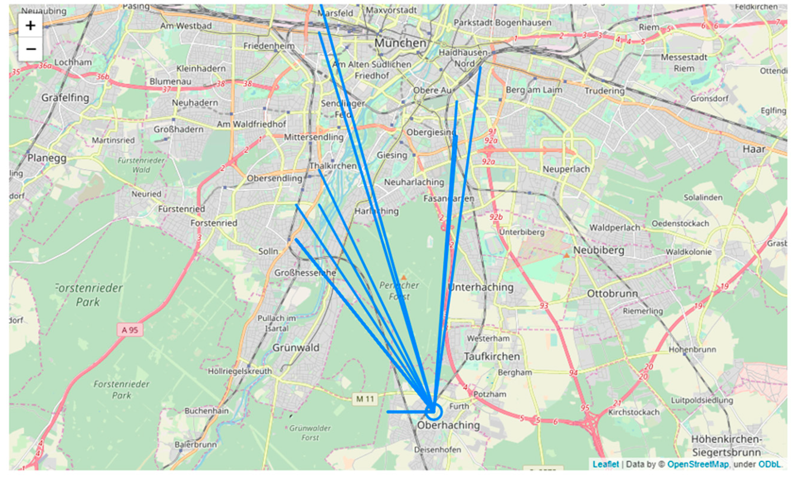
Figure 9. Time wheels were created for an entire region as well as for individual spatial clusters. While these two visualizations only show start and destination points of a route request, these are connected with the network spider. A network spider, as shown in
Figure 10, connects a starting point with various end points. In terms of our data, this means that all destinations (end points) requested from a single location (starting point) are displayed and connected. As an alternative, all request locations to a specific destination could also be displayed. This allows all outgoing and incoming connections to a selected cluster to be displayed. This is intended to make it easier to assess whether the desired connections are only local or more cross-regional.
Results and Future Work: During the evaluation, we identified a need for improvement in places without suburban rail connections. There are requests there that cannot be served at all or only very poorly by the existing public transport system. This means that potential passengers are more likely to choose an individual mode of transportation, provided they have an opportunity to do so. This also means that this individual mode of transport is often used for both the outbound and the return journey, even though there might have been a public transport service on one of the trips. In addition, places that are further away from the core region have poorer connections, which is clearly reflected in the analysis, and is a well-known fact. The analysis therefore needs to provide greater detail and more context to be of use for public transport agencies analyzing more rural regions. In the case of small towns, the problem was that they were not well represented by the usage of the blurred coordinates. At first, we utilized the blurred coordinates for clustering. However, since on-demand transport often involves door-to-door connections, it is necessary to use the most accurate data possible in future work. This is why we will investigate privacy preserving methods that still deliver precise results in future work. Future work will also utilize not only the routing requests but also the recommendations given by the automated passenger information system as historical data to allow for a comparison with current timetables.
4.3. Project 3: Predicting Passenger Numbers in Vehicles
Use Case: The previous project used data from automated passenger information systems for the analysis of travel demand in retrospect, planning for future services. We were also interested, however, in examining the short-term analysis of these data and wanted to see if we also could use route requests to reach conclusions about real-time travel demand. Using our insights from prior research, we wanted to explore if using data from the automated passenger information system could be used for a prediction of passenger numbers in a vehicle at a given time. We also wanted to know if such a prediction could be achieved in real time, based on current request patterns to then be included in passenger information. The prediction of vehicle occupancy has been explored in other works based on different types of data, for example, by Gilles Vandewiele et al. and by J. van Roosmalen [
31,
32].
Data: To enable our research, we needed datasets of observed passenger numbers and the generated route responses for the same period. For this project, we worked with three different transport operators in Germany. Two of the three companies were able to provide us with full passenger count data from their respective APC systems. The third company was not able to obtain permission to release the absolute number of passengers. Only aggregated figures could be provided. Both technical difficulties and data privacy concerns were expressed as the reason. Those aggregated figures were unsuitable for our methodology and were not used further. We therefore could use data from APC systems of two public transport agencies, together with route requests and the recorded route responses of the respective API systems. The APC data were recorded during the same time as the API data.
For every leg in the route response dataset, the following information was given: a proprietary public line identifier, the stop ID and coordinates of the origin and destination stops as well as the planned departure time at the origin stop and the planned arrival time at the destination stop. The APC data contained a line identifier, a stop identifier, a coordinate, a departure time and the recorded number of passengers getting on and off at that stop.
Methods: To investigate whether using route requests and responses can improve the prediction of ridership, we developed multiple machine learning models. Each model was trained and evaluated using two datasets. The first dataset contained all available information. The second dataset did not contain any information about the route responses. In this way, we were able to evaluate the impact of the API information to the accuracy of ridership prediction. The target variable of our prediction was the change in ridership at each station, meaning the difference between boarding and alighting passengers at each station. Using this value, we then calculated the total number of passengers after each station over the course of the journey. We chose Random Forest (RF) and Gradient Boosted Trees (GBT) for our approach. Our literature review showed that these algorithms can perform well in predicting ridership. In related work using datasets similar to ours, these algorithms performed the best [
32,
40,
50]. In addition, with tree-based algorithms, it is possible to obtain an insight into which features are important for the forecast. We hoped this would give us further insights into how important the API data are for the prediction. Before we could apply these algorithms, however, we had to overcome some challenges in matching the passenger count data with the route responses, as the two datasets contained different IDs that had to be matched to each other. Specifically, we had to match each leg proposed to the users with the trip that was operated by the transportation company. None of the datasets used standardized or uniform IDs to designate these trips or legs. In addition, the IDs of the stop identifiers in the two datasets did not match. The standardized IFOPT stop IDs were used for the route response data, but not for the APC data. Instead, proprietary IDs were used there. Furthermore, the public line identifier also differed between the two datasets. Therefore, we had to take the following elaborate approach to be able to link the two datasets. First, we used the coordinates of the stops that were given in both data sets. Using those coordinates, we calculated the nearest matching stops between both datasets. This allowed us to map the stops. Next, the assignment of legs and trips was made using the following criteria:
The line identifier of the trip in the APC data must be the same identifier as the line identifier of the leg in the trip route response.
One stop of the APC trip must correspond to the origin stop of the leg in the route response.
The departure time at this stop must be the same or similar in the APC data as in the route response.
The possible APC trip must also serve the destination after the origin stop of the leg.
Using this method, we successfully merged the two datasets and were able to apply the algorithms to the data. However, the matching process proved to be quite complex and therefore time consuming. We could see at this stage that, given the current data format, a real-time prediction of vehicle occupancy would not be feasible. However, we continued with our work to explore prediction algorithms. In the course of feature engineering, we generated additional features using various aggregation methods. For example, the average number of passengers boarding and alighting for different departure time windows, or how many stops the vehicle had already made before arriving at the current stop. In addition to the data provided by the transport companies, we also integrated weather data, such as mean temperature, wind speed or measured precipitation, for the respective departure day into our models. Weather has been shown to influence public transport usage [
51].
Results and Future Work: Using tree-based algorithms allowed us to analyze which features of the data were used for the prediction by inspecting feature importances. Interestingly, the relative importance of features for the prediction was very similar for the data of the two different public transport companies. This indicates that a model could be reusable for a different public transport company and a different public transport network, without requiring a completely new training phase.
To measure the accuracy of our prediction, we used two criteria. The first criterion was the root-mean-squared error (RMSE) between our prediction of the ridership change and the true observed value. The RMSE was chosen to penalize and prevent high deviations in the forecast more strongly. This criterion was also used to tune the hyperparameter of the machine learning models. For the tuning, we used a five-fold randomized cross validation. The hyperparameters for both the Random Forest model and the Gradient Boosted Trees model were set using a randomized parameter optimization [
52]. We then used several hyperparameter sets. For the n_estimators parameter, we identified a range between 50 and 250 and used a random value in this range for model training. For max_features, we tried to use all features, using max_features = n_features and max_features = sqrt(n_features). For min_samples_split, we used the values of 2, 5 and 10, while for min_samples_leaf, we used 2, 5, 10, 15 and 100 in trainings. For the second accuracy criterion, we used the calculated ridership using the predicted ridership change. This value was compared to the observed ridership at a threshold of 10 passengers. This makes it possible to map a percentage accuracy that, in contrast to the RSME, allows a better comparison with other studies. The results between the datasets of the two transport companies were similar. For reasons of clarity, we only present the results of one of the companies in this paper, as shown in
Table 4.
As can be seen, the results of the RF model were better than those of GBT. The inclusion of API data improves the prediction of total ridership by almost 15%.
Thus, the API data seem to be of great use for forecasting ridership. Nevertheless, we find it difficult to make a definitive assessment of our results. The background is that the study period in this project was during a peak phase of the COVID-19 pandemic. As a result, the observed passenger numbers were significantly lower than in normal operation. The president of the association of German transport companies estimates that the number of public transport passengers in Germany in February 2021 was between 60% and 70% lower than during normal operation [
53]. We assume that this circumstance significantly influences our results. We hope to repeat the study soon under normal conditions. Future research could also investigate the impact of including API data when other complex machine learning models, such as deep neural networks, are used to predict passenger data.
4.4. Project 4: Analyzing Usage of Bike and E-Scooter Sharing
Use Case: An issue of public transport often is the problem of the “last mile”, meaning that passengers need to cover the last trip leg from a stop to their final destination in some way and long distances between stops and final destinations can make people hesitant to use public transport. With the emergence of bike and e-scooter sharing services, these services have often been proposed as a good complement to public transport, because they can enable passengers to cover their last mile comfortably. However, the usage patterns of bike and e-scooter sharing services have not been investigated in relation to public transport yet. In a related work, Albuquerque et al. analyzed bike-sharing data from Lisbon to identify mobility patterns for the optimization of bike-sharing services [
21]. Big data analysis has also been used for fleet management of shared mobility services [
54].
The idea of this project is, therefore, to use historical data from e-scooter and bicycle sharing providers to make predictions about vehicle movements in the near future. On the one hand, knowing patterns in vehicle movements and distribution could result in operational advantages and, on the other hand, it can enable users to plan with greater reliability, since booking in advance is often only possible to a very limited extent. As discussed above, sharing vehicles are a good complement to public transport when it comes to the last mile of a passenger’s trip. However, a certain reliability of the service is needed. With conventional public transport, this is ensured by the timetable. In the case of free-floating sharing vehicles, reliability has to date been based at most on experience. The prediction developed in this project should reflect such experiences.
Data: We collected data of March and April 2021 from two sharing providers in the city of Karlsruhe. The data were retrieved using application programing interfaces from the operators and was requested at minute intervals. Data were stored with an entry for each trip, comprising origin and destination as well as the respective times. However, data from various providers differ in its details. For example, there are differences in the accuracy of the location data of the vehicles. Additionally, available application programing interfaces are difficult to use. There is one provider that, for example, depending on the size of the queried area, only provides geographically summarized data and does not provide the exact vehicle positions. The APIs of the sharing providers Nextbike (Bicycles) and Tier (e-scooter), which were used in the project, provide unique identifiers and precise coordinates and were chosen because of the details in the data. In addition, the sharing systems differ fundamentally, being either station-based or free-floating networks or a combination of these. Nextbike offers a free-floating network that is extended by additional stations and through which the user can reserve a vehicle only 30 min in advance. It is even simpler with the Tier provider. It has a free-floating network without stations or advance booking. This heterogeneity, however, impacts the portability of our approach.
Methods: Two main methods from the field of machine learning were used to answer the questions. One of them was a historic cluster with a k-nearest-neighbor algorithm and the other a convolutional variational autoencoder (CVAE) in combination with a long short-term memory model (LSTM) to predict the network state of sharing providers. The approach of the historical cluster starts a clustering in historical data based on a query with request time and planned trip time. The 3 most similar network states are searched with an KNN (k-nearest neighbor) algorithm, and their development is analyzed. We tried several configurations for the number of nearest neighbors, k, and arrived at k = 3 as a suitable parameter. As a result, a probability value is obtained as to whether vehicles that are available at the time of the request will also be available at the planned time of the trip. The second approach does not consider individual queries, but attempts to predict the development of the entire network. A CVAE is trained in 100 epochs with the help of 6000 historical network states. The autoencoder tries to reduce the network state to two values (dimensions) at a time. The autoencoder tries to reduce the network state to two values at a time. In different iterations of learning, the model is trained to first reduce a network state to two values and then to generate the network state to match the original network state as precisely as possible. In the next step, an LSTM is trained in 120 epochs and 3 Layers with the many two-value pairs of the different time steps. Based on this time series, the LSTM then can predict new values for the future based. With the future values, a network state of the future can now be generated using the CVAE.
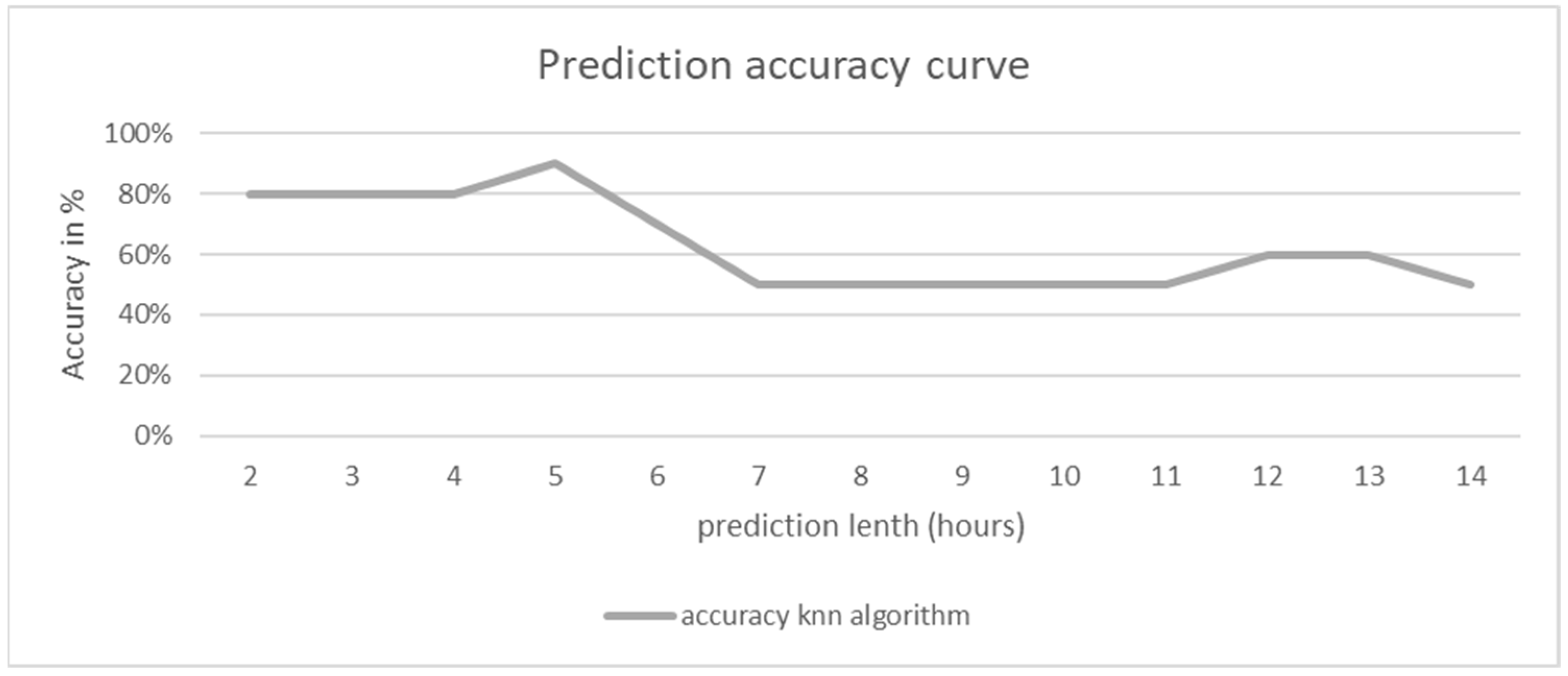
Results and Future Work: Our results show that such a prediction with machine learning methods is possible, but the reliability of the results currently has a broad range, e.g., depending on the prediction length. As shown in the diagram in
Figure 11, the first methodology using the KNN algorithm has an accuracy of about 80% for up to 6 h of prediction. After that, this value quickly drops to about 50% accuracy, which means that good predictions can no longer be made. The value of 80% is also not suitable for reliable planning, but it gives a good indication for further analysis, for example. These values were created with 100 test requests at sample locations in the historical data.
With the second methodology, which should predict the whole network, we had mixed results. The part in which network states are compressed and regenerated with the help of the CVAE works very well after some adjustments. The ELBO (Evidence lower bound) value of the CVAE training is an indication of how well the model is trained. While an upgrade from 10 to 100 epochs in testing improves the model greatly in increase, further upgrades up to 1000 epochs show little improvement. However, the prediction of the compressed values using the LSTM could not yet be sufficiently adapted, so that the results after the prediction and re-generation of a network state appear very blurred and deviate too much from the real development. In this case, an even broader database would contribute to more accurate results, which is part of our future work. In addition, further research should be conducted on the configurations of the prediction models. Prediction models other than the LSTM or particular subsets of it could be tested. In addition, the dimensions of the CVAE could be increased to increase the number of predicted values and thus perhaps achieve better results in the prediction model.
4.5. Project 5: Detecting Anomalies in Vehicle Data
Use Case: In another research project, we analyzed the vehicle data that is recorded by the on-board computers of trams and buses. In contrast to data from passenger information systems and usage data of sharing vehicles, these data are not passenger or usage related. The objective of this project was to use vehicle data for the analysis of public transport operations. The aim was to detect anomalies in the data and consequently in the service performed. For instance, if a vehicle had to take a different route than usual due to a disruption in the traffic network, the data should show this deviation. A retrospective analysis of the data can uncover the frequency of such disruptions, for example, and give insights into underlying problems. Additionally, undiscovered errors of a system component can lead to anomalies in the data. An analysis of the data can uncover unknown problems. Public transport companies are interested in detecting these anomalies to identify faulty components and to analyze vehicle and network performance. Additionally, deviations from the vehicle route are often not recorded on other systems and therefore can not be retraced in retrospect during network evaluations or in network planning. The analysis of GPS-based data for anomalies has been investigated for air traffic by Luis Basora et al. and for individual traffic by Li Cai et al., for example [
55,
56]. For the detection of anomalies in railway infrastructure systems, da Silva Ferreira et al. presented an analysis of unsupervised machine learning methods [
57].
Data: Each on-board computer logs events from the trams’ various system components. The reception of a new GPS coordinate, the opening of the vehicle doors, or whether the driver selected a new destination or a new line, or if the voice radio was activated are entered in the log, for example. The on-board computer that produced the data we analyzed generates one log file per day and per vehicle. The data available for our project were recorded from 4 January 2021 to 20 April 2021. The 472 vehicles generated 139.859 files during this period. Each file has an average size of 5.6 MB. Thus, over 780 GB of data were recorded during our study period. This corresponds to more than 9 billion logged events. This again displays the mass of data that is generated during public transport operation and guided our selection of methods.
Methods: To be able to efficiently manipulate and analyze the data, we used a high-performance computer (HPC). The first errors and anomalies were identified when the data were imported. These were mainly due to faulty software components. To make the data usable, a complex preprocessing had to be carried out, since necessary information, such as coordinates or line designations, had to be extracted first. To detect operational anomalies, we focused on routes. These are represented in the data by the recorded geo-coordinates of the vehicles. Since we had no labeled data available, we chose an unsupervised machine learning approach as a first step for anomaly detection.
We chose the cluster algorithm DBSCAN (Density-Based Spatial Clustering of Applications with Noise) to start our analysis and cluster regular and anomalous trips. We chose the DBSCAN algorithm because it has been used successfully for anomaly detection before [
58]. Additionally, it is not necessary to specify the number of clusters as a parameter. This is a crucial advantage because the number of possible anomalies is unknown. For the calculation of the distances between the trajectories, the Hausdorff distance was chosen based on the literature review by Philippe Besse et al. [
59]. Since this is an unsupervised machine learning problem where there is no ground truth, the tuning of hyperparameters had to be performed by the visual analysis of retrospective results. This was a time-consuming effort and one of the biggest challenges in the entire project.
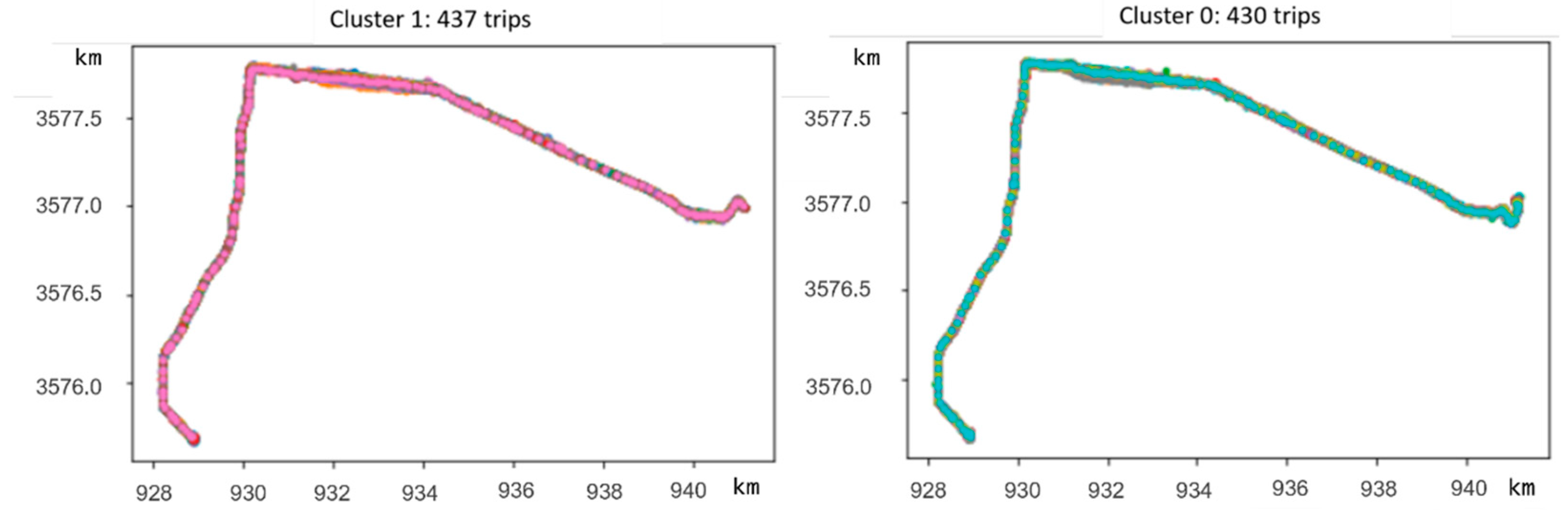
Results and Future Work: We applied the procedure to different subsets of the data, separating data from lines and using data from short time periods.
Figure 12 and
Figure 13 show the results of clustering 1000 trips of a single line, for example. For this clustering result, the parameters were set to the following values: Epsilon = 0.09 and min_samples = 50. Cluster 0 and cluster 1, depicted in
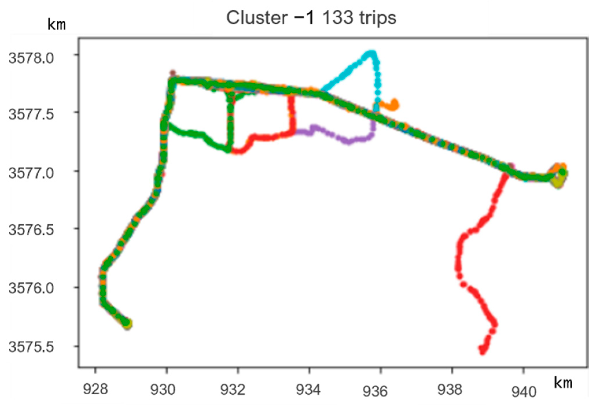
Figure 12, contain regular trips, each in one direction of travel. In the resulting clusters, trips starting from the most eastern stop (in the graph on the right) are distinguished and clustered separately from trips ending on this stop. These trips differ because the vehicle takes a slightly different route on this stop when it is starting from there versus when it is ending the trip there. With a different hyperparameter set, these trips are all clustered in one single cluster. However, in most hyperparameter settings that clustered all regular trips into one cluster, some anomalies were clustered in this cluster as well. We decided to use hyperparameters that distinguish the two types of regular trips and identify anomalies reliably.
Figure 13 shows the cluster containing anomalous trips. In this set, 133 anomalies were identified. Several types of anomalies can be identified using the color coding of trips in
Figure 13, meaning that many anomalies occur repeatedly. These can then be reviewed by domain experts to identify the actual routes of the anomalies and the reasons for the deviations.
For this subset, the clustering procedure works well. Regular trips are assigned to the respective clusters. Anomalies are sorted out and can be considered in further process steps. Limitations arise in the portability of the method between different transport systems and in the use of the entire dataset in contrast to using only subsets. Both traditional trams and tram-trains operate in the public transport network from which we received our data. While trams mainly operate in the inner-city area, tram-train lines also serve regional areas. This results in several differences between the two transport systems, for example, in line length, cycle times and the amount of line variations. This affects the determination of the hyperparameters and the result of the clustering. A tram-train line requires a much higher distance threshold (Epsilon) to achieve accurate results than an inner-city tram line. These results suggest that a division of the data in subsets for each transport system is a reasonable approach. However, we still intend to increase the time periods of the data we use and use data of several lines of trams or, respectively, train-trams together.
We are currently investigating the application of other cluster algorithms, such as HDBSCAN (Hierarchical-DBSCAN), which allows a flexible choice of the distance threshold. Another limitation of our method is the computationally complex calculation of the Hausdorff distance matrix. In the current method, the distance of all trips to each other must be determined. We are currently exploring if we can speed up our calculation by using GPUs rather than CPUs.
We further want to explore the reasons and effects of the identified anomalies. For this, we are currently developing an interactive map that will allow us to study similar journeys and the transport network as a whole, picking up the insights of our visual analytics project.
5. Challenges, Solutions and Lessons Learned
In our data science projects in the field of public transport presented in this paper, we noticed some difficulties handling public transport data and accessing the potential of the data. Some of these difficulties are certainly not unique to the field of public transport and can be encountered in general in the application of data science to big data. Other difficulties, however, occur repeatedly when working with public transport data and point to opportunities to make a difference for the future of data analysis in public transport by addressing them.
In this section, we discuss these difficulties, what their reasons might be and how they can be mitigated.
For scientists, it is often difficult to obtain and work with suitable datasets from the public transport sector due to a lack of available datasets. From the point of view of transport companies, the data are often highly sensitive. In most cases, transport companies are in close competition with each other. In this context, data, such as passenger count data, can provide an unfair competitive advantage for competitors. This in turn means that transport companies are often reluctant to make such data available to researchers or even the public, by implementing an open data policy. Part of the solution may be laws and policies that encourage transport operators to share their data and adhering to open data policies. In public institutions, such guidelines already exist, for example, the E.U. Open Data Directive, or laws, such as the Open-Data-Law in Germany. It is conceivable to extend these guidelines and laws to transport companies, which are often already in public hands or subsidized by public funds. This was implemented, for example, in Germany last year with the adoption of the second Open Data Act. Some public transport agencies have already implemented Open Data policies on their own in recent years, although the extent of the data they provide under these policies is quite different.
In turn, data that would allow to create movement profiles of public transport passengers or allow to identify them, for example, is highly sensitive and should be and remain protected. At the same time, some anonymization measures can obstruct the application of data science methods and prevent meaningful analysis, as we observed in our own work. In order to address this challenge, it is essential to investigate and apply anonymization and privacy preserving measures that are compatible with the chosen data science methods, such as those reported by Kallista Bonawitz et al., for example [
60]. There are also methods specifically for spatiotemporal trajectory data that address the need to analyze location data, but preserve the privacy of the users, as proposed by Sina Shaham et al., for example [
61]. As the adaptation of data science methods for public transport data is currently in its early stages, public transport agencies as data custodians are still beginning to understand the management of their data. Applying privacy preserving methods requires a deep understanding not only of promising approaches towards the data, but also the management of the data itself, which is currently still developing in the public transport domain. Therefore, it is an important goal to deepen this understanding and to work towards privacy preserving data management as a collaborative goal of public transport agencies and researchers.
Often, access to relevant data to pursue a specific use case is obstructed due to organizational obstacles. Data sources are managed by different departments of the public transport association and, as described above, a unified data management approach that aims at utilizing these data is, at best, in its very early stages. An essential first step for initiating organizational change towards such a unified data management is the realization of the potential lying in the data. Public transport agencies are just now realizing how data-driven optimization could benefit the modernization and advancement of public transport. Exploring, clarifying, and explaining this potential has been one of our core goals with the pursuit of the projects described in this paper.
Another hurdle for data analysis in public transport is the variety of different identifiers that are used in public transport data. Part of this problem is that the process of defining consistent identifiers is time consuming and labor intensive and it requires cooperation between different public transport providers and software companies. In the field of public transport, this is even more true due to the large number of companies, system components, and the associated large number of stakeholders. Moreover, transport companies often operate beyond the borders of cities, districts, states, and countries. This further complicates the design of standards. Another part of the problem is that, while there are standards for some of these identifiers, they are often not consistently implemented. The planning and operation of the public transport network requires a variety of systems and components that were developed and deployed for specific tasks, but have evolved to support additional tasks and to provide new interfaces, extending their application domain. Public transport agencies often operate legacy systems using outdated data formats. Therefore, some of the system components in public transport use the developed standards for information exchange between systems, but others do not. It is often hard to upgrade the different systems to use the standards. Possible reasons for this are that it would either interrupt operations, be costly, or the software manufacturer has not yet implemented the standards. Stronger subsidies in public passenger transport focusing on unlocking the potential of public transport data to develop a modern sustainable public transport could certainly make it easier for transport and partner companies to upgrade the system to the current standards.
Mappings between these diverse identifiers are specific and tailored solutions, since every public transport operator has a different system setup and the variety of implemented data formats therefore is very high. This obstructs the development of general solutions and mappings and results in relatively expensive, not easily portable preprocessing for the application of machine learning or big data methods. Additionally, such mappings are often time and resource consuming and impede the development of real-time-enabled solutions. A unification of identifiers and usage of standards could improve the usability of public transport data and advance the field towards real-time capable solutions. Meanwhile, mapping tables can be clumsy, but effective short-term solutions for some of these problems.
Many effects that manifest themselves during the data analysis need to be interpreted by domain experts. One example is the identification of bot requests in our analysis of route requests. The experts that manage and maintain the IT infrastructure of a public transport provider have a deep knowledge of their data and systems and their support is needed to develop preprocessing routines for the data efficiently. In the same way, domain experts that know the public transport network and operations are essential in interpreting analysis results in every stage of the analysis, supporting the decision of which approaches to pursue further, but also utilizing the final analysis results for optimization. In addition to a thorough requirement analysis to specify the requirements for a certain use case, these experts should be integrated in the development process. Developing suitable visualizations is vital for this integration to succeed. Especially for public transport data analysis, we observed that visualizations are essential, but also need to be developed carefully, to be understandable by domain experts. We found that interactive visualizations are especially helpful to access multi-dimensional data. We therefore will continue to research suitable visualizations and interactions for public transport data analysis.
6. Summary and Outlook
The progressing digitization of public transport and the vast amount of data generated in public transport allows rich data analysis and the application of a variety of methods, ranging from visualization to machine learning, to advance the understanding of public transport and to develop a foundation for data-driven optimization. For public transport to fulfill its role in a sustainable mobility, the potential for optimization that lies in utilizing public transport data should be unlocked. As we showed in this paper, there are several different data sources in public transport and a variety of use cases that are worthwhile to explore. However, the current data formats and policies around data usage can complicate data analysis for public transport. The implementation of unifying standards and the continuous modernization of public transport infrastructure can mitigate this problem. Open Data policies—in laws or organizational policies—can help to spark a wide range of research and advance the knowledge about data analysis in public transport as well as raise awareness of the potential that lies in the data. Some projects towards unified data standards, open data policies and consistent data management have already been launched, but these initiatives should be intensified and accelerated. Key to this is to broaden the understanding of the potential of public transport data and to demonstrate the benefits of data analysis. In our opinion, it is highly beneficial to investigate further the visual analytics of public transport data and of data analysis results. High quality visualizations are often complex to develop, but they contribute greatly to the understanding between data scientists and domain experts. We therefore argue that a toolbox of visualization tools, specifically for transport and mobility data, would greatly simplify the implementation of interdisciplinary analysis projects for mobility data. We are further developing our visualization dashboard presented in
Section 4.1 to include additional visualizations and data sources. User tests of the dashboard are planned to improve usability and interaction. Future work on our project about travel demand analysis presented in
Section 4.2 involves privacy preserving methods for handling request data that enables us to use position data in user requests in a sensitive way. We hope to build on results from this line of work in several other projects planned at this time. For the analysis of travel demand, we are looking to join our insights from this project and our project on sharing services, described in
Section 4.4. We are interested in investigating which methods could expand knowledge on travel demands and behavior when data from several data sources and potentially several mobility services are joined. A worthwhile objective would be the prediction of travel demand for several types of transport modes. For the prediction of passenger numbers in vehicles, as described in
Section 4.3, we look forward to resuming our efforts using data from a non-COVID-19 time and to compare our findings for both datasets. Additionally, we plan to use deep learning approaches to explore the problem of predicting passenger numbers from route requests of passenger information systems. The results of our anomaly detection project (
Section 4.5) show the necessity to involve domain experts in the interpretation of analysis results. We therefore plan to advance this project further by including these results in our visualization dashboard. We would like to implement an interactive visualization of the clustering results to enable domain experts to classify the detected anomalies further. The labeled data generated in such a step should be a basis for future work on applying supervised learning methods to pursue anomaly identification.
The projects presented in this paper are of an explorative nature, trying to illustrate the potential of public transport data and challenges in this field of research. We hope to encourage a discussion about data management and data analysis in the public transport domain and to share our experiences and findings with the research community to discuss suitable methods and approaches. We intend to pursue such projects further to eventually help to pave the way for data-driven optimization for sustainable public transport.


