Exergoeconomics as a Cost-Accounting Method in Thermal Grids with the Presence of Renewable Energy Producers

Abstract

Thermal grids are efficient, reliable, and sustainable technologies for satisfying the thermal demands of buildings. The capability to operate at a low temperature allows not only for the integration of heat produced by renewable energy sources but also for the storage of surplus electricity from the grid via “power to heat” technologies. Besides, in the future, heat consumers are expected to behave increasingly as “prosumers”, supplying in some periods heat produced by renewable energy plants on site. In this scenario, it is important to propose a method for the cost allocation among producers connected to the grid. In this regard, this paper proposes Exergoeconomics as a possible tool for rational cost assignment. To show the capabilities of the method, some operating scenarios are compared for a cluster of five buildings of the tertiary sector interconnected by a thermal grid. Based on exergoeconomic indicators, such as the exergy and exergoeconomic unit costs, insights into the cost formation process of the heat consumed by users are provided. Sensitivity analyses of heat unit cost to design and operating variables are also performed. Results show that in the presence of distributed producers, the heat unit cost could be approximately 33% lower than in the case of centralized production, due to the lower amount of irreversibility generated. Capital investment accounts for 20–28% of the heat unit cost.

1. Introduction

It is estimated that in the European Union (EU), space heating accounts for nearly 64% of final energy consumption in the residential sector [1]. The adoption of energy-saving measures and the exploitation of renewable energy sources (RES) are the main routes for reducing the environmental impacts of this sector [2]. Among the available technologies, district heating and cooling (DHC) networks are well-established systems that satisfy the thermal demands of buildings efficiently and reliably [3].

District Heating (DH) networks are widely adopted in Northern, Central, and Eastern Europe [4]. Fahl et al. [5] estimated that in Europe DH covers about 25% of residential heating demand. Nowadays, DH systems consist of centralized power stations that supply pressurized hot water or steam via pipes to urban areas [4]. Such systems are characterized by significant heat losses, and they could not allow for the integration of low-temperature heat coming from renewable energies sources or industrial processes [3]. Typical heat sources to DH systems are Combined Heat and Power (CHP) plants, fueled via fossil fuel, municipal waste [6], or biomasses [7]. Colmenar-Santos et al. [8] projected that the use of waste heat available from power plants for supplying DH networks in the EU would lead to a primary energy saving of about 15%. Regarding District Cooling (DC) systems, the main drawback lies in the small temperature difference between the water supply and return, which leads to high flow rates and pumping costs [4].

It is widely recognized that DHC networks will play a key role in the achievement of 100% renewable energy communities [9]. First, they could help solve issues related to electricity surplus from RES, which is responsible for electric grid instability. More specifically, the electricity surplus can be supplied or stored in DHC networks after being converted into heat or cold via power-to-heat/cold technologies [10]. This concept is one of the pillars of “smart energy systems”, which are currently under investigation [11]. 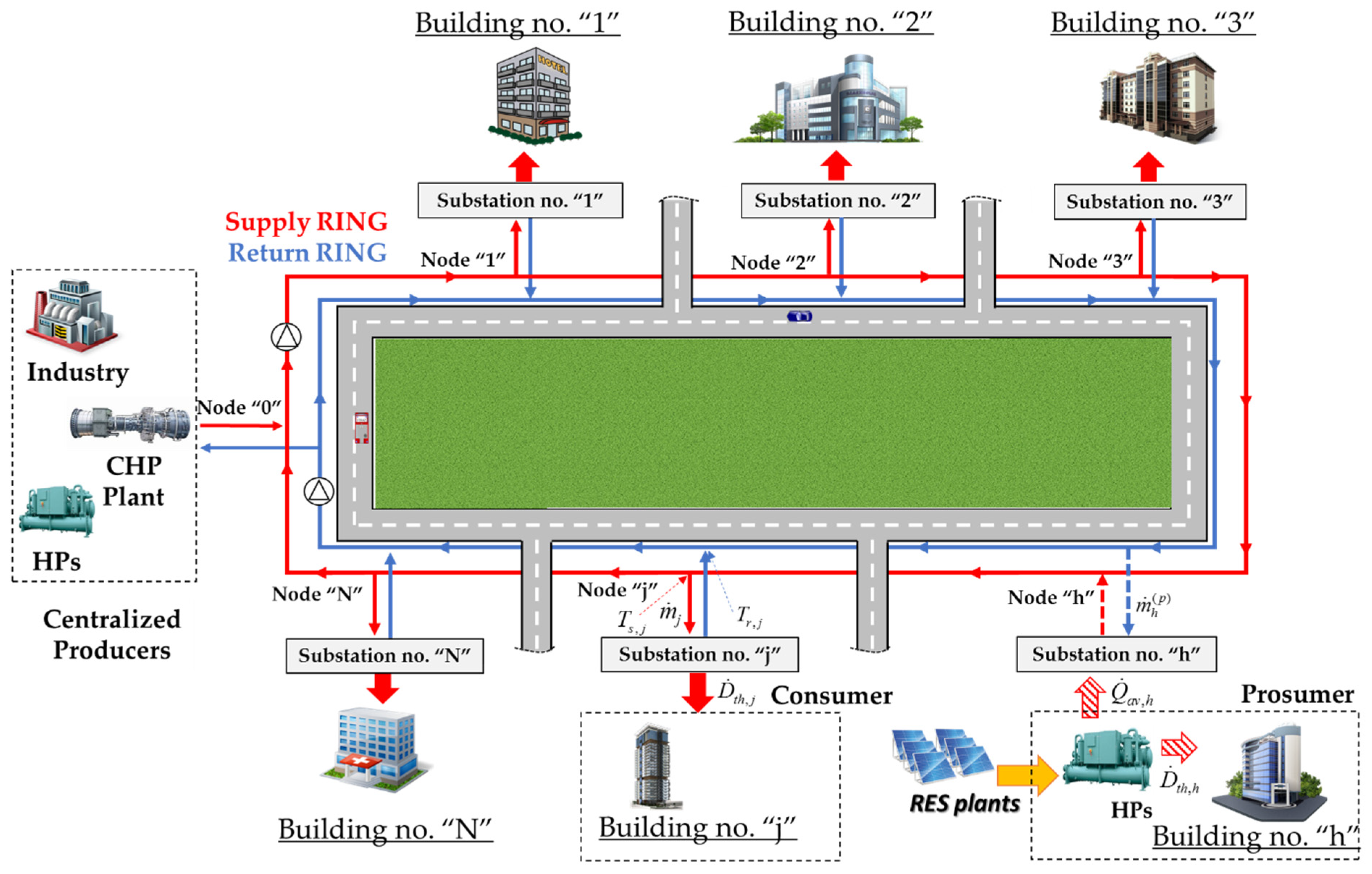Secondly, the reduction of operating temperature will allow for the integration of low-temperature heat from RES, the integration of waste heat available from industry or data centers, and the reduction of distribution heat losses [12,13]. Regarding heat production, similarly to the electricity grid, a typical heat consumer connected to a DH network could become, usually for some hours in a day, a producer supplying any surplus heat produced by RES plants installed on site. Such a customer is not more classified as “only-consumer”, but it is a “consumer-producer”, briefly indicated as a “prosumer” [14]. The DHC systems whose features could enable the transition to renewable energy communities are indicated as 4th [3] and 5th generation [12]. In general, these two generations are featured by a progressive reduction of the operating temperature of the network. Indeed, from an average of 60 °C for the 4th generation network [3], the temperature is reduced to 25 °C (almost near to the ambient temperature) for the 5th one [12].

During these years, some models were proposed to simulate the operation of DH systems based on graph theory [15], electrical circuit analogy [16], and agent-based model [17]. Allegrini et al. [18] performed a review and comparison of simulation tools for DHC networks, comparing their capabilities and accuracy. The results indicate that EnergyPlus, ESP-r, TRNSYS, and Modelica have the best capabilities of simulating DHC networks. Other papers focused on optimization techniques for improving the energy, economic, and environmental performance of these systems [19,20,21]. Some studies focused on cost assessment and allocation in DH systems. Gudmundsson et al. [22] evaluated the Levelized Cost of Heat (LCOH) for the 4th and 5th DH systems for two districts located in Denmark and Spain, respectively. Results revealed that 4th DH networks led to greater economic benefits compared to 5th DH networks. Sun et al. [23] performed a marginal cost analysis for DH systems. The authors calculated the marginal costs for heat production in a Swedish DH plant using different allocation criteria. They found that the marginal cost could better reflect, compared to the real heat price model, the actual increase of variable heat production costs while accounting for the heat production technology adopted. Alajmi and Zedam [24] performed a life cycle cost analysis for comparing DC systems, rooftop units, and variable refrigerant flow as the cooling systems of buildings in hot climates. The study indicated that DC systems are the most cost-effective option over a life cycle of 24 years. Tian et al. [25] performed thermo-economic optimization of a solar-based DH plant, fueled with flat plate and parabolic trough collectors. The authors found that the LCOH can be reduced by 5–9% using solar collectors in the district heating network. Dorotić et al. [26] used a specific allocation criterion named “electric power loss due to heat production” for allocating sustained cost and emitted carbon dioxide (CO₂) on the heat and electricity produced in cogeneration units serving a DH system. Li et al. [27] presented a dynamic price model based on LCOH for district heating. The authors compared three criteria to allocate the fuel cost to the variable costs of heat production, based on energy, exergy, and the market price of electricity. Millar et al. [28] showed that a 5th DH network achieved a 69% reduction in LCOH compared to an electrified non-shared energy system. For instance, Fahlén and Ahlgren [29] focused their analysis on other types of costs, rigorously accounting for external costs for the DH network in Gothenburg, Sweden.

Although the cited papers have addressed the cost analysis of DHC networks, there is still the need for the formulation of proper cost allocation strategies that could support the design and management of these complex systems, while accounting for the innovative aspects in their operation. Indeed, the provision of proper cost-accounting methods could be an effective instrument to promote the sustainable development of new generations of DHC networks. For instance, in the presence of prosumers, it should be considered that heat could be generated at different temperatures. In such cases, these flows will have a different thermodynamic quality, and a rational criterion should pay back producers not only for the amount of heat supplied but also for its quality. In addition, the unit cost of the heat should account for the mix of sources used in its production, the inefficiency that occurred in the distribution network and users’ substations, the incidence of the capital investment, and so on. It follows that a systematic procedure capable of reflecting all these aspects is required when decisions regarding the design and operation of these systems must be taken.

In this work, Exergoeconomics is proposed as a tool for supporting cost accounting procedures in DH networks. This method assumes the exergy content of products as a rational basis for allocating the costs sustained for their production instead of energy [30]. More specifically, the exergoeconomic unit cost of an energy flow or a stream of matter quantifies the monetary expenses that are sustained to produce a unit of exergy of the given product in terms of equipment purchase and operation. Costs are calculated based on a rigorous accounting of all the exergy destructions that occurred along the production process to obtain the examined stream or energy flow. The more inefficient the components involved, the higher the amount of irreversibility “charged” on it and, consequently, its cost. By a systematic procedure [31], the cost formation process of each product of a process is identified and costs are consequently allocated. These capabilities can provide additional insights in the analysis of DHC systems compared to the conventional thermo-economic method where energy is selected as a basis for cost allocation (instead of exergy). Indeed, being energy a conservative quantity, it does not account for the effects of thermodynamic inefficiencies occurring along the productive process (e.g., during production, distribution, and conversion within users‘ substation) on the unit cost of the consumed heat. In other studies [30,31,32,33], it was demonstrated that thermodynamic inefficiencies could highly affect the unit cost of the product(s) of energy systems. Then, to reduce heat unit cost, it could be helpful to rely on a method that accounts for all these aspects. Moreover, if energy was assumed as a basis for cost allocation, producers would be paid back only for the amount of the heat supplied to the network, regardless of its quality (which, is highly dependent on temperature). Conversely, it was proven that the use of exergy could help to solve issues when allocating costs in energy systems characterized by flows with different quality [32,33,34,35]. Finally, through Exergoeconomics, a more thermodynamically sound and cost-effective design and operation of DHC networks could be achieved.

Some papers were specifically focused on applications of Exergoeconomics to DHC networks. Ozgener et al. [36] performed an exergoeconomic analysis of geothermal-based DH systems operated in Turkey. The authors used exergoeconomic indicators to quantify the relation between the reduction of exergy destruction and the increase in capital costs. Lozano et al. [37] performed an exergoeconomic analysis of central solar heating plants coupled with seasonal storage to serve the demand of 500 dwellings in Zaragoza (Spain). The analysis provided insights into the process of cost formation, in terms of interaction between the different components of the examined system. Erdeweghe et al. [38] analyzed different cost metrics for CHP plants serving DH systems. The authors recommended the use of the “Levelized Cost of Exergy” as a cost metric in renewable energy-based CHP plants. Oktay and Dincer [39] performed an exergoeconomic analysis of the Gonen geothermal district heating. The analysis highlighted that the exergy destructions primarily occur because of losses in the cooled geothermal water injected back into the reservoir, with further losses in the pumps, heat exchangers, and pipelines. Tan and Keçebas [40] performed thermodynamic and economic analyses of a real geothermal district heating system using advanced exergy-based methods. Splitting exergy destruction into endogenous/exogenous and unavoidable/avoidable parts revealed that pumps have the highest improvement and cost-saving potential. Meesenburg et al. [41] performed a dynamic exergoeconomic analysis of a large-scale heat pump (HP) used for ancillary systems in a district heating system located in Copenhagen. The analysis revealed that although the unit increased demand flexibility, it also resulted in higher exergy destruction, mainly due to the heat losses during storage and the need to reheat the fluid via an electric heater. Salehi et al. [42] relied on exergoeconomic analysis to monitor the variation of the cost of heat produced via solar-assisted absorption heat pumps for space heating for a DH system in Iran. Čož et al. [43] performed an exergoeconomic optimization of a DC network. The study tried to determine optimal values for the tube diameters and insulation thicknesses of a 1000-m-long supply line, accounting for the different cooling capacities provided. Calise et al. [44] performed an exergoeconomic analysis of a hybrid solar–geothermal polygeneration system producing electricity, heat/cold, and desalted water for a community. Results revealed that the exergy efficiency varies between 40–50% in the winter and 16–20% in the summer. The electricity and freshwater costs vary between 15–17 and 57–60 c€/kWh_ex, respectively, while chilled and hot water costs vary between 18.6–18.9 and 1.6–1.7 c€/kWh_ex. Coss et al. [45] combined exergetic cost analysis with graph net theory and applied the method to a DH network in Turin (Italy). The approach provided detailed insights into the exergy cost formation during transient operating conditions. Bagdanavicius and Jenkins [46] investigated the potential for using the heat generated during the compression stage of a compressed air energy storage system, proposing an exergoeconomic analysis to allocate costs on the produced electricity and heat. Verda et al. [34] showed the potential of Exergoeconomics for cost allocation in DH networks using two applications: third-party access of multiple producers and the connection of buildings equipped with low-temperature heating systems to the district heating network. In the first case, the results showed that using cost allocation on an exergy basis, the heat unit cost could account for the different temperatures of the heat provided by different producers. In addition, in the case of low-temperature heating systems, the variation of the unit cost of heat was assessed while considering the possible connection to the supply or return side of the DH network.

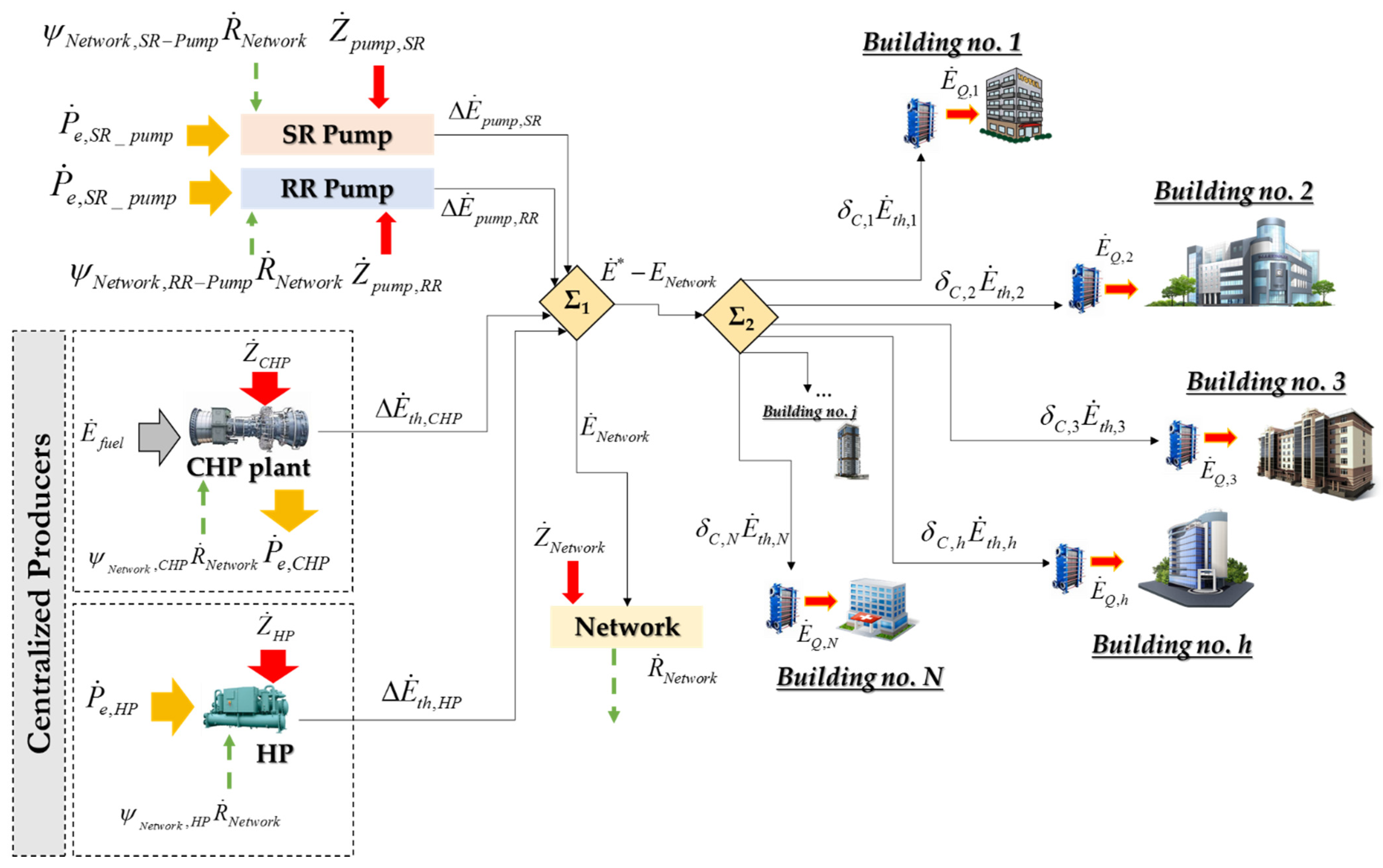
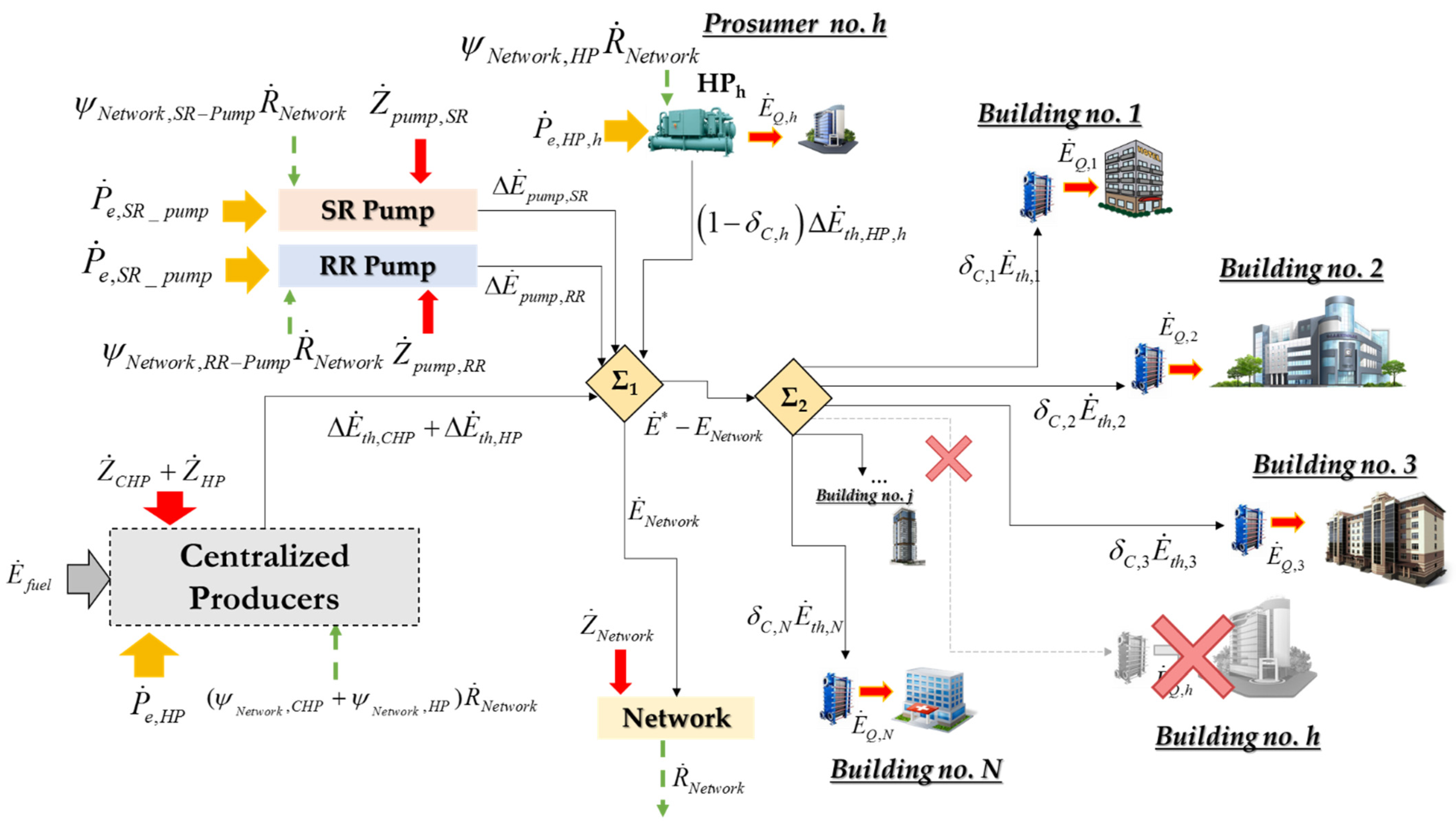
From the previous literature review, it follows that although several exergoeconomic analyses of DHC networks have been performed, many studies mainly focused on the effects on global exergy destruction and cost variation in the case of thermal RES exploitation, not providing details on the cost formation process of the heat supplied to users. Other papers, conversely, aimed at the minimization of the unit exergoeconomic cost of the distributed heat while considering only centralized producers. In the framework of the emerging low- and very-low temperature networks with the presence of multiple producers, a thermodynamic-sound and easy-to-handle cost allocation criterion could be very helpful for evaluating design options and comparing management strategies. Relying on Exergoeconomics, the present aims at developing a method capable to reflect the shares of capital and operational costs, while accounting by ad-hoc exergoeconomic indicators for (i) the thermodynamic inefficiencies occurring along the heat production and distribution process, including heat losses and pressure drop; (ii) the different thermodynamic quality of heat flows supplied to the grid; (iii) the inefficiencies occurring due to part-load operation of production units, in case of reduced thermal demand; (iv) the benefits due to exploitation of RES or the presence of energy prosumers; and (v) the possibility to allocate different capital costs in hours characterized by high or low aggregate demand from the cluster. Moreover, a novel exergoeconomic model of a thermal grid is proposed, valid not only in the case of centralized producers but also in the presence of distributed prosumers. A detailed description of the rationale followed in the development of the model is provided. Details on cost distribution among components are also given, to allow for a thorough understanding of the functional interactions among components. As will be shown, the model can be easily coupled with the physical model of the network, and it is flexible to perform sensitivity analyses on design and operating variables. To illustrate the potential of the method, a cluster of five buildings of the tertiary sectors is assumed as a case study. In particular, a ring-shaped network with centralized fossil-fuelled CHP is considered as the Base Case, and two alternative scenarios characterized by the presence of centralized or distributed RES producers are compared.

2. Method and Materials

To ensure the self-consistency of the present study, some insights into exergoeconomic cost accounting are first provided. Then, thermodynamic, exergoeconomic, and exergy modeling of a ring-shaped DH network are presented.

2.1. Fundamentals of Exergoeconomic Cost Accounting

When approaching an exergoeconomic analysis (e.g., cost-accounting, optimization, or diagnosis of malfunctions), the Fuels and Products of each component must be preliminarily defined. More specifically, for the i-th plant component, the “fuel” F_i is the exergy content of energy flows or streams of matter consumed during its operation. The “product” P_i, instead, is the exergy content of its useful output [31]. The difference F_i − P_i = I_i represents the exergy destruction that occurs in the component. The ratio between F_i and P_i is termed unit exergy consumption, “k_i”, as shown in Equation (1).

$$k_i=\frac{F_i}{P_i}$$

(1)

A critical aspect is represented by those components that lack a “productive scope” (measured in exergy units), but whose presence is necessary for plant operation. Typical examples are stacks, condensers, cooling towers, and dust separators. In Exergoeconomics, such components are usually referred to as “dissipative units”. To model such dissipative units, a common approach consists of considering this destroyed exergy as a “fictitious product” of the component where the dissipation occurs and successively re-allocates it as additional fuel to the components that had supplied this exergy to the working fluid upstream in the process [47]. Such “fictitious products” are usually named “residues” [47].

Once identified, the fuel(s) and the product(s) for all plant components, a “productive structure” of the system must be developed, where the fuels and products among components are drawn to highlight the “functional” interactions between the units along the energy conversion chain [31]. In such a scheme, all the plant components are interconnected by exergy flows [31]. Considering the i-th plant component, cost equations for its fuel and its product are shown in Equation (2).

$$C_{P,i}=C_{F,i}+C_{R,i}+Z_i$$

(2)

$$C_{F,i}=C_{i,0}+{\displaystyle \sum _{j=1}^N{C}_{ji}}$$

(3)

Looking at Equation (2), the cost of a product, C_P,i, is equal to the sum of the costs of fuels, C_F,i, allocated residues, C_R,i, and the capital investment Z_i. By dividing C_P,i to the exergy content of the product P_i, the exergoeconomic unit cost “c_p,i“ (measured in €/kWh_ex) is obtained. Once introduced, a common notation C_ji for the cost of the product of the j-th component consumed by the i-th component, in Equation (3), the total cost of the fuels to the i-th component is broken down into the cost C_i,0 of the “external” fuel coming from the surrounding environment (assumed as a virtual “component 0”, where the physical plant components are numbered from 1 to N) and the cost of the products of other components (j ≠ i) consumed by the i-th component. Regarding the cost of residues, several allocation criteria have been formulated. In this paper, the criterion presented in [47] is used, and the cost of a residue is allocated to the components proportionally to their contribution in supplying the working fluid with the exergy that is finally destroyed in the dissipative component.

In [31], general formulas were developed for cost accounting, using the “cost distribution ratios” of products and residues, here presented in Equations (4) and (5). In Equation (4), y_ij is defined as the ratio between the exergy produced by the j-th component and used as a fuel by the i-th unit, E_ji, and the total product of the j-th component. In Equation (5), ψ_ij is defined as the ratio between the fraction of the residue generated by the j-th component allocated as input to the i-th component, R_ji, and the same product. The condition expressed in Equation (6) must be satisfied.

$$y_{ij}=\frac{E_{ji}}{P_j}$$

(4)

$${\psi }_{ij}=\frac{R_{ji}}{P_j}$$

(5)

$${\displaystyle \sum _{j=1}^N{y}_{ij}}+{\displaystyle \sum _{j=1}^N{\psi }_{ij}}=1$$

(6)

Considering Equations (3)–(5), the cost of fuels and residues, in monetary units, can be rearranged as follows:

$$C_{F,i}={\displaystyle \sum _{j=1}^N{y}_{ij}\cdot C_{P,j}}+C_{i,0}$$

(7)

$$C_{R,i}={\displaystyle \sum _{j=1}^N{\psi }_{ij}\cdot C_{P,j}}$$

(8)

Combining Equations (2), (7), and (8), the cost balance equation of the i-th component can be rewritten as in Equation (9):

$$C_{P,i}-{\displaystyle \sum _{j=1,j\ne i}^N{y}_{ij}\cdot C_{P,j}}-{\displaystyle \sum _{j=1,j\ne i}^N{\psi }_{ij}\cdot C_{P,j}}=C_{i,0}+Z_i$$

(9)

where the product costs C_P,i are the only unknown variables. For systems operating in steady-state, C_P,i, C_i,0, and Z_i could be replaced by cost flows, indicated respectively as Ċ_P,i, Ċ_i,0, and Ż_i, and measured in [€/h]. In the case of irregular operation profiles, a possible criterion to calculate capital cost flows Ż was provided in [48], where the purchasing cost flow of the j-th component in a generic k-th hour was obtained based on the amount of product produced in the examined hour (i.e., ${\stackrel{\cdot }{P}}_{j,k}$), according to Equation (10):

$${\stackrel{\cdot }{Z}}_j=Z_j\cdot CRF\frac{{\stackrel{\cdot }{P}}_{j,k}}{{\displaystyle \sum _{k=1}^{8760}{\stackrel{\cdot }{P}}_{j,k}}}$$

(10)

The Capital Recovery Factor was calculated according to Equation (11),

$$CRF=\frac{{\left(1+\iota \right)}^{\mathit{n}}\cdot \iota }{{\left(1+\iota \right)}^{\mathit{n}}-1}$$

(11)

where “ι” represents the interest rate and “n” is the plant technical or economic life. Before concluding, it is worth introducing another two relevant exergoeconomic indicators used in this paper:

-

the capital exergoeconomic factor f_z,i (shown in Equation (12)) which indicates, for a generic i-th plant component, the contribution of the capital investment to the total production cost of the component.

$$f_{Z,i}=\frac{{\stackrel{.}{Z}}_i}{{\stackrel{.}{C}}_{P,i}}$$

(12)

-

the exergy unit cost of a product $k_{P,i}^{*}$ (measured in kW_ex/ kW_ex) which indicates, for the generic i-th plant component, the amount of external resources (measured in exergy units) consumed per unit of exergy content of the products of the i-th plant component. This indicator provides an indirect measure of the amount of exergy destruction and irreversibility occurring along the production chain of a given material stream or exergy flow (briefly indicated as exergetic cost of the product, $P_i^{*}$), which is described by the productive structure of the systems. Equation (13) is used to quantify this cost, where $k_{F,i}^{*}$ and $k_{R,i}^{*}$ are the unit exergy cost of consumed fuels and allocate residues [49].

$$k_{P,i}^{*}{P}_i=k_{F,i}^{*}{F}_i+k_{R,i}^{*}{R}_i$$

(13)

2.2. Thermo-Hydraulic and Energy Modeling of a Ring-Shaped Network

Figure 1 shows a ring-shaped network serving a cluster of buildings. A centralized producer, such as a CHP plant, a large HP, or an industry, is assumed to meet the thermal demand of the cluster. Moreover, a prosumer (Building no. “h” in the figure) is also shown. The Supply Ring (SR) and Return Ring (RR) used for supplying and collecting water from building substations are indicated by red and blue lines. In addition, the position of each substation along the network is indicated by a “numbered node”.

The physical model of the network relied on mass and energy conservation equations applied at each node of the grid and the entire system. The water mass flowrate ${\dot{m}}_j$ drawn by the j-th consumer’s substation from the SR was calculated as shown in Equation (14),

$${\dot{D}}_{th,j}={\overline{c}}_{p,w}{\dot{m}}_j\left(T_{s,j}-T_{r,j}\right)$$

(14)

where ${\dot{D}}_{th,j}$ is the heating demand of the j-th consumer, ${\overline{c}}_{p,w}$ is the average isobaric specific heat of water, $T_{s,j}$ and $T_{r,j}$ are the temperature at the connection node between the j-th building substation, and the supply line and return line, respectively. The thermal demand of each building could be estimated via preliminary energy audits.

Looking at the prosumer, a mass flowrate ${\dot{m}}_h^{(p)}$ is drawn from the RR, heated up in the substation, and finally supplied to the SR. Equation (15) was used to calculate ${\dot{m}}_h^{(p)}$

$${\dot{m}}_h^{(p)}=\frac{{\dot{Q}}_{av,h}}{{\overline{c}}_{p,w}\left(T_{s,nom}-T_{r,h}\right)}$$

(15)

where ${\dot{Q}}_{av,h}$ is the thermal energy produced by the h-th prosumer and available for heating the water flowrate drawn from the RR. $T_{s,nom}$ is the nominal operating temperature of the SR. Equation (16) was used to calculate ${\dot{Q}}_{av,h}$.

$${\dot{Q}}_{av,h}=CO{P}_{HP,h}{\dot{P}}_{e,HP,h}-{\dot{D}}_{th,h}$$

(16)

where $CO{P}_{HP,h}$ is the coefficient of performance of the HP installed at h-th prosumer, and ${\dot{P}}_{e,HP,h}$ is the electric power consumed.

The thermal energy balance for the cluster was set as shown in Equation (17),

$${\dot{Q}}_{total}={\displaystyle \sum _{j=1}^N{\delta }_{C,j}{\dot{D}}_{th,j}}-{\displaystyle \sum _{j=1}(1-{\delta }_{C,j}){\dot{Q}}_{av,j}}+{\dot{Q}}_{loss}$$

(17)

where ${\delta }_{C,j}$ is a binary variable that is added to account for the possibility of the j-th building being a consumer or producer. More specifically, if the building is acting as a “consumer”, then ${\delta }_{C,j}$ equals “1”. If the building is acting as a “producer”, then ${\delta }_{C,j}$ equals “0”. ${\dot{Q}}_{loss}$ is heat lost by the water circulating within the tubes and transferred to the ground, calculated using Equation (18),

$${\dot{Q}}_{loss}={\displaystyle \sum _{k\in \left\{branch\right\}}{U}_{tube}{L}_k\left(T_k-T_{soil}\right)}$$

(18)

where $U_{tube,k}$ is the average heat transfer coefficient of the insulated tube of the k-th branch of the grid per unit length, L_k is the length of the tube, $T_k$ is the temperature of the water within the tube, and $T_{soil}$ is the temperature of the soil. Note that ${\dot{Q}}_{total}$, in Equation (17) represents the thermal energy demanded by the network to the centralized producers.

To calculate the mass flow rate in each branch of the SR and RR, the mass conservation principle was applied at each node of the network. Referring to the j-th of the SR (the same equations were used for the RR), mass conservation was set as follows:

$${\dot{m}}_{j\to j+1}={\dot{m}}_{j-1\to j}-{\delta }_{C,j}{\dot{m}}_j+(1-{\delta }_{C,j}){\dot{m}}_j^{(p)}$$

(19)

where ${\dot{m}}_{j-1\to j}$ and ${\dot{m}}_{j\to j+1}$ are the flowrate entering and exiting the j-th node.

Once the amount of thermal energy required by the network is quantified, it is possible to quantify the amount of energy consumed by the centralized producer. If a CHP plant was assumed for this purpose, then the fuel flowrate ${\dot{m}}_{fuel}$ consumed during its operation would be calculated via Equation (20),

$${\dot{m}}_{fuel}=\frac{{\dot{Q}}_{total}}{{\eta }_{th}(T_{OD},PLR)\cdot LHV}$$

(20)

where LHV is the Lower Heating Value of the fuel and ${\eta }_{th}(T_{OD},PLR)$ is the thermal efficiency, which usually depends on the temperature of the outdoor environment T_OD and the part-load ratio (PLR). The latter variable is the ratio of the thermal capacity delivered by the prime mover and the maximum capacity deliverable for a given value T_OD. A minimum PLR is always considered, which for gas turbine (GT), for instance, is usually equal to 0.10.

If a large HP was assumed as the centralized producer, then the consumed electric power ${\dot{P}}_{e,HP}$ would be calculated as shown in Equation (21),

$${\dot{P}}_{e,HP}=\frac{{\dot{Q}}_{total}}{COP(T_{OD},PLR)}$$

(21)

where $COP(T_{OD},PLR)$ is the Coefficient of Performance of the HP, which usually depends on T_OD and PLR as well.

Note that such models could also be adopted if more than one centralized producer is present. In this case, a coordinated share of ${\dot{Q}}_{total}$ among producers should be formulated.

Regarding distributed and concentrated pressure drop $\mathsf{\Delta }{p}_{grid}$ in the grid, Equation (22) was adopted.

$$\mathsf{\Delta }{p}_{grid}={\displaystyle \sum _{k\in \left\{branch\right\}}\frac{{\lambda }_k{L}_k\rho v_k^2}{2D_k}}+{\displaystyle \sum _t{K}_t\frac{\rho v_k^2}{2}}$$

(22)

In Equation (21), ${\lambda }_k$ is the friction factor calculated by ad-hoc correlations, D_k is the diameter of the k-th tube of the grid, v_k is the average velocity of the water, and K_t is a coefficient that depends on the type of concentrated pressure drop.

The power consumed by pumps installed in the network was calculated as follows:

$${\dot{P}}_{pump}=\frac{\dot{V}\mathsf{\Delta }{p}_{grid}}{{\eta }_p}$$

(23)

where $\dot{V}$ is the water volumetric flowrate, and η_p is the pump efficiency.

2.3. Exergoeconomic and Exergy Modeling of a Ring-Shaped Network

As explained in Section 2.1. the exergoeconomic modeling of a system requires the preliminary definition of the product and fuel of each component (both in exergy terms). Figure 2 depicts the productive structure of the thermal grid shown in Figure 1. For each component, the fuel, product, and residue are indicated. Note that:

-

the fuel of the “centralized producer” depends on the considered system. If a CHP plant was assumed, the exergy content of the fossil fuel consumed by the prime mover (indicated in this case as ${\dot{E}}_{fuel}$), would be the fuel for this component. Moreover, two products could be defined: the first is the increase of the thermal exergy content of the water returning from the grid which is then supplied to the cluster, indicated as $\mathsf{\Delta }{\dot{E}}_{th,CHP}$; the second one is the electrical power supplied to the cluster or the electric grid. If a large HP was assumed as the centralized producer, the fuel would be the consumed electric power ${\dot{P}}_{e,HP}$.

-

both pumps consume an electric power (whose exergy content is equal to the power itself [50]) to increase the exergy of water circulating in the ring, indicated as $\mathsf{\Delta }{\dot{E}}_{pump}$.

-

the exergy exchange between a building and the grid occurs within a substation (here simply represented by a brazed plate heat exchanger). From an exergy point of view, each building consumes the thermal exergy flow “Ė_th,i” from the grid to produce the exergy flow “Ė_Q,i” of hot water used then for covering space heating and hot water demand.

-

the SR and RR networks consume part of the exergy produced by the centralized plant and the pumps, indicated as ${\dot{E}}_{Network}$, due to heat losses and pressure drop. Such exergy destruction, which is then indicated as ${\dot{R}}_{Network}$ (green arrow in Figure 2), is classified as a residue. Equation (24) was used to calculate this exergy destruction. Based on the residue cost allocation criterion proposed by Torres et al. [47], its cost is allocated as additional fuels to the CHP plant, HP, and pumps.

Looking at the overall productive structure in Figure 2, the exergy products of the productive components of the systems (i.e., the CHP plant, HP plant and the pumps) are summed in the node “Σ₁” and the exergy flow ${\dot{E}}^{*}$ is thus obtained. Then, from “Σ₂”, the exergy flow ${\dot{E}}^{*}$ is distributed among consumers according to distribution factors y_ij. More specifically, ${\dot{E}}_{Network}$ indicates the exergy flow consumed by the network, and the remaining part, i.e., ${\dot{E}}^{*}-{\dot{E}}_{Network}$, is shared among buildings’ substations based on distribution factors shown in Equation (25). Note that no exergy is destroyed with the summation nodes, as they are not real components. Equations (26)–(28) show the distribution ratios of the residue generated by the network ${\dot{R}}_{Network}$.

$${\dot{E}}_{Network}={\dot{R}}_{Network}=(\mathsf{\Delta }{\dot{E}}_{th,CHP}+\mathsf{\Delta }{\dot{E}}_{th,HP}+\mathsf{\Delta }{\dot{E}}_{pump,SR\_pump}+\mathsf{\Delta }{\dot{E}}_{pump,RR\_pump})-{\displaystyle \sum _{i=1}^N{\dot{E}}_{th,i}}$$

(24)

$$y_{CHP,Bld\_j}=y_{HP,Bld\_j}=y_{Pump,Bld\_j}=\frac{{\dot{E}}_{th,i}}{{\displaystyle \sum _{i=1}^N{\dot{E}}_{th,i}}}$$

(25)

$${\psi }_{ Network,SR\_pump}=\frac{\mathsf{\Delta }{\dot{E}}_{pump,SR\_pump}}{{\dot{R}}_{Network}}$$

(26)

$${\psi }_{ Network,CHP}=\frac{\mathsf{\Delta }{\dot{E}}_{th,CHP}-\frac{\mathsf{\Delta }{\dot{E}}_{th,CHP}}{\mathsf{\Delta }{\dot{E}}_{th,CHP}+\mathsf{\Delta }{\dot{E}}_{th,HP}}{\displaystyle \sum _{i=1}^N{\dot{E}}_{th,i}}}{{\dot{R}}_{Network}}$$

(27)

$${\psi }_{ Network,HP}=\frac{\mathsf{\Delta }{\dot{E}}_{th,HP}-\frac{\mathsf{\Delta }{\dot{E}}_{th,HP}}{\mathsf{\Delta }{\dot{E}}_{th,CHP}+\mathsf{\Delta }{\dot{E}}_{th,HP}}{\displaystyle \sum _{i=1}^N{\dot{E}}_{th,i}}}{{\dot{R}}_{Network}}$$

(28)

In presence of prosumers, the productive structure is modified to account for the fact that a fraction of the fuel required by consumers is met using the thermal exergy available from the prosumers. In Figure 3, the new productive structure is presented, with the h-th building acting as a producer. It is worth noting that the binary variable ${\delta }_{C,h}$ is again considered to account for the possibility of the h-th building being a consumer or producer. Looking at Figure 3, the exergy produced by the generic h-th prosumer, which is supplied to the thermal grid, is equal to $\mathsf{\Delta }{\dot{E}}_{th,HP,h}$. Then, such an exergy flow is distributed among consumers following the same approach proposed for the thermal exergy supplied by the centralized plant shown in Equation (25). Regarding the fuel consumed by the h-th prosumer, which is the electric power used to drive the local HP, Equation (21) could be used.

Fuels, products, and residues are summarized in

Table 1. Fuels, products, and exergy cost balance at component scale.

		Fuels (Fi)	Products (Pi)	Exergy Cost Balance
CHP		${\dot{E}}_{fuel}+{\psi }_{{}_{Network},CHP}{\dot{R}}_{Network}$	${\dot{P}}_{e,CHP}+\mathsf{\Delta }{\dot{E}}_{th,CHP}$	${\dot{P}}_{CHP}{k}_{P,CHP}^{*}={\dot{E}}_{NG}+{\psi }_{{}_{Network},CHP}{\dot{R}}_{Network}{k}_{R,Network}^{*}$
HP		${\dot{P}}_{e,HP}+{\psi }_{{}_{Network},HP}{\dot{R}}_{Network}$	$\mathsf{\Delta }{\dot{E}}_{th,HP}$	${\dot{P}}_{HP}{k}_{P,HP}^{*}={\dot{E}}_{HP}+{\psi }_{{}_{Network},HP}{\dot{R}}_{Network}{k}_{R,Network}^{*}$
Network		${\dot{E}}_{Network}$	${\dot{R}}_{Network}$	$k_{R,Network}^{*}={\displaystyle \sum _{j=1}^N{\psi }_{Network,j}}{k}_{P,j}^{*}$
Pumps (SR, RR)		${\dot{P}}_{e,pump}$	$\mathsf{\Delta }{\dot{E}}_{pump}$	${\dot{P}}_{pump}{k}_{P,pump}^{*}=k_{P,CHP}^{*}{\dot{F}}_{pump}+{\psi }_{{}_{Network},pump}{\dot{R}}_{Network}{k}_{R,Network}^{*}$
SubSt	“j-th consumer”	${\dot{E}}_{th,j}$	${\dot{E}}_{Q,j}$	${\dot{P}}_{Subst}{k}_{P,SubSt}^{*}={\displaystyle \sum _{j=1}^N{y}_{SubSt,j}}{k}_{P,j}^{*}$
	“j-th prosumer”	${\dot{P}}_{e,HP,h}$	$\mathsf{\Delta }{\dot{E}}_{th,HP,h}+{\dot{E}}_{Q,h}$	$P_{Subst}{k}_{P,SubSt}^{*}={\dot{P}}_{e,HP}$

. As mentioned in Section 2.1, for a given component, the difference between fuel and product is the exergy destroyed. Besides, exergy cost balances at component scale are also detailed in Table 1. Note that the unit exergy cost of the fuel consumed by the CHP plant and HPs (both centralized and locally installed) was assumed to be equal to one. This assumption, usually referred to as external assessments in Exergoeconomics [49], is justified by the lack of knowledge on the efficiency of the upstream processes involved in the production of the consumed fuel flow and electricity (which are not of interest, in this case).

Exergy Analysis

To perform an exergoeconomic analysis of the system, preliminary exergy analysis is needed for quantifying the exergy content of energy flows and streams of matter involved in cost allocation procedure (see Table 1).

Regarding the exergy content of water flow rate, it is related to the difference in pressure and temperature between the examined stream of matter and the reference state [50]. Once indicated as “e”, the specific exergy of a material stream (kJ_ex/kg), and referring to the reference state by the subscript “ref”, the specific exergy can be calculated as shown in Equation (29),

$$e=\left(h-h_{ref}\right)-T_{ref}\cdot \left(s-s_{ref}\right)$$

(29)

where h and s are, respectively, the specific enthalpy and specific entropy of the given stream of matter. The reference state adopted for exergy calculations was water at T_ref = 288.15 K and p_ref = 101.325 kPa.

The exergy consumed by each building from the grid (i.e., the fuel) is calculated by rearranging Equation (29) and obtaining Equation (30).

$${\dot{E}}_{th,j}={\dot{m}}_j{\overline{c}}_{p,w}\left[\left(T_{s,j}-T_{r,j}\right)-T_{ref}\ln \left(\frac{T_{s,j}+273.15}{T_{r,j}+273.15}\right)\right]$$

(30)

In Equation (30), $T_{s,j}$ and $T_{r,j}$ are the temperature of supply and return network at the j-th node. The exergy product of each substation is calculated as shown in Equation (31),

$${\dot{E}}_{Q,j}={\dot{m}}_{w,j}{\overline{c}}_{p,w}\left[\left(T_{w.s}-T_{w,r}\right)-T_{ref}\ln \left(\frac{T_{w.s}+273.15}{T_{w,r}+273.15}\right)\right]$$

(31)

where $T_{w.s}$ and $T_{w,r}$ are the temperature of water supplied and returning from the hydronic plant of the served building and ${\dot{m}}_{w,j}$ is the water mass flow rate.

Regarding the CHP plant, the increase of the exergy of the water flowrate ${\dot{m}}_{CHP}$ due to heating in the prime mover from the temperature T_s,0 to T_r,0 is calculated as shown in Equation (32)

$$\mathsf{\Delta }{\dot{E}}_{th,CHP}={\dot{m}}_{CHP}{\overline{c}}_{p,w}\left[\left(T_{s,0}-T_{r,0}\right)-T_{ref}\ln \left(\frac{T_{s,0}+273.15}{T_{r,0}+273.15}\right)\right]$$

(32)

A similar equation can be used to calculate the increase of the exergy content of water when it is heated by the centralized HP (i.e., $\mathsf{\Delta }{\dot{E}}_{th,HP}$). Regarding pumps installed on SR, Equation (33) was used to calculate the increase of the exergy content of water.

$$\mathsf{\Delta }{\dot{E}}_{pump\_SS}={\dot{m}}_{0\to 1}{\overline{c}}_{p,w}\left[\ln \left(\frac{p_{s,n}}{p_{s,0}}\right)\right]$$

(33)

A similar equation was used to calculate the exergy product of the pump installed on the RR (i.e., $\mathsf{\Delta }{\dot{E}}_{pump\_RR}$).

The exergy product of the h-th prosumer, indicated as $\mathsf{\Delta }{\dot{E}}_{th,HP,h}$, is equal to the increase of the exergy of the water flowrate ${\dot{m}}_h^{(p)}$ from the temperature T_r,h (temperature of the h-th node on the RR) to T_s,n, and it is calculated as shown in Equation (34).

$$\mathsf{\Delta }{\dot{E}}_{th,HP,h}={\dot{m}}_h^{(p)}{\overline{c}}_{p,w}\left[\left(T_{s,n}-T_{r,h}\right)-T_{ref}\ln \left(\frac{T_{s,n}+273.15}{T_{r,h}+273.15}\right)\right]$$

(34)

Regarding the exergy content of the fuel consumed by the centralized CHP plant, it was quantified as shown in Equation (35). More specifically, as suggested in [50,51], it was equal to the product of the Lower Heating Value (LHV), the fuel mass flow rate, and a factor $\phi$, which is dependent on the type of fuel consumed.

$${\dot{E}}_{fuel}={\dot{m}}_{fuel}\phi LHV$$

(35)

The exergy content of electricity consumed by the centralized HP is equal to its energy content, as electricity can be completely converted into work [50].

3. Description and Modeling of the Case Study

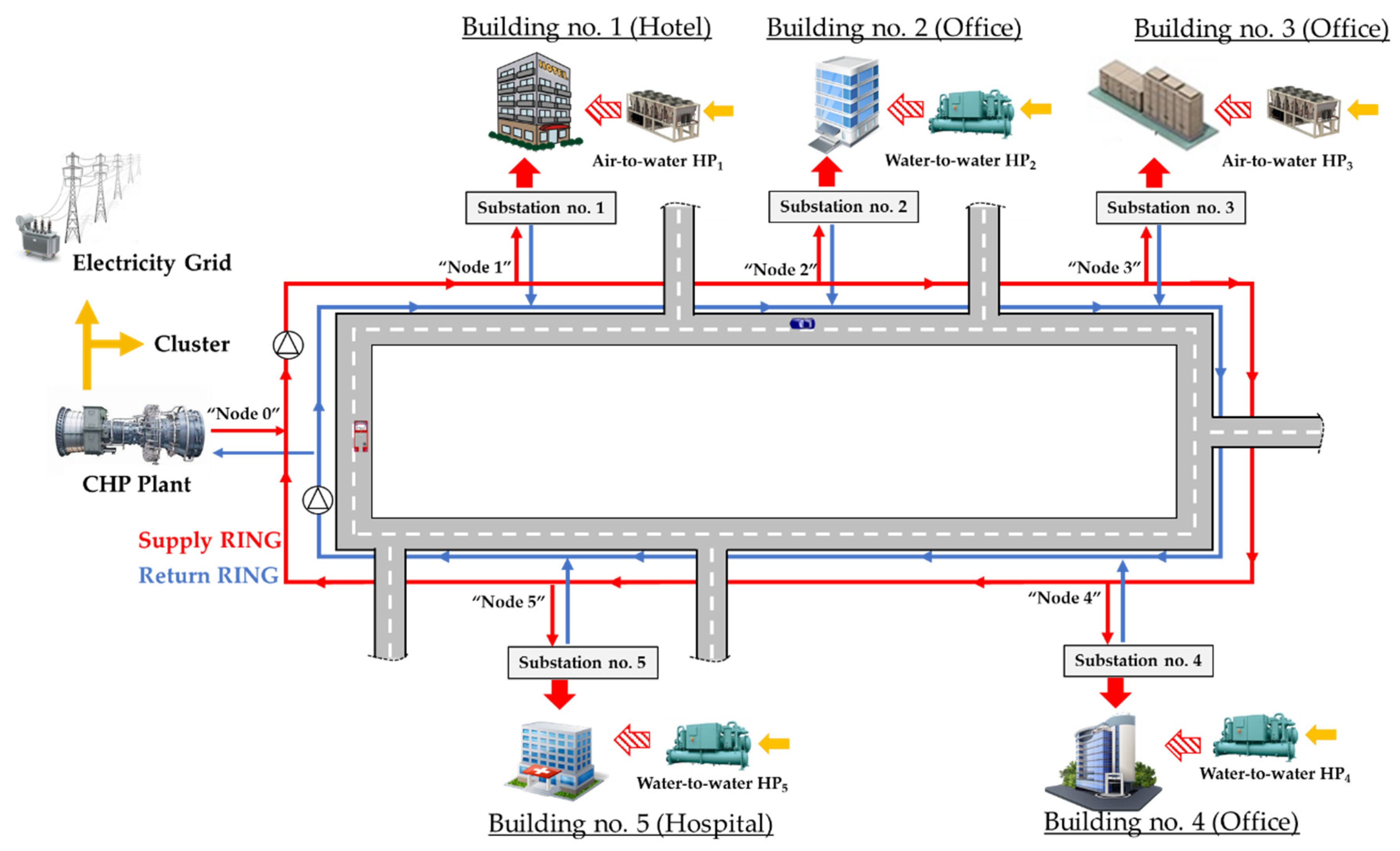
To show the capabilities of exergoeconomic cost accounting, a cluster of five buildings of the tertiary sectors was considered. A scheme is shown in Figure 4. The cluster was assumed to be located in the Mediterranean area, more specifically in Sicily (Italy). The following buildings were included: three offices, one hospital, and one hotel. Distances among nodes are presented in Table 1 (indicated by the letter “L”, respectively).

A CHP plant based on a GT as the prime mover was assumed to supply electricity and cover the thermal demands of the cluster. Moreover, natural gas (NG) was assumed to supply the prime mover. As shown in Figure 4, the position of the CHP plant is indicated by “Node 0”, and it was selected considering that Building no. 1 and Building no. 5 are large energy consumers. Finally, reversible HPs are installed at each consumer, not only to supply the uncovered part of thermal demands (for instance, in case of thermal demand under the minimum running capacity of the prime mover) but also for the sake of redundancy.

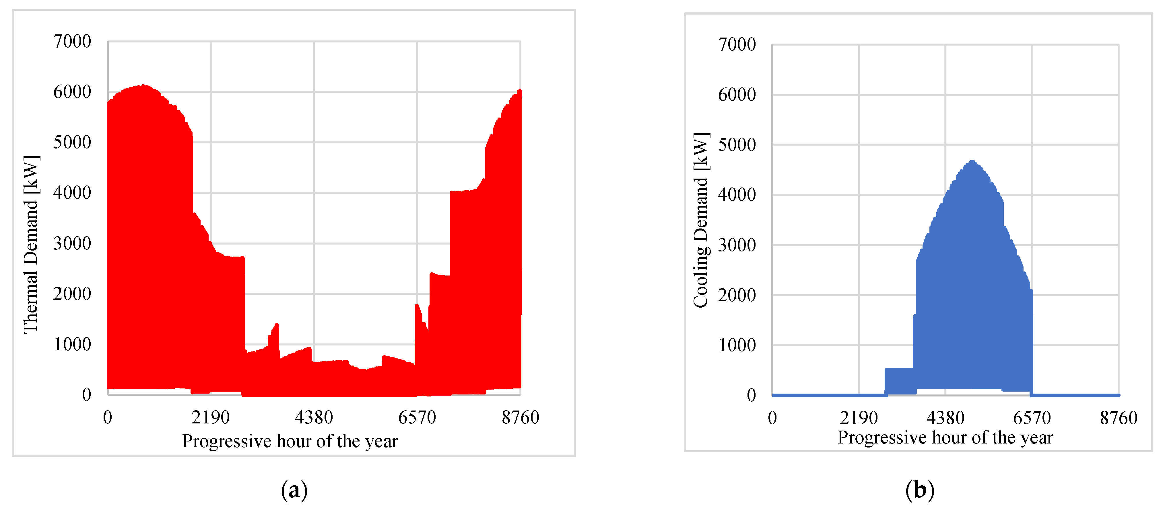
Aggregated hourly heating and cooling demands of the cluster are shown in Figure 5a,b respectively. Such profiles were obtained by summing up the hourly demand of each building, which were already published in a previous study by one of the authors [52].

Looking at Figure 5a,b, a peak of around 6.1 MW_th and 4.8 MW_c were observed for the thermal and cooling demand, respectively. A GT with a nominal electrical and thermal capacity equal to 4.7 MW_e and 7.0 MWth is assumed to be installed. This nominal capacity was selected considering a 7.3 MWth peak of the “aggregated thermal demand” (which was found by assuming the possibility to cover the overall cooling demand by using absorption chillers installed at each user substation with an average COP = 0.7 [53]).

In the reference scenario (indicated in the following as “Base Case”), the thermal grid was supplied by pressurized hot water at 85 °C and 12 bar (a typical operating temperature for thermal grids of the 3rd generation [4]), heated up using thermal energy recovered from the GT.

The nominal heating and cooling capacity of HPs (along with the COP and Energy Efficiency Ratio (EER) values) are shown in

Table 2. Main data of the thermal grid and HPs.

	Length		Number of Installed Units	HC 1	COP 1	CC 2	EER 2
	[m]			[kW]	[-]	[kW]	[-]
Branch 0–1	300	HP1 (Air-to-Water)	3	526	3.17	497	2.81
Branch 1–2	375	HP2 (Water-to-Water)	2	410	4.34	362	4.55
Branch 2–3	275	HP3 (Air-to-Water)	2	278	3.26	277	3.24
Branch 3–4	400	HP4 (Water-to-Water)	1	551	4.05	553	5.23
Branch 4–5	500	HP5 (Water-to-Water)	3	889	4.42	845	5.01
Branch 5–0	300

¹ Heating capacity refers to the following boundary conditions: variation of the water temperature in the condenser from 40 to 45 °C and outdoor air temperature equal to 7 °C. ² Cooling capacity refers to the following boundary conditions: variation of the water temperature in the evaporator from 7 to 12 °C, and outdoor air temperature equal to 35 °C (such boundary conditions are also used for the water-cooled chiller, with water entering the condenser equal to 30 °C).

. HPs were selected on the basis of the maximum cooling demands of each building, among those commercially available.

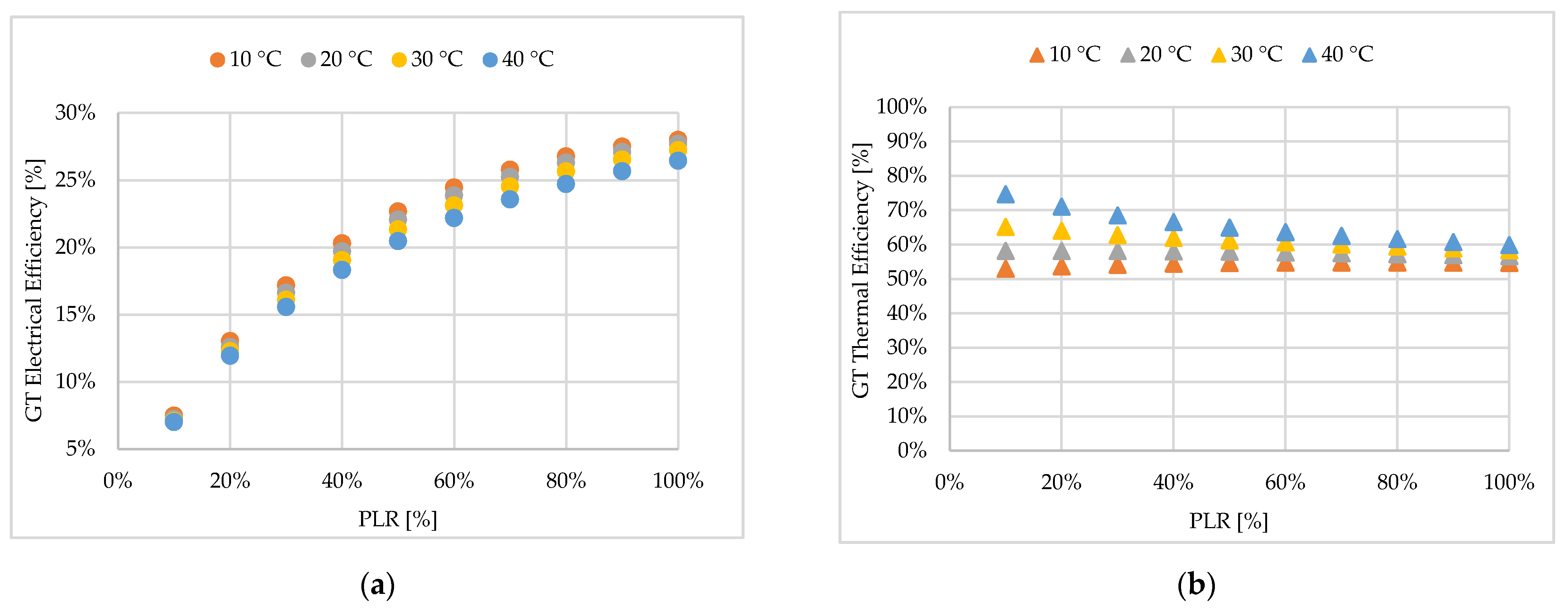
A typical CHP performance curve at full- and part-load operation was included in this study. The curves are shown in Figure 6. A decrease in the energy performance of the prime mover is observed when operating at part-load and the cut-off limit was assumed to be 10% of the nominal electrical power.

Description of the Simulated Scenarios, Assumptions and Limitations

The following two exemplificative scenarios were simulated and compared to the Base Case.

-

Scenario no. 1: It was assumed that due to the large surplus of electricity available from the local RES plant, a large water-to-water HP was installed aside from the CHP plant to convert the available surplus electricity into heat. The nominal thermal capacity of the HP was selected to cover 30% of the cluster heating demand. However, to allow for an efficient HP operation, the temperature of the grid was lowered from 85 °C down to 65 °C. Regarding COP of the large water-to-water HP, performance curves were developed from data available from the literature [55].

-

Scenario no. 2: It was assumed that the presence of two prosumers, more specifically Building no. 2 and no. 4, which during low or null thermal demand hours, supplied the excess heat produced by their HPs to the network. Furthermore, the heat available from the prosumers is produced via HPs using electricity from RES. The amount of thermal energy produced was quantified via Equation (16).

The internal tube diameter was selected limiting the value of the average pressure per unit length of the grid to 150–250 Pa/m. The nominal diameter of a pre-insulated steel pipe that satisfied this condition was 180 mm, with a linear heat transfer coefficient U_tube equal to 0.5 W/(m·°C).

Concerning the economic analysis, the investment costs of the main components were estimated by cost figures available in the following published papers [24,56,57] and are not repeated here for the sake of brevity. The CRF shown in Equation (11) was calculated assuming an interest rate equal to 7% and a 30-year plant life cycle. A CRF = 0.0806 was found.

It was assumed that the price of NG consumed by the CHP prime mover was equal to 27 c€/Nm³. Regarding the electricity available from local RES, it was assumed to be provided at an average price of 4.0 c€/kWh_el.

Both the physical and the exergoeconomic modeling presented in Section 2 were jointly solved using the Engineering Equation Solver (EES) [58]. It is worth noting that due to the intrinsic dynamic behavior of the network (thermal inertia, the finite velocity of water in tubes, etc.), the summation of the thermal demands of the buildings at a certain time might be different from the thermal power produced by the power plant. This hypothesis is the main assumption of this study. This fact could not be true in the case of large networks, for which the physical and exergoeconomic models of the network should be dynamically solved. Note that the possibility to solve dynamically exergoeconomic models of energy systems has been already addressed in literature by some of the authors [41,59]. In this paper, this aspect was not considered due to the low extension of the network.

4. Results and Discussion

Before showing the results of the exergoeconomic analysis of the investigated scenarios, it is worth discussing the ones obtained from the physical model. In Figure 7a,b pressure and temperature profiles are shown for the Base Case. In Figure 7a, the red curve is the pressure in SR. Conversely, the blue one is the pressure profile in the RR. The dotted lines are representative of the pressure setpoint of each pump. Note that:

-

a pressure drop equal to about 4.3 bar is observed in the SR during a full-load hour in winter when all the buildings are consuming heat from the grid. The profile among nodes is not smooth due to the different mass flow rate distribution in the branches of the network (see

Table 3. Main results of the physical model of the thermal grid in the Base Case.

	Mass Flowrate	Qloss		Mass Flowrate	Dth
	(kg/s)	(kW)		(kg/s)	(kW)
Branch 0–1	86.02	10.81	CHP	71.68	-
Branch 1–2	69.32	13.49	Bld. no. 1	16.70	1396
Branch 2–3	61.79	9.89	Bld. no. 2	7.53	628
Branch 3–4	49.71	14.37	Bld. no. 3	12.07	1005
Branch 4–5	44.66	17.95	Bld. no. 4	5.04	419
Branch 5–0	14.73	10.74	Bld. no. 5	29.93	2471

).

-

the temperature reduction in the supply ring network is estimated to be almost 0.5 °C, thanks to the U-value of the insulated tube. Temperature profiles are shown for the return ring as well, even though temperature variations are almost negligible (less than 0.2 °C). Looking at Table 3, simulation results indicated that the amount of thermal energy lost from the water circulating in the supply ring tube and transferred to the soil is around 78 kW_th.

4.1. Results for the Base Case

Results for the Base Case are presented in

Table 4. Exergoeconomic cost-accounting results for the Base Case.

	ki	kp*	kF*	cp	fz
	(kWex/kWex)	(kWex/kWex)	(kWex/kWex)	(c€/kWhex)	(%)
CHP	2.623	2.667	1.000	13.86	46.61
Pump HR	1.333	15.016	2.667	80.80	0.62
Pump CR	1.333	15.016	2.667	86.32	6.97
SubSt. no. 1	1.696	4.523	2.667	29.40	20.06
SubSt. no. 2	1.696	4.523	2.667	29.40	20.06
SubSt. no. 3	1.695	4.521	2.667	29.39	20.06
SubSt. no. 4	1.694	4.519	2.667	29.38	20.07
SubSt. no. 5	1.693	4.516	2.667	29.37	20.08

. The exergy consumption, the exergetic unit cost of product and fuel, and the exergoeconomic unit cost of products are shown. Note that:

-

an increase of the exergetic unit cost of the products k_p* from 2.667 up to 4.520 kW_ex/kW_ex is observed passing from the CHP plant to the buildings’ substation, due to the irreversibility cumulated along the process. Focusing on the substation building, the exergetic unit cost of the heat provided to the building (i.e., 4.520 kW_ex/kW_ex) is 1.69 times higher than the exergetic unit cost of the fuel (which is the exergy content of the pressurized hot water consumed from the grid which is equal to 2.667 kW_ex/kW_ex as shown in Table 4). Such an increase is testified by the exergy unit consumption of the substation, which is equal to or near 1.69 kW_ex/kW_ex, and it depends upon the irreversibility generated in the heat transfer in the substation building, between the hot water supplied by the grid and the water supplied to the hydronic circuit.

-

the exergy unit costs of the fuel consumed by the substation are approximately equal for all the users, meaning that the same irreversibility sources occurred along the productive process of the heat consumed, graphically depicted in Figure 2. Although such a result could be counterintuitive, as the different distance of the substation from the CHP plant leads to different pressure drops (and then irreversibility generation), the formulated model leads to an equal share of irreversibility generated due to pressure drop among users.

-

regarding the exergoeconomic unit cost of the heat supplied to the building, an average value of 29.4 c€/kWh_ex was found. This result is consequential not only to the equal share of irreversibility generated due to the pressure drop but also to the allocation criterion followed for the capital investment of the network, which distributes the investment cost proportionally to the exergy consumed by the users. In this respect, looking at the exergoeconomic factor f_z of the exergy product of the substation building, it could be noted that the capital investment accounted for nearly 20.1%.

Note that the high values of exergoeconomic unit cost shown in Table 4 are consequent to the low exergy content of the heat flow. Indeed, due to the low temperature of the supplied heat (85 °C), the exergy content is about 0.195 kWh_ex/kWh_th. If the unit cost of the heat found using the proposed method is then referred to the energy content, the value lowers down to 5.73 c€/kWh_th.

In Figure 8a,b, the exergetic and exergoeconomic unit costs of the heat are compared for a full-load hour on a weekday in the winter and a full-load hour on a weekend day in the same season. More specifically, for the full-load hour on the weekday, all users in the network are consuming heat, and an overall thermal demand equal to 5919 kW_th is observed. During the full-load hour on the weekend day, since offices are not open, the thermal demand is equal to 3743 kW_th. Due to reduced demand, the CHP mover will operate at part load (more specifically, with a PLR equal to 63%).

Looking at Figure 8a the exergetic unit cost of the CHP plant product increased from 2.667 to 2.826 kW_ex/kW_ex due to the part-load operation of the CHP prime mover (more specifically, a PLR equal to 60% was found). Indeed, as shown in Figure 6, when operated at PLR lower than 100%, the prime mover is characterized by a lower electrical energy performance (and then by a higher exergy unit consumption). Such an increase leads to a higher exergy unit cost of the heat produced in substations, which increases from 4.516 kW_ex/kW_ex up to 4.842 kW_ex/kW_ex.

The exergoeconomic unit cost of the consumed heat increases from 29.40 to 31.01 c€/kWh_ex. Although, as shown in Section 2, lower value thermal demand involves a reduction of the capital cost allocated to products, and increased CHP exergy unit consumption leads to higher exergoeconomic unit cost. Such a fact is also proved by the f_z values of the substations’ product (here not detailed shown for the sake of brevity), which decreased from 20.1% for full-load hours in the weekday to 19.03% in the part-load hours. The same consideration can be brought for full-load and part-load hours during a weekday.

It is trivial to say that no unit cost values are observed for offices in the weekend, as indicated by the absence of blue bars in Figure 8 for Substations no. 2–3 and 4, due to the null thermal demand.

4.2. Results for Scenario No. 1

Results for Scenario no. 1 are presented in

Table 5. Exergoeconomic cost-accounting results for Scenario no. 1.

	ki	kp*	cp	fz
	(kWex/kWex)	(kWex/kWex)	(c€/kWhex)	(%)
CHP	2.821	2.867	12.02	34.09
HP	2.020	2.237	33.776	96.93
Pump HR	1.333	23.568	110.812	0.83
SubSt. no. 1	1.244	3.332	28.972	20.36
SubSt. no. 2	1.244	3.332	28.973	20.36
SubSt. no. 3	1.243	3.330	28.956	20.37
SubSt. no. 4	1.243	3.330	28.958	20.37
SubSt. no. 5	1.242	3.327	28.933	20.38

. Note that:

-

the exergetic unit cost k_p* of the heat supplied to the buildings is equal to 3.330 kW_ex/kW_ex. Such a unit cost is 26.5% lower than the one obtained for the Base Case (shown in Table 4). Such a decrease is consequential to: (i) the insertion of water-to-water HP in the productive process, which leads to lower exergy destruction compared to CHP prime mover, as testified by the lower k_i of the HP in Table 5 compared to one of the CHP prime movers; and (ii) the lower exergy destruction occurring in the substation consequently to the lower operating temperature of the grid, as testified by the k_i of the substation which decreases from 1.7 to 1.24 kW_ex/kW_ex.

-

regarding the exergoeconomic unit cost of exergy of heat supplied to the building was found, its values are near −1.5% lower than the ones found in the Base Case (Table 4). The slight decrease is a combined effect of the investment cost required for the inclusion of the HP, and the lower amount of electricity produced by the CHP plant. However, since it was assumed to drive the HP using electricity produced by the RES plant, environmental benefits are achieved in terms of reduction of CO₂ emissions. If such benefits were accounted for by using an ad-hoc financial support mechanism, lower c_p values could be achieved.

-

looking at the exergoeconomic factor f_z, it could be noted that for HP, it is almost equal to 100%, since it is assumed that the electricity consumed is available at a very low price from renewable energy plants locally installed or from the electricity grid.

4.3. Results for Scenario No. 2

Before analyzing exergoeconomic analysis results for Scenario no. 2, it is worth discussing the results of the physical model.

In Figure 9, the pressure profile for the Base Case (dashed lines) and Scenario no. 2 (continuous lines) are shown. It is worth noting that pressure drops in the ring decrease when Building no. 2 and Building no. 4 act as producers, due to a different mass flow rate distribution in the network. The overall pressure drop in the supply ring reduces from 2.01 in the Base Case down to 1.40 bar in Scenario no. 2.

In

Table 6. Exergoeconomic cost-accounting results for Scenario no. 2.

	Base Case		Scenario No. 2
	kp*	cp	kp*	cp
	(kWex/kWex)	(c€/kWhex)	(kWex/kWex)	(c€/kWhex)
CHP	2.667	14.80	3.692	21.81
Pump HR	15.016	51.18	8.713	51.01
Pump CR	15.016	59.18	8.713	99.03
Subst. no. 1/Subst. no. 5	4.520	31.01	2.880	20.47

the exergy and exergoeconomic unit costs for Scenario no. 2 are shown along with the ones of the Base Case. The exergetic unit cost of the CHP plant product increased from 2.667 up to 3.692 kW_ex/kW_ex due to the part-load operation of the prime mover.

The exergetic unit cost k_p* of the heat supplied to the buildings decrease from 4.520 to 2.880 kW_ex/kW_ex. As observed for Scenario no. 1, such a decrease is achieved thanks to the heat generated via HP (which is characterized by lower k_i of the HP compared to one of the CHP prime movers) and the lower amount of exergy destroyed in substation (due to the reduced temperature of the supply ring).

Regarding the exergoeconomic unit cost of the heat supplied to the building, it was found that in Scenario no. 2, it is almost −33.9% lower than the value of the corresponding Base Case. Notably, no capital cost of prosumers’ HPs was allocated to the heat consumed by other users, since it was assumed that HPs were already paid back. The effects of this hypothesis will be discussed in the next section.

4.4. On the Use of the Proposed Model to Perform Sensitivity Analyses

To show the capability of the proposed method in supporting decisions during design and operation, two sensitivity analyses were performed. In particular:

-

The first analysis investigated the sensitivity of the exergoeconomic unit cost of the heat with the nominal diameter of the network for Scenario no. 1.

-

The second analysis considered for Scenario no. 2, the possibility to allocate the investment cost of prosumers’ HPs to other consumers of the grid.

In the first analysis, it was supposed to vary the diameter of the network from the reference value of 180 mm to the following values: 150 mm and 210 mm. When the diameter is decreased, a reduction of capital costs and an increase in pumping consumption are expected. Conversely, when the diameter is increased, an increase in the capital cost along with a decrease in pumping consumption is expected.

The results of this analysis are summarized in

Table 7. Results of the sensitivity analysis of exergoeconomic unit cost with tube diameter.

DN	Δp/L	cp	fz	kp*
(mm)	(Pa/m)	(c€/kWhex)	(%)	(kWex/kWex)
150	517.9	27.61	14.2	3.478
180	203.4	28.95	20.37	3.332
210	92.8	31.01	26.4	3.272

. Note that when the diameter is decreased, the exergoeconomic unit cost of the heat decreases, passing from 28.95 to 27.61 (−1.88%). Conversely, the exergy unit cost increases from 3.332 to 3.478 (+2.7%), due to the increase in pressure drops, as testified by values of Δp/L in Table 7. The joint use of the exergoeconomic unit cost and exergy unit cost suggests that although higher operating costs have to be sustained (due to increased pressure drop), the decrease of capital investment more than offset the extra operating cost.

Conversely, when the diameter is increased, the exergy unit cost of the heat consumed by the buildings decreased (due to lower pressure drop), but the increase of capital investment is not offset by the decrease of operating cost, as testified by comparing c_p and k_p* in Table 7.

Moreover, such a trend could be explained by observing the increasing values of f_z, which suggests an increasing influence of the capital investment on heat unit cost for a higher network diameter.

In the second analysis, it was found that the sensitivity of the exergoeconomic unit cost of the heat when the investment cost of prosumers’ HPs was also included. Following the criterion shown in Section 2 for the allocation of capital cost investment, it was assumed that capital costs related to the new HPs could be allocated according to the amount of product in the given hour. Moreover, the unit investment cost for HPs installed at Building no. 2 and no. 4 (whose capacities are shown in Table 2) was set equal to 350 €/kW.

In this case, results showed that if the capital cost of prosumers’ HPs is also allocated on the heat supplied to consumers, the exergoeconomic unit cost increased from 20.47 c€/kWh_ex (which was found in Section 4.3) to 24.54 c€/kWh_ex (+12.9%).

4.5. Further Potential Applications of the Proposed Model

Before ending, some notes on the further potential applications of the proposed model should be made. As previously pointed out, the proposed model should be solved jointly with a dynamical physical model of the network. This fact is of utmost importance considering also that energy storage equipment is increasingly applied in distributed energy systems to solve issues related to the mismatch between energy demand and production with high penetration of renewable energy sources. In this case, some refinements to the model presented in Section 2 are needed to account for the exergy stored or released by storage systems. Exergoeconomic analysis of energy systems which included energy storage systems has been performed in the literature as testified by the following published papers [46,60,61,62]. The proposed exergoeconomic model can be easily coupled with optimization methods for an efficient and cost-effective design of energy systems [63,64]. For instance, it could be possible to optimize the value of exergoeconomic unit costs considering synthesis, design, and operating variables, such as the CHP plant position, the installation of storage units, the operating temperature of the grid, and so on. Although environmental impacts, such as CO₂ emissions (or other impact categories), have not been considered in this analysis, the same procedure adopted for cost allocation can be followed to allocate emitted CO₂ on the exergy of the heat/cold distributed via DHC networks. The possibility to allocate environmental impacts on an exergy basis was already proposed in the literature and known as “Thermoecology”. The proposed model could be adopted for allocations of environmental impacts in DHC systems as well, and it could be very useful when different heat sources should be compared [65,66]. Finally, during the last few decades, “Thermoeconomic Diagnosis” has been proposed as a promising approach for the diagnosis of malfunctions occurring within an energy conversion system. The method aims at revealing, in a generic off-design operating condition due to “faulty” components within the system (e.g., fouling in heat exchangers, the efficiency of the pump, pipes restriction, insulation loss, etc., [67]), which are the faulty ones. In addition, it could quantify, in the case of multiple simultaneous faults, the effects on the overall system performance induced by each specific fault [68,69,70,71,72]. The proposed model could be assumed as a starting point to develop an exergoeconomic-based tool to perform the diagnosis of faults occurring in thermal grids.

5. Conclusions

In this paper, exergoeconomic cost accounting has been proposed as a method for cost allocation in DHC networks. To show the capabilities of this method, some operating scenarios were simulated and compared for a cluster of five buildings of the tertiary sector interconnected by a ring-shaped thermal grid. The analysis performed by the joint use of the exergy unit cost, exergoeconomic unit cost, and exergoeconomic factor allowed for a thorough comprehension of the effect of design and operating variables on heat unit cost. Starting from a Base Case where a centralized CHP plant was assumed to cover the thermal demand of the cluster, it was found that irreversibility occurring in the CHP plant and substations highly contributed to an increase in the exergetic unit cost of the heat produced. These results suggested that if the amount of irreversibility generated in the CHP prime mover and substations is reduced, the lower operating costs have to be sustained. Moreover, the exergoeconomic factor pointed out that capital investment may contribute to the heat unit cost by about 20%. When a centralized HP is installed to cover a fraction of the thermal demand, the analysis revealed that although less exergy is destroyed along the productive process of the heat, a slight decrease of exergoeconomic unit cost of the heat provided to consumers (near −1.5%) was obtained. Such a trend was consequential to the additional capital investment sustained for including the heat pump, and due to the lower amount of electricity produced by the CHP plant. Finally, if prosumers are operating, it was possible to quantify the unit cost could be lowered by about 33%.

The proposed model was revealed to be useful for the analysis of the exergoeconomic unit cost with the effect of changing key variables of the problem. To show these capabilities, two sensitivity analyses of the exergoeconomic unit cost of heat were performed. First, the effect of changes in the diameter of the ring was investigated, and the coordinated use of the exergy unit cost, exergoeconomic unit cost, and exergoeconomic factors revealed that variation of capital costs predominantly changes operating costs. Then, the possibility to allocate the investment cost of prosumers’ HP was considered and changes in the unit cost of heat could be quantified. In conclusion, the present study confirmed that Exergoeconomics could represent precious support in the analysis of thermal grids. Further prospects for improvement of the method exist, mainly lying in the possibility to develop optimization procedures and diagnostic tools.

References

1. Ürge-Vorsatz, D.; Cabeza, L.F.; Serrano, S.; Barreneche, C.; Petrichenko, K. Heating and Cooling Energy Trends and Drivers in Buildings. Renew. Sustain. Energy Rev. 2015, 41, 85–98. [Google Scholar] [CrossRef] [Green Version]
2. Economidou, M.; Todeschi, V.; Bertoldi, P.; D’Agostino, D.; Zangheri, P.; Castellazzi, L. Review of 50 years of EU Energy Efficiency Policies for Buildings. Energy Build. 2020, 225, 110322. [Google Scholar] [CrossRef]
3. Lund, H.; Werner, S.; Wiltshire, R.; Svendsen, S.; Thorsen, J.E.; Hvelplund, F.; Mathiesen, B.V. 4th Generation District Heating (4GDH): Integrating Smart Thermal Grids into Future Sustainable Energy Systems. Energy 2014, 68, 1–11. [Google Scholar] [CrossRef]
4. Werner, S. International Review of District Heating and Cooling. Energy 2017, 137, 617–631. [Google Scholar] [CrossRef]
5. Fahl, U.; Dobbins, A. Chapter 29—District Heating in Europe: Opportunities for Energy Savings, Business, and Jobs; Welsch, M., Pye, S., Keles, D., Faure-Schuyer, A., Dobbins, A., Shivakumar, A., Deane, P., Howells, M.B.T.-E.E.T., Eds.; Academic Press: Amsterdam, The Netherlands, 2017; pp. 249–259. ISBN 978-0-12-809806-6. [Google Scholar]
6. Tozlu, A.; Abusoglu, A.; Ozahi, E.; Anvari-Moghaddam, A. Municipal Solid Waste-Based District Heating and Electricity Production: A Case Study. J. Clean. Prod. 2021, 297, 126495. [Google Scholar] [CrossRef]
7. Aste, N.; Caputo, P.; del Pero, C.; Ferla, G.; Huerto-Cardenas, H.E.; Leonforte, F.; Miglioli, A. A Renewable Energy Scenario for a New Low Carbon Settlement in Northern Italy: Biomass District Heating Coupled with Heat Pump and Solar Photovoltaic System. Energy 2020, 206, 118091. [Google Scholar] [CrossRef]
8. Colmenar-Santos, A.; Rosales-Asensio, E.; Borge-Diez, D.; Blanes-Peiró, J.-J. District Heating and Cogeneration in the EU-28: Current Situation, Potential and Proposed Energy Strategy for Its Generalisation. Renew. Sustain. Energy Rev. 2016, 62, 621–639. [Google Scholar] [CrossRef]
9. Mathiesen, B.V.; Lund, H.; Connolly, D.; Wenzel, H.; Østergaard, P.A.; Möller, B.; Nielsen, S.; Ridjan, I.; Karnøe, P.; Sperling, K.; et al. Smart Energy Systems for Coherent 100% Renewable Energy and Transport Solutions. Appl. Energy 2015, 145, 139–154. [Google Scholar] [CrossRef]
10. Salpakari, J.; Mikkola, J.; Lund, P.D. Improved Flexibility with Large-Scale Variable Renewable Power in Cities through Optimal Demand Side Management and Power-to-Heat Conversion. Energy Convers. Manag. 2016, 126, 649–661. [Google Scholar] [CrossRef] [Green Version]
11. Gudmundsson, O.; Thorsen, J.E.; Brand, M. The Role of District Heating in Coupling of the Future Renewable Energy Sectors. Energy Procedia 2018, 149, 445–454. [Google Scholar] [CrossRef]
12. Buffa, S.; Cozzini, M.; D’Antoni, M.; Baratieri, M.; Fedrizzi, R. 5th Generation District Heating and Cooling Systems: A Review of Existing Cases in Europe. Renew. Sustain. Energy Rev. 2019, 104, 504–522. [Google Scholar] [CrossRef]
13. Sameti, M.; Haghighat, F. Optimization of 4th Generation Distributed District Heating System: Design and Planning of Combined Heat and Power. Renew. Energy 2019, 130, 371–387. [Google Scholar] [CrossRef]
14. Brange, L.; Englund, J.; Lauenburg, P. Prosumers in District Heating Networks—A Swedish Case Study. Appl. Energy 2016, 164, 492–500. [Google Scholar] [CrossRef]
15. von Rhein, J.; Henze, G.P.; Long, N.; Fu, Y. Development of a Topology Analysis Tool for Fifth-Generation District Heating and Cooling Networks. Energy Convers. Manag. 2019, 196, 705–716. [Google Scholar] [CrossRef]
16. Eremin, A.; Trubitsyn, K.; Kolesnikov, S.; Kudinov, I.; Tkachev, V. Computer Models of Hydraulic Systems of District Heating. MATEC Web Conf. 2018, 193, 02028. [Google Scholar] [CrossRef]
17. Bünning, F.; Wetter, M.; Fuchs, M.; Müller, D. Bidirectional Low Temperature District Energy Systems with Agent-Based Control: Performance Comparison and Operation Optimization. Appl. Energy 2018, 209, 502–515. [Google Scholar] [CrossRef] [Green Version]
18. Allegrini, J.; Orehounig, K.; Mavromatidis, G.; Ruesch, F.; Dorer, V.; Evins, R. A Review of Modelling Approaches and Tools for the Simulation of District-Scale Energy Systems. Renew. Sustain. Energy Rev. 2015, 52, 1391–1404. [Google Scholar] [CrossRef]
19. Neri, M.; Guelpa, E.; Verda, V. Design and Connection Optimization of a District Cooling Network: Mixed Integer Programming and Heuristic Approach. Appl. Energy 2022, 306, 117994. [Google Scholar] [CrossRef]
20. Wirtz, M.; Kivilip, L.; Remmen, P.; Müller, D. 5th Generation District Heating: A Novel Design Approach Based on Mathematical Optimization. Applied Energy 2020, 260, 114158. [Google Scholar] [CrossRef]
21. Fang, T.; Lahdelma, R. Genetic Optimization of Multi-Plant Heat Production in District Heating Networks. Applied Energy 2015, 159, 610–619. [Google Scholar] [CrossRef]
22. Gudmundsson, O.; Schmidt, R.-R.; Dyrelund, A.; Thorsen, J.E. Economic Comparison of 4GDH and 5GDH Systems—Using a Case Study. Energy 2022, 238, 121613. [Google Scholar] [CrossRef]
23. Sun, Q.; Li, H.; Wallin, F.; Zhang, Q. Marginal Costs for District Heating. Energy Procedia 2016, 104, 323–328. [Google Scholar] [CrossRef]
24. Alajmi, A.; Zedan, M. Energy, Cost, and Environmental Analysis of Individuals and District Cooling Systems for a New Residential City. Sustain. Cities Soc. 2020, 54, 101976. [Google Scholar] [CrossRef]
25. Tian, Z.; Perers, B.; Furbo, S.; Fan, J. Thermo-Economic Optimization of a Hybrid Solar District Heating Plant with Flat Plate Collectors and Parabolic Trough Collectors in Series. Energy Convers. Manag. 2018, 165, 92–101. [Google Scholar] [CrossRef] [Green Version]
26. Dorotić, H.; Pukšec, T.; Schneider, D.R.; Duić, N. Evaluation of District Heating with Regard to Individual Systems—Importance of Carbon and Cost Allocation in Cogeneration Units. Energy 2021, 221, 119905. [Google Scholar] [CrossRef]
27. Li, H.; Song, J.; Sun, Q.; Wallin, F.; Zhang, Q. A Dynamic Price Model Based on Levelized Cost for District Heating. Energy Ecol. Environ. 2019, 4, 15–25. [Google Scholar] [CrossRef] [Green Version]
28. Millar, M.-A.; Yu, Z.; Burnside, N.; Jones, G.; Elrick, B. Identification of Key Performance Indicators and Complimentary Load Profiles for 5th Generation District Energy Networks. Appl. Energy 2021, 291, 116672. [Google Scholar] [CrossRef]
29. Fahlén, E.; Ahlgren, E.O. Accounting for External Environmental Costs in a Study of a Swedish District-Heating System—An Assessment of Simplified Approaches. J. Clean. Prod. 2012, 27, 165–176. [Google Scholar] [CrossRef]
30. Erlach, B.; Serra, L.; Valero, A. Structural Theory as Standard for Thermoeconomics. Energy Convers. Manag. 1999, 40, 1627–1649. [Google Scholar] [CrossRef]
31. Cuadra, C.T. Symbolic Thermoeconomic Analysis of Energy Systems. In Exergy, Energy System Analysis and Optimization—Vol. II; Frangopoulos, C.A., Ed.; Encyclopedia of Life Support Systems (EOLSS): Paris, France, 2009. [Google Scholar]
32. Catrini, P.; Cipollina, A.; Micale, G.; Piacentino, A.; Tamburini, A. Exergy Analysis and Thermoeconomic Cost Accounting of a Combined Heat and Power Steam Cycle Integrated with a Multi Effect Distillation-Thermal Vapour Compression Desalination Plant. Energy Convers. Manag. 2017, 149, 950–965. [Google Scholar] [CrossRef]
33. Gaggioli, R.A.; Wepfer, W.J. Exergy Economics: I. Cost Accounting Applications. Energy 1980, 5, 823–837. [Google Scholar] [CrossRef]
34. Verda, V.; Caccin, M.; Kona, A. Thermoeconomic Cost Assessment in Future District Heating Networks. Energy 2016, 117, 485–491. [Google Scholar] [CrossRef]
35. Evans, R.B.; Tribus, M. Thermo-Economics of Saline Water Conversion. Ind. Eng. Chem. Process Des. Dev. 1965, 4, 195–206. [Google Scholar] [CrossRef]
36. Ozgener, L.; Hepbasli, A.; Dincer, I.; Rosen, M.A. Exergoeconomic Analysis of Geothermal District Heating Systems: A Case Study. Appl. Therm. Eng. 2007, 27, 1303–1310. [Google Scholar] [CrossRef]
37. Lozano, M.A.; Anastasia, A.; Serra, L.M.; Verda, V. Thermoeconomic Cost Analysis of Central Solar Heating Plants Combined with Seasonal Storage. In Proceedings of the ASME International Mechanical Engineering Congress and Exposition 2010, Vancouver, BC, Canada, 12–18 November 2010. [Google Scholar]
38. Van Erdeweghe, S.; van Bael, J.; D’haeseleer, W. Costing Methods for Combined Heat-and-Power Plants Fueled by Zero-Marginal Cost Energy Sources. Energy Convers. Manag. 2019, 187, 122–132. [Google Scholar] [CrossRef]
39. Oktay, Z.; Dincer, I. Exergoeconomic Analysis of the Gonen Geothermal District Heating System for Buildings. Energy Build. 2009, 41, 154–163. [Google Scholar] [CrossRef]
40. Tan, M.; Keçebaş, A. Thermodynamic and Economic Evaluations of a Geothermal District Heating System Using Advanced Exergy-Based Methods. Energy Convers. Manag. 2014, 77, 504–513. [Google Scholar] [CrossRef]
41. Meesenburg, W.; Ommen, T.; Elmegaard, B. Dynamic Exergoeconomic Analysis of a Heat Pump System Used for Ancillary Services in an Integrated Energy System. Energy 2018, 152, 154–165. [Google Scholar] [CrossRef] [Green Version]
42. Salehi, S.; Yari, M.; Rosen, M.A. Exergoeconomic Comparison of Solar-Assisted Absorption Heat Pumps, Solar Heaters and Gas Boiler Systems for District Heating in Sarein Town, Iran. Appl. Therm. Eng. 2019, 153, 409–425. [Google Scholar] [CrossRef]
43. Čož, T.D.; Kitanovski, A.; Poredoš, A. Exergoeconomic Optimization of a District Cooling Network. Energy 2017, 135, 342–351. [Google Scholar] [CrossRef]
44. Calise, F.; d’Accadia, M.D.; Macaluso, A.; Piacentino, A.; Vanoli, L. Exergetic and Exergoeconomic Analysis of a Novel Hybrid Solar–Geothermal Polygeneration System Producing Energy and Water. Energy Convers. Manag. 2016, 115, 200–220. [Google Scholar] [CrossRef]
45. Coss, S.; Guelpa, E.; Letournel, E.; Le-Corre, O.; Verda, V. Formulation of Exergy Cost Analysis to Graph-Based Thermal Network Models. Entropy 2017, 19, 109. [Google Scholar] [CrossRef]
46. Bagdanavicius, A.; Jenkins, N. Exergy and Exergoeconomic Analysis of a Compressed Air Energy Storage Combined with a District Energy System. Energy Convers. Manag. 2014, 77, 432–440. [Google Scholar] [CrossRef] [Green Version]
47. Torres, C.; Valero, A.; Rangel, V.; Zaleta, A. On the Cost Formation Process of the Residues. Energy 2008, 33, 144–152. [Google Scholar] [CrossRef]
48. Piacentino, A.; Cardona, F. On Thermoeconomics of Energy Systems at Variable Load Conditions: Integrated Optimization of Plant Design and Operation. Energy Convers. Manag. 2007, 48, 2341–2355. [Google Scholar] [CrossRef]
49. Lozano, M.A.; Valero, A. Theory of the Exergetic Cost. Energy 1993, 18, 939–960. [Google Scholar] [CrossRef]
50. Kotas, T.J. The Exergy Method of Thermal Plant Analysis; Butterworths: London, UK, 1985; Volume 20, ISBN 0894649418. [Google Scholar]
51. Bejan, A. Advanced Engineering Thermodynamics, 4th ed.; WILEY: New York, NY, USA, 2016. [Google Scholar]
52. Piacentino, A.; Barbaro, C. A Comprehensive Tool for Efficient Design and Operation of Polygeneration-Based Energy Μgrids Serving a Cluster of Buildings. Part II: Analysis of the Applicative Potential. Appl. Energy 2013, 111, 1222–1238. [Google Scholar] [CrossRef]
53. Piacentino, A.; Cardona, F. An Original Multi-Objective Criterion for the Design of Small-Scale Polygeneration Systems Based on Realistic Operating Conditions. Appl. Therm. Eng. 2008, 28, 2391–2404. [Google Scholar] [CrossRef]
54. Klein, S.A. TRNSYS 17: A Transient System Simulation Program; University of Wisconsin: Madison, WI, USA, 2010. [Google Scholar]
55. Schibuola, L.; Scarpa, M. Experimental Analysis of the Performances of a Surface Water Source Heat Pump. Energy Build. 2016, 113, 182–188. [Google Scholar] [CrossRef]
56. Pieper, H.; Ommen, T.; Buhler, F.; Paaske, B.L.; Elmegaard, B.; Markussen, W.B. Allocation of Investment Costs for Large-Scale Heat Pumps Supplying District Heating. Energy Procedia 2018, 147, 358–367. [Google Scholar] [CrossRef]
57. Beccali, M.; Ciulla, G.; di Pietra, B.; Galatioto, A.; Leone, G.; Piacentino, A. Assessing the Feasibility of Cogeneration Retrofit and District Heating/Cooling Networks in Small Italian Islands. Energy 2017, 141, 2572–2586. [Google Scholar] [CrossRef]
58. Klein, S.A. Engineering Equation Solver Software (EES); F-Chart Software: Middleton, WI, USA, 2013. [Google Scholar]
59. Picallo-Perez, A.; Catrini, P.; Piacentino, A.; Sala, J.-M. A Novel Thermoeconomic Analysis under Dynamic Operating Conditions for Space Heating and Cooling Systems. Energy 2019, 180, 819–837. [Google Scholar] [CrossRef]
60. Mosaffa, A.H.; Garousi Farshi, L. Exergoeconomic and Environmental Analyses of an Air Conditioning System Using Thermal Energy Storage. Appl. Energy 2016, 162, 515–526. [Google Scholar] [CrossRef]
61. Xi, Z.; Eshaghi, S.; Sardari, F. Energy, Exergy, and Exergoeconomic Analysis of a Polygeneration System Driven by Solar Energy with a Thermal Energy Storage Tank for Power, Heating, and Freshwater Production. J. Energy Storage 2021, 36, 102429. [Google Scholar] [CrossRef]
62. Godarzi, A.A.; Jalilian, M.; Samimi, J.; Jokar, A.; Vesaghi, M.A. Design of a PCM Storage System for a Solar Absorption Chiller Based on Exergoeconomic Analysis and Genetic Algorithm. Int. J. Refrig. 2013, 36, 88–101. [Google Scholar] [CrossRef]
63. Sayyaadi, H.; Saffari, A. Thermoeconomic Optimization of Multi Effect Distillation Desalination Systems. Appl. Energy 2010, 87, 1122–1133. [Google Scholar] [CrossRef]
64. Xiong, J.; Zhao, H.; Zhang, C.; Zheng, C.; Luh, P.B. Thermoeconomic Operation Optimization of a Coal-Fired Power Plant. Energy 2012, 42, 486–496. [Google Scholar] [CrossRef]
65. Stanek, W.; Szargut, J.; Kolenda, Z.; Czarnowska, L. Exergo-Ecological and Economic Evaluation of a Nuclear Power Plant within the Whole Life Cycle. Energy 2016, 117, 369–377. [Google Scholar] [CrossRef]
66. Szargut, J.; Ziębik, A.; Stanek, W. Depletion of the Non-Renewable Natural Exergy Resources as a Measure of the Ecological Cost. Energy Convers. Manag. 2002, 43, 1149–1163. [Google Scholar] [CrossRef]
67. Guelpa, E.; Verda, V. Automatic Fouling Detection in District Heating Substations: Methodology and Tests. Appl. Energy 2020, 258, 114059. [Google Scholar] [CrossRef]
68. Torres, C.; Valero, A.; Serra, L.; Royo, J. Structural Theory and Thermoeconomic Diagnosis: Part I. On Malfunction and Dysfunction Analysis. Energy Convers. Manag. 2002, 43, 1503–1518. [Google Scholar] [CrossRef]
69. Valero, A.; Lerch, F.; Serra, L.; Royo, J. Structural Theory and Thermoeconomic Diagnosis: Part II: Application to an Actual Power Plant. Energy Convers. Manag. 2002, 43, 1519–1535. [Google Scholar] [CrossRef]
70. Piacentino, A.; Talamo, M. Innovative Thermoeconomic Diagnosis of Multiple Faults in Air Conditioning Units: Methodological Improvements and Increased Reliability of Results. Int. J. Refrig. 2013, 36, 2343–2365. [Google Scholar] [CrossRef]
71. Picallo-Perez, A.; Sala-Lizarraga, J.M.; Escudero-Revilla, C. A Comparative Analysis of Two Thermoeconomic Diagnosis Methodologies in a Building Heating and DHW Facility. Energy Build. 2017, 146, 160–171. [Google Scholar] [CrossRef]
72. Valero, A.; Correas, L.; Zaleta, A.; Lazzaretto, A.; Verda, V.; Reini, M.; Rangel, V. On the Thermoeconomic Approach to the Diagnosis of Energy System Malfunctions: Part 2. Malfunction Definitions and Assessment. Energy 2004, 29, 1889–1907. [Google Scholar] [CrossRef]
Figure 1. Scheme of the generic cluster of buildings served by the ring-shaped thermal network.
Sustainability 14 04004 g001
Figure 2. Productive structure of a ring-shaped thermal grid with a centralized heat producer.
Sustainability 14 04004 g002
Figure 3. Productive structure of a ring network with the presence of the prosumers.
Sustainability 14 04004 g003
Figure 4. Scheme of the cluster of buildings served by the thermal grid.
Sustainability 14 04004 g004
Figure 5. Energy demands of the cluster: (a) thermal demand (space heating and domestic hot water) and (b) cooling demand.
Sustainability 14 04004 g005
Figure 6. GT typical efficiency curves: (a) electrical and (b) thermal efficiency based on data available in [54], for five environmental temperature values (TOD).
Sustainability 14 04004 g006
Figure 7. Results of the physical model for the Base Case: (a) pressure profiles in the supply and return network; (b) temperature profile in the supply network.
Sustainability 14 04004 g007
Figure 8. Exergetic and exergoeconomic unit cost comparison for a full-load hour in: (a) a typical weekday in winter and (b) a typical weekend day.
Sustainability 14 04004 g008
Figure 9. Pressure profile in the network for Base Case (dashed lines) and Scenario no. 2 (continuous line).
Sustainability 14 04004 g009