
Adaptive DMA Design and Operation under Multiscenarios in Water Distribution Networks


Abstract
:1. Introduction
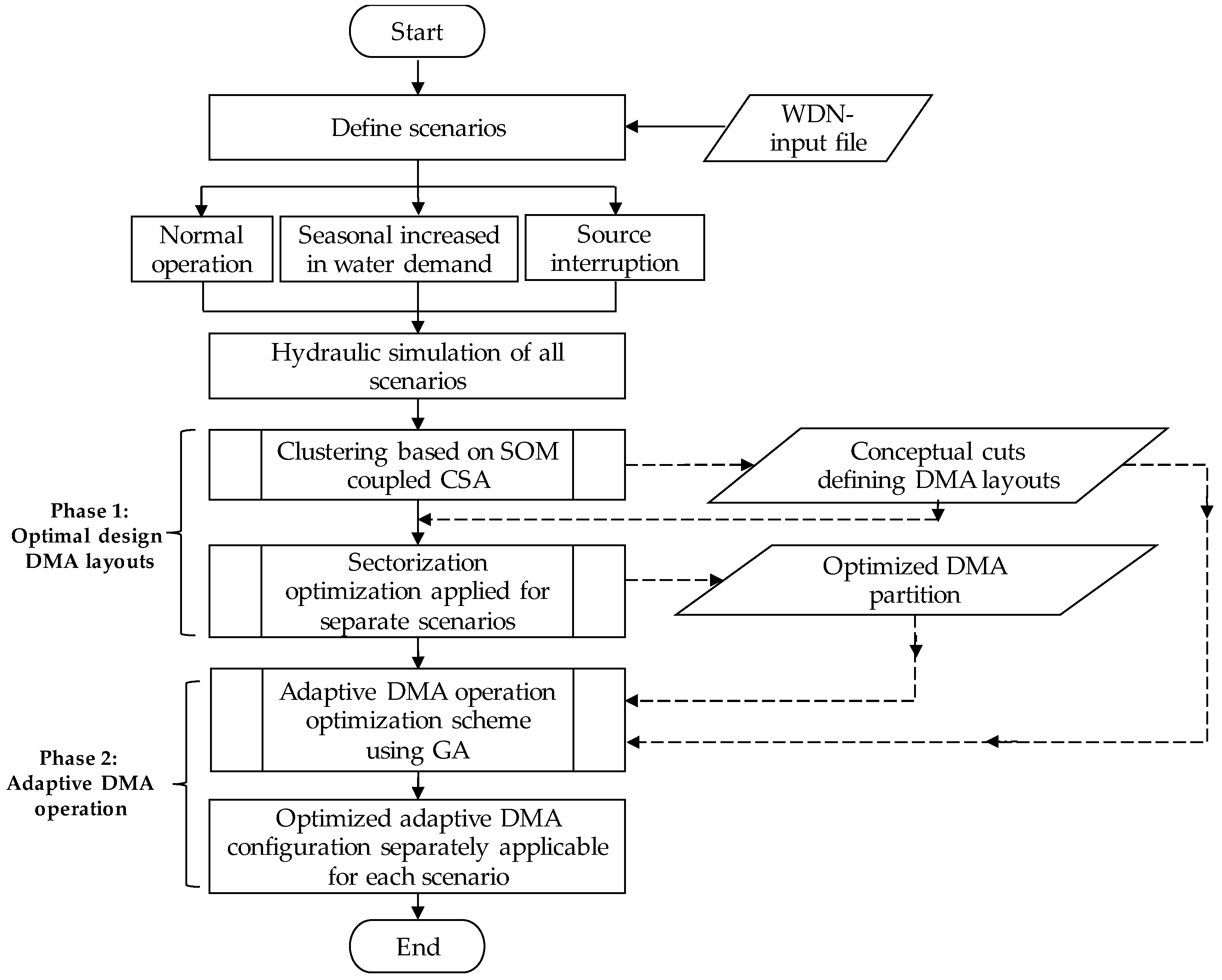
2. Methodology
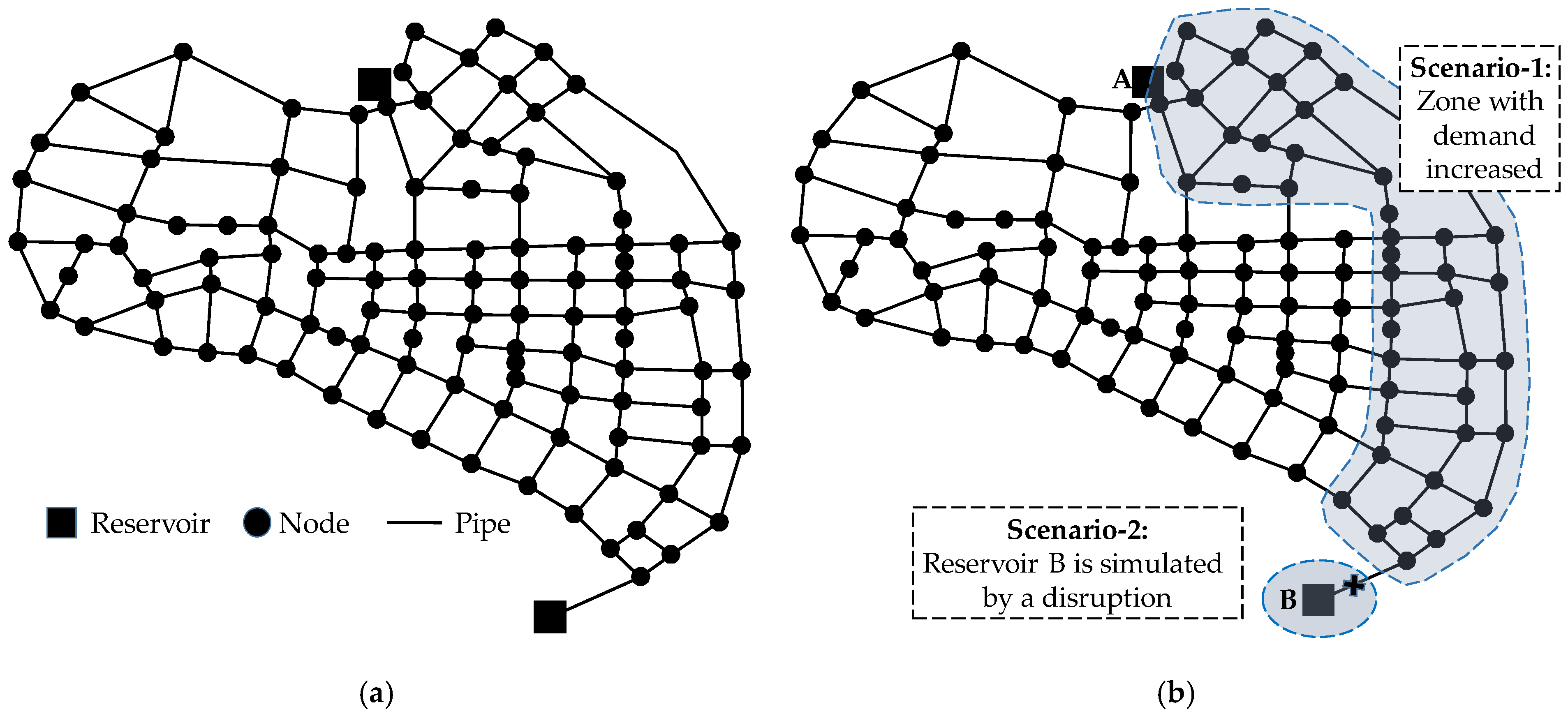
2.1. Scenario Creation
2.2. Water Network Partitioning
2.2.1. Clustering Phase
- The construction of the adjacency matrix (A) of an undirected network representing the connectivity of nodes i and node j, such that Aij = 1 if they are connected, otherwise Aij = 0.
- The topology similarity matrix (TS) represents the degree of node proximity in the network, i.e., the nodes in a pair are similar if they share several neighbors.
- The hydraulic similarity matrix (HS) was developed to quantify the correlation of pressure (p) and elevation (e) between a pair of connected nodes i and j in a WDN.
2.2.2. Sectorization Phase
2.3. Adaptive DMAs Design and Operation
- The deviation of the PU index between the adaptive DMAs and scenario-specific optimal DMAs is the smallest and applicable for multiple scenarios.
- The mean absolute percentage error (MAPE) of the nodal pressure between the adaptive DMAs and scenario-specific optimal DMAs is the lowest and applicable for multiple scenarios.
- Pressure uniformity deviation index, f1:
- Mean absolute percentage error (MAPE) of nodal pressure, f2:
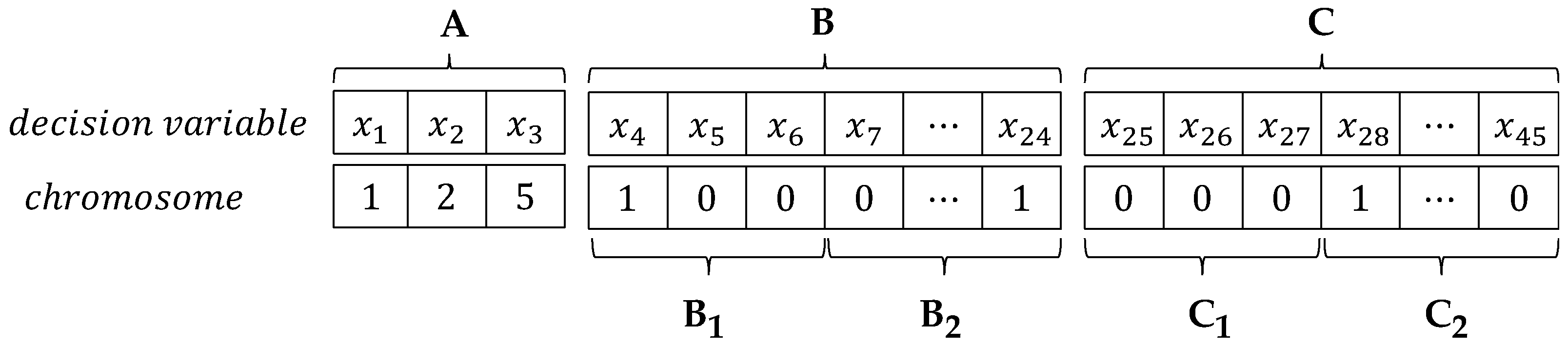
- , and denote the optimal set-cut pipes (i.e., boundary pipes) in the optimal DMA layouts of the base scenario, S1 and S2, respectively. Note that the base design with is given and fixed. Specifically, the sets of flow meters , gate valves , and their locations were settled.
- The set-cut pipes for all scenarios were uniquely defined as the union of the optimal set-cut pipes under various scenarios, expressed as
- The decision space for the control valve settings {SPcvs} (i.e., opened or closed) represents the union of a set of additional valves {SPadd.gv}, and a set of valves readily existed in the base design, expressed as
2.4. Adaptive DMA Layouts Assessment
3. Case Study and Application Results
3.1. Study Network
3.2. Optimal DMA Designs for Individual Scenarios
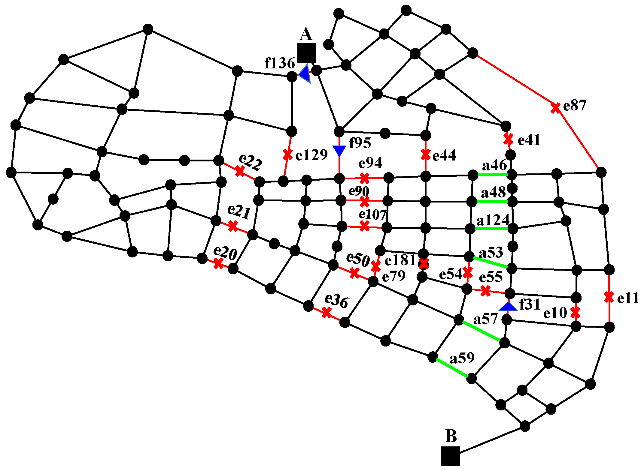
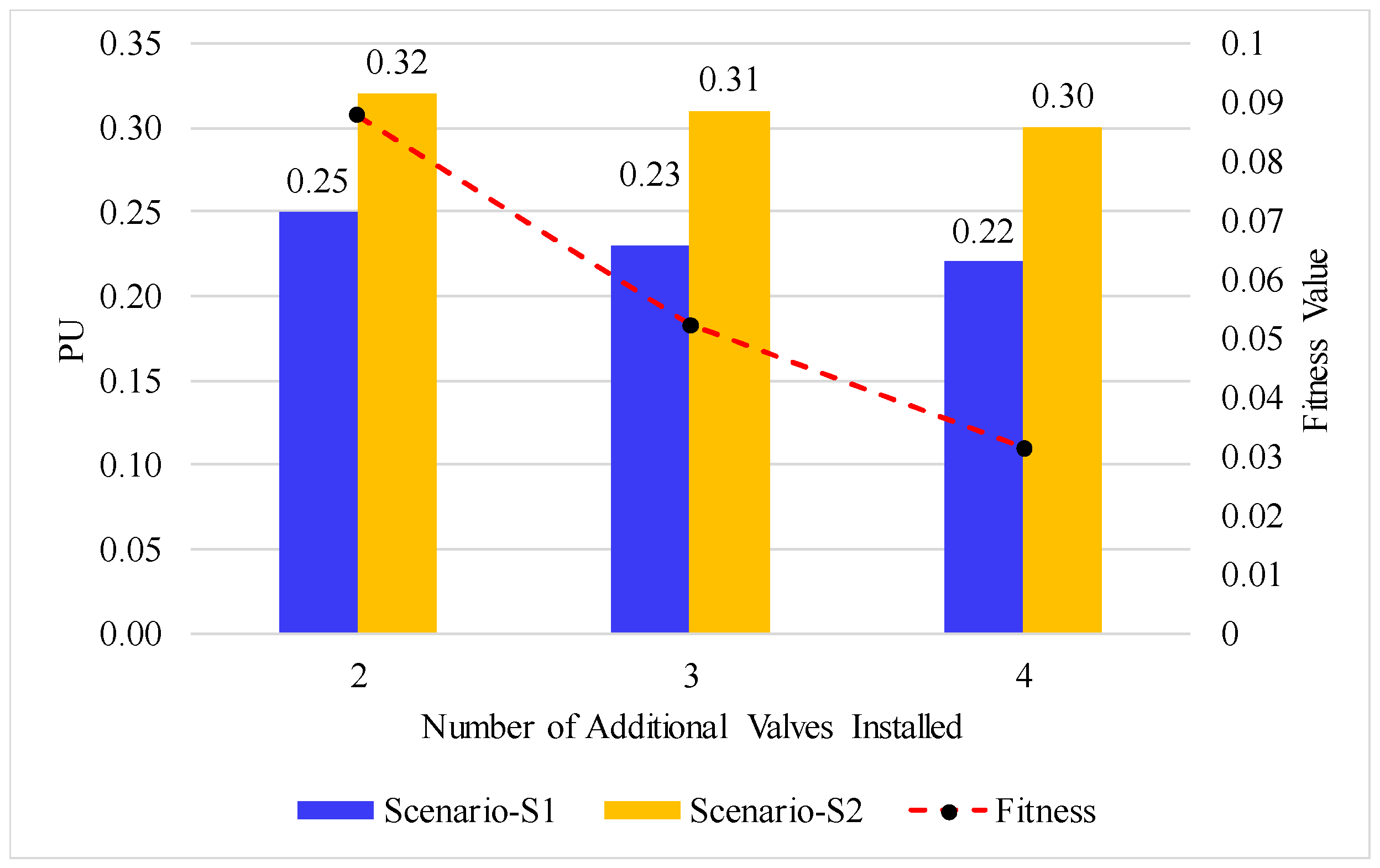
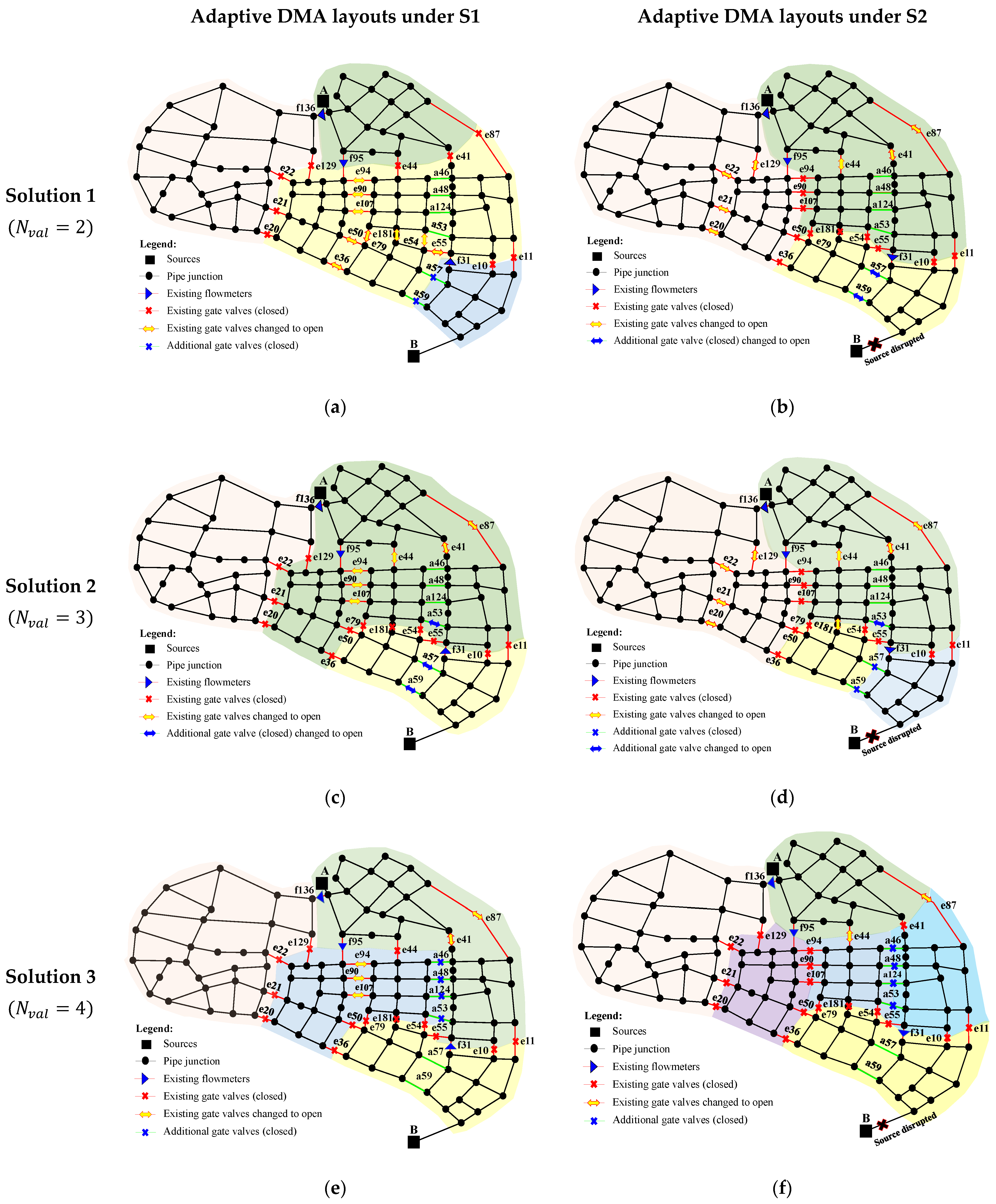
3.3. Adaptive DMAs with Additional Valve Installation
3.4. Adaptive DMA Operation under Abnormal Scenarios
4. Discussion
5. Conclusions
- The optimal DMA layouts for various plausible operational scenarios were created based on the minimization of the PU index and considered as a reference in the transformation stage for the adaptive DMA layouts applicable for individual scenarios.
- By providing a priori number and the location of the additional and existing valves that required control (e.g., closed or open), distinct adaptive DMA layouts could be obtained, separately applied in specific scenarios.
- The higher the number of additional valves installed, the better the hydraulic performance of adaptive DMAs obtained (e.g., pressure indices, PU, WLR, RMSE of pressure) to mimic the behavior of the optimal DMA layouts for specific scenarios.
Author Contributions
Funding
Institutional Review Board Statement
Informed Consent Statement
Data Availability Statement
Conflicts of Interest
References
- Gleick, P.H. The human right to water. Water Policy 1998, 1, 487–503. [Google Scholar] [CrossRef]
- United Nations. Transforming Our World: The 2020 Agenda for Sustainable Development; United Nations General Assembly: New York, NY, USA, 2015. [Google Scholar]
- Christodoulou, S.; Fragiadakis, M.; Agathokleous, A.; Xanthos, S. Urban Water Distribution Networks: Assessing Systems Vulnerabilities, Failures, and Risks; Butterworth-Heinemann: Oxford, UK, 2017. [Google Scholar]
- Taormina, R.; Galelli, S.; Tippenhauer, N.O.; Salomons, E.; Ostfeld, A.; Eliades, D.G.; Aghashahi, M.; Sundararajan, R.; Pourahmadi, M.; Banks, M.K.; et al. Battle of the attack detection algorithms: Disclosing cyber attacks on water distribution networks. J. Water Resour. Plan. Manag. 2018, 144, 04018048. [Google Scholar] [CrossRef] [Green Version]
- Kang, D.; Lansey, K. Multiperiod planning of water supply infrastructure based on scenario analysis. J. Water Resour. Plan. Manag. 2014, 140, 40–54. [Google Scholar] [CrossRef]
- Zechman Berglund, E.; Thelemaque, N.; Spearing, L.; Faust, K.M.; Kaminsky, J.; Sela, L.; Goharian, E.; Abokifa, A.; Lee, J.; Keck, J.; et al. Water and wastewater systems and utilities: Challenges and opportunities during the COVID-19 Pandemic. J. Water Resour. Plan. Manag. 2021, 147, 02521001. [Google Scholar] [CrossRef]
- Perelman, L.; Ostfeld, A. Topological clustering for water distribution systems analysis. Environ. Mod. Softw. 2011, 26, 969–972. [Google Scholar] [CrossRef]
- Malcolm, F. Sanitation water, water supply, sanitation collaborative council, and World Health Organization. In Leakage Management and Control: A Best Practice Training Manual; No. WHO/SDE/WSH/01.1; World Health Organization: Geneva, Switzerland, 2001. [Google Scholar]
- Walski, T.M.; Chase, D.V.; Savic, D.A.; Grayman, W.; Beckwith, S.; Koelle, E. Advanced water distribution modeling and management. In Civil and Environmental Engineering and Engineering Mechanics Faculty Publications; Haestad Press: Waterbury, CT, USA, 2003; Volume 18. [Google Scholar]
- Gomes, R.; Sá Marques, A.; Sousa, J. Estimation of the benefits yielded by pressure management in water distribution systems. Urban Water J. 2011, 8, 65–77. [Google Scholar] [CrossRef]
- Lifshitz, R.; Ostfeld, A. Clustering for analysis of water distribution systems. J. Water Resour. Plan. Manag. 2018, 144, 04018016. [Google Scholar] [CrossRef]
- Di Nardo, A.; Di Natale, M.; Guida, M.; Musmarra, D. Water network protection from intentional contamination by sectorization. Water Resour. Manag. 2013, 27, 1837–1850. [Google Scholar] [CrossRef]
- Ciaponi, C.; Creaco, E.; di Nardo, A.; di Natale, M.; Giudicianni, C.; Musmarra, D.; Santonastaso, G.F. Reducing impacts of contamination in water distribution networks: A combined strategy based on network partitioning and installation of water quality sensors. Water 2019, 11, 1315. [Google Scholar] [CrossRef] [Green Version]
- Giudicianni, C.; Herrera, M.; di Nardo, A.; Carravetta, A.; Ramos, H.M.; Adeyeye, K. Zero-net energy management for the monitoring and control of dynamically-partitioned smart water systems. J. Clean. Prod. 2020, 252, 119745. [Google Scholar] [CrossRef]
- Saldarriaga, J.; Bohorquez, J.; Celeita, D.; Vega, L.; Paez, D.; Savic, D.; Dandy, G.; Filion, Y.; Grayman, W.; Kapelan, Z. Battle of the water networks district metered areas. J. Water Resour. Plan. Manag. 2019, 145, 04019002. [Google Scholar] [CrossRef]
- Di Nardo, A.; Di Natale, M.; Santonastaso, G.F.; Venticinque, S. An automated tool for smart water network partitioning. Water Resour. Manag. 2013, 27, 4493–4508. [Google Scholar] [CrossRef]
- Bianchotti, J.D.; Denardi, M.; Castro-Gama, M.; Puccini, G.D. Sectorization for water distribution systems with multiple sources: A Performance Indices Comparison. Water 2021, 13, 131. [Google Scholar] [CrossRef]
- Di Nardo, A.; Di Natale, M.; Santonastaso, G.F.; Tzatchkov, V.G.; Alcocer-Yamanaka, V.H. Water network sectorization based on graph theory and energy performance indices. J. Water Resour. Plan. Manag. 2014, 140, 620–629. [Google Scholar] [CrossRef]
- Liu, J.; Han, R. Spectral clustering and multicriteria decision for design of district metered area. J. Water Resour. Plan. Manag. 2018, 144, 04018013. [Google Scholar] [CrossRef]
- Bui, X.K.; Marlim, M.S.; Kang, D. Optimal design of district metered areas in a water distribution network using coupled self-organizing map and community structure algorithm. Water 2021, 13, 836. [Google Scholar] [CrossRef]
- Zhang, K.; Yan, H.; Zeng, H.; Xin, K.; Tao, T. A practical multi-objective optimization sectorization method for water distribution network. Sci. Total Environ. 2019, 656, 1401–1412. [Google Scholar] [CrossRef]
- Vasilic, Ž.; Stanic, M.; Kapelan, Z.; Prodanovic, D.; Babic, B. Uniformity and heuristics-based DeNSE method for sectorization of water distribution networks. J. Water Resour. Plan. Manag. 2020, 146, 04019079. [Google Scholar] [CrossRef] [Green Version]
- Brentan, B.M.; Campbell, E.; Meirelles, G.L.; Luvizotto, E., Jr.; Izquierdo, J. Social network community detection for DMA creation: Criteria analysis through multilevel optimization. Math. Prob. Eng. 2017, 13, 1–12. [Google Scholar] [CrossRef]
- Diao, K.; Zhou, Y.; Rauch, W. Automated creation of district metered area boundaries in water distribution systems. J. Water Resour. Plan. Manag. 2013, 139, 184–190. [Google Scholar] [CrossRef]
- Di Nardo, A.; Giudicianni, C.; Greco, R.; Herrera, M.; Santonastaso, G. Applications of graph spectral techniques to water distribution network management. Water 2018, 10, 45. [Google Scholar] [CrossRef] [Green Version]
- Alvisi, S. A new procedure for optimal design of district metered areas based on the multilevel balancing and refinement algorithm. Water Resour. Manag. 2015, 29, 4397–4409. [Google Scholar] [CrossRef]
- Herrera, M.; Izquierdo, J.; Pérez-García, R.; Montalvo, I. Multi-agent adaptive boosting on semi-supervised water supply clusters. Adv. Eng. Softw. 2012, 50, 131–136. [Google Scholar] [CrossRef]
- Gomes, R.; Sá Marques, A.; Sousa, J. Identification of the optimal entry points at District Metered Areas and implementation of pressure management. Urban Water J. 2012, 9, 365–384. [Google Scholar] [CrossRef]
- Di Nardo, A.; Di Natale, M. A heuristic design support methodology based on graph theory for district metering of water supply networks. Eng. Optim. 2011, 43, 193–211. [Google Scholar] [CrossRef]
- Grayman, W.M.; Murray, R.; Savic, D.A. Effects of redesign of water systems for security and water quality factors. In Proceedings of the World Environmental and Water Resources Congress, Kansas City, MI, USA, 17–21 May 2009; pp. 1–11. [Google Scholar] [CrossRef]
- Laucelli, D.B.; Simone, A.; Berardi, L.; Giustolisi, O. Optimal design of district metering areas for the reduction of leakages. J. Water Resour. Plan. Manag. 2017, 143, 04017017. [Google Scholar] [CrossRef]
- Bui, X.K.; Marlim, M.S.; Kang, D. Water network partitioning into district metered areas: A state-of-the-art review. Water 2020, 12, 1002. [Google Scholar] [CrossRef] [Green Version]
- Mu, T.; Lu, Y.; Tan, H.; Zhang, H.; Zheng, C. Random walks partitioning and network reliability assessing in water distribution system. Water Resour. Manag. 2021, 35, 2325–2341. [Google Scholar] [CrossRef]
- Palleti, V.R.; Kurian, V.; Narasimhan, S.; Rengaswamy, R. Actuator network design to mitigate contamination effects in water distribution networks. Comput. Chem. Eng. 2018, 108, 194–205. [Google Scholar] [CrossRef]
- Creaco, E.; Haidar, H. Multiobjective optimization of control valve installation and DMA creation for reducing leakage in water distribution networks. J. Water Resour. Plan. Manag. 2019, 145, 04019046. [Google Scholar] [CrossRef]
- Zhang, T.; Yao, H.; Chu, S.; Yu, T.; Shao, Y. Optimized DMA partition to reduce background leakage rate in water distribution networks. J. Water Resour. Plan. Manag. 2021, 147, 04021071. [Google Scholar] [CrossRef]
- Rahmani, F.; Muhammed, K.; Behzadian, K.; Farmani, R. Optimal operation of water distribution systems using a graph theory–based configuration of district metered areas. J. Water Resour. Plan. Manag. 2018, 144, 04018042. [Google Scholar] [CrossRef]
- Brentan, B.M.; Carpitella, S.; Izquierdo, J.; Luvizotto, E.; Meirelles, G. District metered area design through multicriteria and multiobjective optimization. Math. Methods Appl. Sci. 2021, 45, 3254–3271. [Google Scholar] [CrossRef]
- Zeidan, M.; Li, P.; Ostfeld, A. DMA segmentation and multiobjective optimization for trading off water age, excess pressure, and pump operational cost in water distribution systems. J. Water Resour. Plan. Manag. 2021, 147, 04021006. [Google Scholar] [CrossRef]
- Wright, R.; Stoianov, I.; Parpas, P.; Henderson, K.; King, J. Adaptive water distribution networks with dynamically reconfigurable topology. J. Hydroinform. 2014, 16, 1280–1301. [Google Scholar] [CrossRef]
- Wright, R.; Abraham, E.; Parpas, P.; Stoianov, I. Control of water distribution networks with dynamic DMA topology using strictly feasible sequential convex programming: Water Distribution Networks with Dynamic Topology. Water Resour. Res. 2015, 51, 9925–9941. [Google Scholar] [CrossRef] [Green Version]
- Scarpa, F.; Lobba, A.; Becciu, G. Elementary DMA design of looped water distribution networks with multiple sources. J. Water Resour. Plan. Manag. 2016, 142, 04016011. [Google Scholar] [CrossRef] [Green Version]
- Giudicianni, C.; Herrera, M.; di Nardo, A.; Adeyeye, K. Automatic multiscale approach for water networks partitioning into dynamic district metered areas. Water Resour. Manag. 2020, 34, 835–848. [Google Scholar] [CrossRef] [Green Version]
- Kohonen, T. Self-organized formation of topologically correct feature maps. Biol. Cyber. 1982, 43, 59–69. [Google Scholar] [CrossRef]
- Clauset, A.; Newman, M.E.J.; Moore, C. Finding community structure in very large networks. Phys. Rev. E 2004, 70, 066111. [Google Scholar] [CrossRef] [Green Version]
- Wu, Z.Y.; Walski, T. Pressure dependent hydraulic modelling for water distribution systems under abnormal conditions. In Proceedings of the IWA World Water Congress and Exhibition, Beijing, China, 10–14 September 2006. [Google Scholar]
- Sivakumar, P.; Prasad, R.K. Simulation of water distribution network under pressure-deficient condition. Water Resour. Manag. 2014, 28, 3271–3290. [Google Scholar] [CrossRef]
- Newman, M.E.J. Fast algorithm for detecting community structure in networks. Phys. Rev. E 2004, 69, 066133. [Google Scholar] [CrossRef] [Green Version]
- Alhimiary, H.A.A.; Alsuhaily, R.H.S. Minimizing leakage rates in water distribution networks through optimal valves settings. In Proceedings of the World Environmental and Water Resources Congress, Tampa, FL, USA, 15–19 May 2007. [Google Scholar] [CrossRef]
- Ferrari, G.; Savic, D. Economic performance of DMAs in water distribution systems. Procedia Eng. 2015, 119, 189–195. [Google Scholar] [CrossRef] [Green Version]
- Giustolisi, O.; Savic, D.; Kapelan, Z. Pressure-driven demand and leakage simulation for water distribution networks. J. Hydraul. Eng. 2008, 134, 626–635. [Google Scholar] [CrossRef] [Green Version]
- Zheng, F.; Simpson, A.R.; Zecchin, A.C. A combined NLP-differential evolution algorithm approach for the optimization of looped water distribution systems. Water Resour. Res. 2011, 47, W08531. [Google Scholar] [CrossRef] [Green Version]
- Todini, E. Looped water distribution networks design using a resilience index based heuristic approach. Urban Water 2000, 2, 115–122. [Google Scholar] [CrossRef]
- Spearing, L.A.; Thelemaque, N.; Kaminsky, J.A.; Katz, L.E.; Kinney, K.A.; Kirisits, M.J.; Sela, L.; Faust, K.M. Implications of social distancing policies on drinking water infrastructure: An overview of the challenges to and responses of US Utilities during the COVID-19 pandemic. ACS ES&T Water 2020, 1, 888–899. [Google Scholar] [CrossRef]
- Kalbusch, A.; Henning, E.; Brikalski, M.P.; de Luca, F.V.; Konrath, A.C. Impact of coronavirus (COVID-19) spread-prevention actions on urban water consumption. Resour. Conserv. Recycl. 2020, 163, 105098. [Google Scholar] [CrossRef]
- Alvisi, S.; Franchini, M.; Luciani, C.; Marzola, I.; Mazzoni, F. Effects of the COVID-19 Lockdown on Water Consumptions: Northern Italy Case Study. J. Water Resour. Plan. Manag. 2021, 147, 05021021. [Google Scholar] [CrossRef]
- Jeong, G.; Kang, D.; Kim, K. Analysis on drinking water use change by COVID-19: A case study of residential area in S-city, South Korea. J. Korea Water Resour. Assoc. 2022, 55, 11–21. [Google Scholar] [CrossRef]
- Girón-Navarro, R.; Linares-Hernández, I.; Castillo-Suárez, L.A. The impact of coronavirus SARS-CoV-2 (COVID-19) in water: Potential risks. Environ. Sci. Pollut. Res. 2021, 28, 52651–52674. [Google Scholar] [CrossRef] [PubMed]
- Sahoo, P. The Adverse Effects of Estrogenic Pill Driven After Flexible Fertility on Environment in COVID-19 Situation. Eng. Sci. 2021, 14, 109–113. [Google Scholar] [CrossRef]


| Scenarios | No. of DMAs | Nbp | Nfm | Ngv | PU | RI | Pressure (m) | ||
|---|---|---|---|---|---|---|---|---|---|
| Hmax | Hmin | Hmean | |||||||
| Unpartitioned | – | – | – | 0.54 | 0.83 | 38.42 | 36.07 | 36.58 | |
| Base Scenario | 2 | 8 | 1 | 7 | 0.53 | 0.81 | 38.12 | 36.03 | 36.52 |
| 3 | 13 | 2 | 11 | 0.49 | 0.79 | 37.83 | 35.01 | 36.50 | |
| 4 | 20 | 3 | 17 | 0.48 | 0.77 | 37.75 | 34.60 | 36.00 | |
| 5 | 21 | 3 | 18 | 0.46 | 0.75 | 37.48 | 33.22 | 35.41 | |
| 6 | 24 | 4 | 20 | 0.43 | 0.72 | 37.16 | 31.62 | 34.03 | |
| 7 | 26 | 5 | 21 | 0.41 | 0.68 | 37.08 | 29.50 | 33.18 | |
| Unpartitioned | – | – | – | 0.28 | 0.34 | 34.14 | 28.89 | 30.50 | |
| S1 | 2 | 10 | 1 | 9 | 0.27 | 0.33 | 34.05 | 28.50 | 29.69 |
| 3 | 14 | 2 | 12 | 0.21 | 0.29 | 31.45 | 26.40 | 28.56 | |
| 4 | 16 | 3 | 13 | 0.18 | 0.25 | 28.68 | 17.79 | 22.04 | |
| 5 | 21 | 3 | 18 | 0.16 | 0.22 | 27.62 | 16.58 | 21.45 | |
| 6 | 24 | 4 | 20 | 0.13 | 0.16 | 25.15 | 12.67 | 18.75 | |
| 7 | 27 | 5 | 22 | 0.10 | 0.11 | 23.18 | 10.58 | 15.68 | |
| Unpartitioned | – | – | – | 0.41 | 0.47 | 36.70 | 32.23 | 34.90 | |
| S2 | 2 | 11 | 1 | 10 | 0.41 | 0.46 | 36.53 | 32.75 | 34.53 |
| 3 | 15 | 2 | 13 | 0.36 | 0.44 | 35.98 | 31.14 | 33.48 | |
| 4 | 17 | 2 | 15 | 0.33 | 0.43 | 35.38 | 29.35 | 32.10 | |
| 5 | 21 | 4 | 17 | 0.29 | 0.41 | 33.23 | 27.37 | 30.69 | |
| 6 | 25 | 5 | 20 | 0.25 | 0.38 | 30.78 | 24.85 | 28.86 | |
| 7 | 29 | 6 | 23 | 0.21 | 0.33 | 29.75 | 21.15 | 24.55 | |
| No. of Additional Valves Nval | Scenario | PU | PUd (%) | Hmax (m) | Hmin (m) | Hmean (m) |
|---|---|---|---|---|---|---|
| Optimal DMA under S1 | 0.21 | 31.45 | 26.40 | 28.56 | ||
| Optimal DMA under S2 | 0.29 | 33.23 | 27.37 | 30.69 | ||
| 2 (solution 1) | Adaptive DMA under S1 | 0.25 | 19.0 | 32.00 | 27.56 | 29.67 |
| Adaptive DMA under S2 | 0.32 | 10.3 | 33.99 | 29.09 | 31.45 | |
| 3 (solution 2) | Adaptive DMA under S1 | 0.23 | 9.5 | 31.86 | 27.05 | 29.12 |
| Adaptive DMA under S2 | 0.31 | 6.9 | 33.99 | 28.72 | 31.18 | |
| 4 (solution 3) | Adaptive DMA under S1 | 0.22 | 4.8 | 31.86 | 26.78 | 29.05 |
| Adaptive DMA under S2 | 0.30 | 3.4 | 33.18 | 27.15 | 30.58 |
| No. of Additional Valves Nval | Scenario | Additional Valve | Existing Valve Stetting | ||
|---|---|---|---|---|---|
| Location | Status | Open | Closed | ||
| (1) | (2) | (3) | (4) | (5) | (6) |
| 2 (Solution 1) | Adaptive DMA under S1 | a57, a59 | (0, 0) | e36, e50, e54, e55, e79, e90, e94, e107, e181 | e10, e11, e20, e21, e22, e41, e44, e87, e129 |
| Adaptive DMA under S2 | (1, 1) | e20, e21, e22, e41, e44, e87, e129 | e10, e11, e36, e50, e54, e55, e79, e90, e94, e107, e181 | ||
| 3 (Solution 2) | Adaptive DMA under S1 | a53, a57, a59 | (1, 1, 1) | e41, e44, e87, e90, e94, e107 | e10, e11, e20, e21, e22, e36, e50, e54, e55, e79, e129, e181 |
| Adaptive DMA under S2 | (0, 0, 0) | e20, e21, e22, e41, e44, e87, e129, e181 | e10, e11, e36, e50, e54, e55, e79, e90, e94, e107 | ||
| 4 (Solution 3) | Adaptive DMA under S1 | a46, a48, a53, a124 | (0, 0, 0, 0) | e41, e87, e90, e94, e107 | e10, e11, e20, e21, e22, e36, e44, e50, e54, e55, e79, e129, e181 |
| Adaptive DMA under S2 | (0, 0, 0, 0) | e44, e87 | e10, e11, e21, e22, e20, e36, e41, e50, e54, e55, e79, e90, e94, e107, e129, e181 | ||
| Nval (Solution) | Scenarios | WLRd (%) | MAPE (%) | RMSE (m) | FDC (%) |
|---|---|---|---|---|---|
| 2 (Solution 1) | Adaptive DMA under S1 | 67.07 | 2.75 | 1.12 | 12.5 |
| Adaptive DMA under S2 | 58.34 | 2.80 | 1.25 | 18.9 | |
| 3 (Solution 2) | Adaptive DMA under S1 | 42.95 | 1.74 | 0.75 | 15.3 |
| Adaptive DMA under S2 | 57.50 | 2.70 | 1.23 | 18.6 | |
| 4 (Solution 3) | Adaptive DMA under S1 | 37.75 | 1.56 | 0.68 | 16.9 |
| Adaptive DMA under S2 | 19.03 | 1.45 | 0.64 | 20.3 |
Publisher’s Note: MDPI stays neutral with regard to jurisdictional claims in published maps and institutional affiliations. |
© 2022 by the authors. Licensee MDPI, Basel, Switzerland. This article is an open access article distributed under the terms and conditions of the Creative Commons Attribution (CC BY) license (https://creativecommons.org/licenses/by/4.0/).
Share and Cite
Bui, X.K.; Jeong, G.; Kang, D. Adaptive DMA Design and Operation under Multiscenarios in Water Distribution Networks. Sustainability 2022, 14, 3692. https://doi.org/10.3390/su14063692
Bui XK, Jeong G, Kang D. Adaptive DMA Design and Operation under Multiscenarios in Water Distribution Networks. Sustainability. 2022; 14(6):3692. https://doi.org/10.3390/su14063692
Chicago/Turabian StyleBui, Xuan Khoa, Gimoon Jeong, and Doosun Kang. 2022. "Adaptive DMA Design and Operation under Multiscenarios in Water Distribution Networks" Sustainability 14, no. 6: 3692. https://doi.org/10.3390/su14063692
APA StyleBui, X. K., Jeong, G., & Kang, D. (2022). Adaptive DMA Design and Operation under Multiscenarios in Water Distribution Networks. Sustainability, 14(6), 3692. https://doi.org/10.3390/su14063692