Article

Short-Term Streamflow Forecasting Using Hybrid Deep Learning Model Based on Grey Wolf Algorithm for Hydrological Time Series

by
Huseyin Cagan Kilinc
1,* and
Adem Yurtsever
2
1
Department of Civil Engineering, Faculty of Engineering, Istanbul Esenyurt University, Istanbul 34510, Turkey
2
Department of Civil Engineering, Faculty of Engineering, Hasan Kalyoncu University, Gaziantep 27410, Turkey
*
Author to whom correspondence should be addressed.
Sustainability 2022, 14(6), 3352; https://doi.org/10.3390/su14063352
Submission received: 18 February 2022 / Revised: 7 March 2022 / Accepted: 11 March 2022 / Published: 12 March 2022
(This article belongs to the Section Sustainable Water Management)

Abstract

:
The effects of developing technology and rapid population growth on the environment have been expanding gradually. Particularly, the growth in water consumption has revealed the necessity of water management. In this sense, accurate flow estimation is important to water management. Therefore, in this study, a grey wolf algorithm (GWO)-based gated recurrent unit (GRU) hybrid model is proposed for streamflow forecasting. In the study, daily flow data of Üçtepe and Tuzla flow observation stations located in various water collection areas of the Seyhan basin were utilized. In the test and training analysis of the models, the first 75% of the data were used for training, and the remaining 25% for testing. The accuracy and success of the hybrid model were compared via the comparison model and linear regression, one of the most basic models of artificial neural networks. The estimation results of the models were analyzed using different statistical indexes. Better results were obtained for the GWO-GRU hybrid model compared to the benchmark models in all statistical metrics except SD at the Üçtepe station and the whole Tuzla station. At Üçtepe, the FMS, despite the RMSE and MAE of the hybrid model being 82.93 and 85.93 m3/s, was 124.57 m3/s, and it was 184.06 m3/s in the single GRU model. We achieved around 34% and 53% improvements, respectively. Additionally, the R2 values for Tuzla FMS were 0.9827 and 0.9558 from GWO-GRU and linear regression, respectively. It was observed that the hybrid GWO-GRU model could be used successfully in forecasting studies.

1. Introduction

Water is an essential resource for sustainable living. Therefore, the availability of sufficient water is a fundamental requirement for the sustainability of humans and living creatures [1]. In recent years, pressure on freshwater resources has been extending due to climate change, population growth and the expansion of agricultural, energy and industrial sectors [2]. Additionally, it is anticipated that the pressure on water resources will intensify in the following years due to the indirect impacts of climate change, such as the melting of glaciers, rises in sea level, irregular precipitation, etc. [3]. In this context, water management, the conservation of water resources, and managing water consumption are among the most crucial issues in relation to water resources. Thus, sustainable water management and accurate water planning are required to reduce or control these threats to water. Furthermore, environmentalists, ecologists, hydrologists and meteorologists have paid considerable attention to drought, and deemed the issue to be the most influential environmental disaster of recent years. Drought may come about in all climatic regions, mostly owing to a decrease in precipitation over a long period, such as a season or year [4]. In addition, indirect consequences such as expanded demand for water resources for agricultural zones and the pollution of water resources may likewise result in expanded drought. The reasons for increased drought demonstrate the significance of establishing a sustainable water management model. Activities related to the planning and managing of water resource components customarily demand forecasts of forthcoming periods. Short-term and long-term forecasts are required to determine and optimize the future potential of a system involved in the hydrological cycle. Long-term forecasting results are valuable in water resources management, drought prediction, the creation of irrigation models, and the sustainable development of water resources [5]. Streamflow is also widely used for drought forecasting. In a study by Myronidis et al. [6], streamflow values were forecasted using a dataset comprising 408 mean monthly streamflows, and the estimated streamflow values were used to assess predicted hydrological drought conditions through the Streamflow Drought Index. Consequently, daily streamflow forecasting undertakes a critical role in planning water resources and sustainable water management. In spite of the fact that many streamflow prediction techniques have been used in previous studies, streamflow forecasting without employing a hydrological model has been explored in a limited number of studies in the literature [7]. Over the years, data-driven forecasting has drawn attention, and many data-driven models for hydrological streamflow time series forecasting have been designed [8]. Multiple linear regressive (MLR), autoregressive integrated moving average (ARIMA) and autoregressive–moving average with exogenous term (ARMAX) models are the most widely utilized classical data-driven models. However, studies have demonstrated that these models are ineffective in nonlinear hydrological processes such as streamflow, which are impacted by basin, storm, geomorphological and climatic characteristics [9,10,11]. Artificial intelligence (AI), with the aspirations of reasoning, knowledge, planning and learning, has been used by researchers in recent years as an alternative solution for more efficacious forecasting and overcoming the drawbacks of traditional models [12,13].
Artificial Neural Networks (ANN) are based on mathematical modeling of the biological and thought properties of living cells, such as systems evaluated under other artificial intelligence concepts such as Genetic Algorithm (GA) and Fuzzy Logic (ANFIS). They have had successful applications in determining river potentials, flood controls and water resources management. When the studies were examined, the most satisfactory outcomes were obtained from the applications in the field of hydrology (sediment forecasting, precipitation flow modeling, snow load forecasting, flood protection maps, etc.) [14,15,16]. In addition, the existing literature notably focuses on models such as autoregressive integrated moving average (ARIMA) and seasonal ARIMA (SARIMA), which are classical estimation methods, and gated recurrent unit (GRU), recurrent neural network (RNN), long-short-term memory networks (LSTM), which are popular deep learning models of recent times [17,18,19]. Furthermore, hybrid studies on companies with gradually developing artificial intelligence technologies will enhance their prediction performance.
As mentioned above, RNN has some issues with vanishing gradients, and cannot recognize states for long. GRU and LSTM [20] are applications of multiplicative models that attempt to overcome these obstacles. LSTM’s network performance results in a random selection of initialization parameters and a three-step process. The GRU model, on the other hand, is quite similar to the LSTM, except it gets rid of the cell state and uses the hidden state to transmit information. It correspondingly achieves outcomes in just a two-step (gated) operation. The processing operations are applied similarly to LSTM; the distinction is that inside the computation, the previous Gate (vectors 0–1, defined by linear transformations) is reset. Owing to this advantage, GRU is one step ahead compared to LSTM. Accordingly, the GRU keeps on attracting attention from researchers.
Moreover, optimization algorithms are being developed to augment the efficiency of hybrid models [21]. Over the last few years, the attraction to these optimization algorithms has been extending rapidly. Optimization allows the capture of key components to form a mathematical model of the engineering situation, and provides confidence in producing suitable decisions faster in the remodeling process [22]. Regarding these algorithms, their ability to produce solutions to challenging issues by spending less time, their ability to perform independently of the problem and their easy applicability have been increasing the interest in metaheuristic algorithms [23]. Algorithms can be classified as physical-based, evolutionary, swarm intelligence, biogeographic, and other nature-inspired algorithms [24]. The intent of the algorithm is to achieve the global best-fit solution efficiently. The efficiency of an algorithm relies on its two basic moving abilities in the solution space. First is the ability to discover new and effective solutions in the search processes. Second is the ability to develop using the knowledge and solutions at hand (exploitation). A balance ought to be struck between these two capabilities. Otherwise, a satisfactory performance cannot be obtained from the algorithm. If the search/discovery phase dominates, the algorithm may not have an adequate opportunity to enhance existing solutions, and the convergence rate might be remarkably short. If the use/development phase prevails, it is challenging to reach regions that offer better solutions, and the algorithm gets stuck at the local minimum [25]. Many metaheuristic algorithms have been frequently utilized in the research field lately. Among these algorithms, the grey wolf algorithm (GWO), the Genetic Algorithm (GA), Ant Colony Optimization (ACO), Particle Swarm Optimization (PSO), Artificial Bee Colony (ABC), the Differential Evolution Algorithm (DEA), Simulation Annealing (SA), the Gravity Search Algorithm (GSA), Weighted Superposition Optimization (WSO) and Forest Optimization (FO) are functions that show the best potential to cope with real-world optimization [26].
In this study, conditions such as the random selection of initial parameters, window size—which significantly influences the analysis performance of the GRU model—and a GWO–GRU hybrid model were constructed by employing the grey wolf algorithm (GWO), and the performance and improvement effect of the model were examined.
Recently, there have been many studies hybridizing various algorithms in the literature on data performance analysis. The success of these algorithms in time series predictions has been studied by researchers. In the literature, short-term flow forecasting models have been used for river flow forecasting in many studies. In the study of Santos and Silva [27], they used the hybrid wavelet and ANN (WA) models for different days ahead estimations of daily streamflow. In their study, it was reported that better results were obtained with the proposed hybrid model for the all-tested cases compared to the classical ANN model. Stravs and Brilly [28] used the M5 machine learning method and an analysis of recorded stagnation stream flow data. They modeled the flow rate at which daily low flow is estimated, and the flow stagnation coefficient as a function of the decrease in flow rate compared to the previous day with the function k. The results show that the accuracy of the models increased when a single-valued coefficient of recession was used. Khosravi et al. [29] generated a hybrid reduced error pruning tree (REPT) model, used both as a standalone model and within ensemble approaches (AR-REPT), and this was evaluated in predicting short-term daily streamflow. The outcomes indicate that all models performed well, but the AR-REPT outperformed all the other models by rendering lower errors and higher precision across a number of statistical measures. Zhao et al. [30] coupled GRU with the optimization algorithm, and improved the grey wolf optimizer to design a hybrid model to carry out streamflow forecasting. The results reveal that the monthly hybrid model demonstrated good performance in absolute error and peak flow forecasting. Wegayehu and Muluneh [31] compared multi-layer perceptron (MLP), LSTM, and gated recurrent unit (GRU) with the proposed new hybrid models for short-term daily streamflow forecasting. The outcomes reveal that the integrated GRU layer substantially improved the simulation of streamflow time series. Tikhamarine et al. [13] proposed an efficient hybrid system with an integrated GWO algorithm accompanied by artificial intelligence (AI) models. The results indicate that GWO-integrated AI maintained better performance and prediction results than standard AI methods. Because of its good performance in solving many problems, GWO is used to overcome unrestricted–constrained and multi-objective problems in engineering, hydrology, environment, medical, etc. [32]. Several researchers have considered examining the models that were influenced by metaheuristic algorithms.
Mahmoudi et al. [33] built new data intelligence models. Several hybridized models, including grey wolf optimization, were developed and tested in various regions in order to determine their performance. The results indicate that the hybridized model with grey wolf optimization performed better than other integrated algorithm models. Likewise, Emami and Parsa [34] conducted two optimization meta-heuristic algorithms, including the GWO and election algorithm (EA), and two optimizations were compared with the ANN method. The results were that the GWO algorithm with a higher coefficient of determination achieved higher efficiency. Furthermore, Abdelkader et al. [35] generated an integrated deterioration prediction model, which was envisioned via two fundamental components. The first component presented an integrated Gaussian process regression model and a grey wolf optimization algorithm. The second component involved three tiers of performance, and a statistical and consolidated ranking evaluation comparison. The outcomes demonstrate that the developed hybrid model with the integrated grey wolf algorithm reduced the errors. Similarly, Uzlu [36] employed an artificial neural network model to estimate annual energy consumption with the grey wolf algorithm, and the hybrid ANN–GWO model was compared with other hybrid models that included other types of algorithms. The simulation results revealed that the hybrid model achieved more satisfactory performance than other integrated algorithm models. Additionally, Jung et al. [37] proposed a short-term load forecasting model using an attention-based GRU to concentrate more on the crucial variables, and extensive experiments demonstrated that the proposed model outperformed other recent multistep-ahead prediction models.
When the fundamental studies were reviewed attentively, it was seen that numerous data were analyzed with various modeling techniques. Hybrid models usually yield prosperous results. Combining hybrid models with many deep learning algorithms can be considered as one of these advantages. Analyzing the prediction accuracy of algorithms to be integrated into deep learning models such as GRU is a crucial aspect in this regard. Particularly, the parameter estimation values of the hybrid model to be obtained with the algorithms can be highly impacted by the adjustable parameter values of the algorithm. For this reason, it ought to be deemed that there is a demand for an effective approach to determining adjustable parameter values for the algorithms to be employed.
The primary outcomes of this paper are as follows: (1) two flow measurement stations were determined to validate the predictive capacity of the generated model; (2) the GWO algorithm was integrated into GRU to optimize the number of hidden layer nodes and learning rate, to achieve higher prediction accuracy, shorter time costs when handling complex calculations, and long-term correlations.

2. Materials and Methods
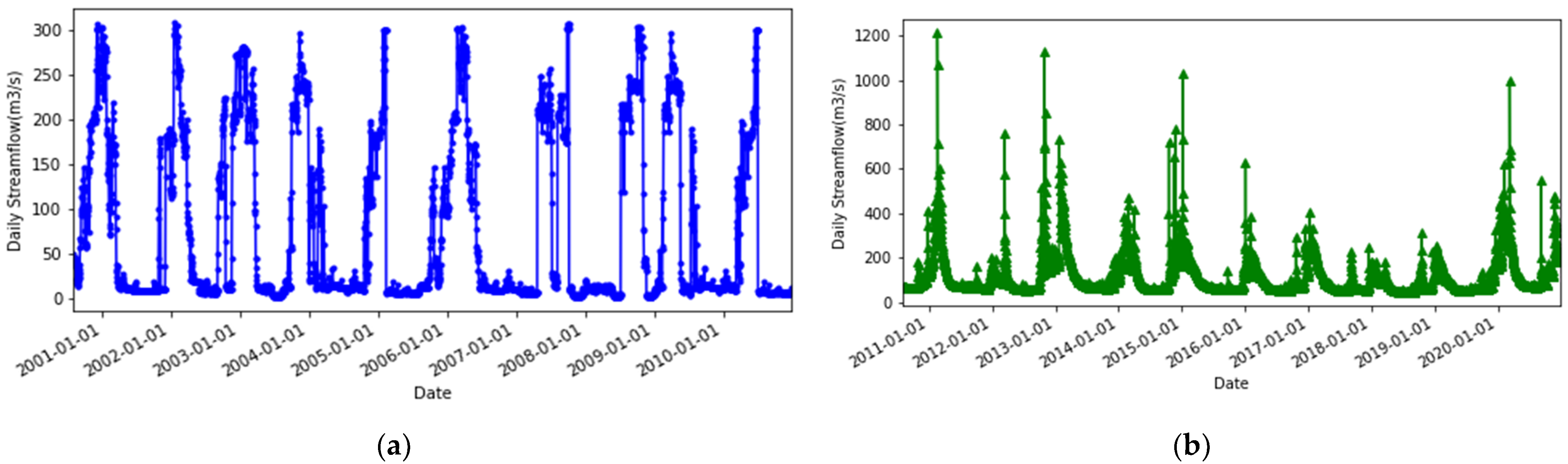
2.1. Study Region

The impacts of climate change in Turkey have been recently manifested in the decreasing trend in precipitation and drought events. One of the basins where the impacts of the change are observed is the Seyhan River Basin. The Seyhan Basin contains a hydrological structure that is sensitive to climate changes, as it is wealthy in surface water resources and is located in the transition zone from the semi-arid climate zone to the continental climate. A river network is well-formed in the basin, and there are numerous karstic water structures in the upper elevations of the basin. For this reason, the Seyhan Basin has been taken as the subject of the study due to its significance in water resources management and planning. Furthermore, the basin was established as a consequence of preliminary studies, that identified it as the most sensitive and vulnerable region to global warming by the Intergovernmental Panel on Climate Change (IPCC) Mediterranean Region. Additionally, the determination of risky regions by employing historical hydrological data on a regional basis is crucial in terms of planning [38].
There are various plans that have been made by the government regarding the basin. The Seyhan Basin Pollution Prevention Action Plan and Seyhan Basin Flood Management Plan are among the studies completed by the General Directorate of Water Management and the General Directorate of Environmental Management [39]. Not only the government, but also numerous researchers, has tackled the basin. Simsek [40] designed a hydrological drought analysis using the Streamflow Drought Index (SDI) method for the Seyhan River Basin. Additionally, Zeybekoglu [41] applied the Standardized Precipitation Evapotranspiration Index (SPEI) for the first time in the Seyhan River Basin. Zerberg and Ozkaya developed a daily reservoir operation model to evaluate the water storage changes in the Seyhan River Basin. On the other hand, Ayten et al. [42] developed a plan for the Seyhan River Basin regarding water allocation among groups of water use or sectors by considering environmental and socio-economic conditions, as well as the potential of surface and groundwater resources.
The Seyhan Basin is shown in Figure 1; its upper part is located in Central Anatolia and the middle and lower parts are located in the Mediterranean Region. The coordination of the basin is between 36°33′–39°12′ N and 34°24′–36°56′ E, and it includes the water catchment areas of Seyhan River and the Göksu and Zamanti branches. It extends to the Ceyhan Basin in the east, the Berdan River in the west, and Develi in the north, which is within the borders of Kayseri, and the entire basin covers an area of approximately 21,000 km2 [43]. In addition, most of the northeastern extensions of the Taurus Mountains are located within the basin, and hold both mountainous and aquatic ecosystems. The Seyhan River is one of Turkey’s largest rivers that flows into the Mediterranean. Its length is 560 km with all its tributaries considered, and the Zamanti and Göksu Rivers and the main contributors. The Seyhan Basin, which begins at the Mediterranean coastline and extends to Central Anatolia, possesses different characteristics in terms of climate within its borders. In the threshold areas of the Çukurova and the Taurus Mountains, summers are hot and dry, and winters are warm and rainy. This region penetrates into the arid–less fertile, excess water climate type [44,45,46].

2.2. Datasets and Pre-Processing

In this study, two flow measurement stations representing various hydrological conditions of the Seyhan River Basin were established to validate the predictive capacity of the generated model. They were selected in accordance with the conditions of being on various branches of the Seyhan River Basin, as shown in Figure 1 [47]. Moreover, the daily flow measurement stations (FMSs) were used to gather long-term 10-year streamflow data. The timespan of the Üçtepe and Tuzla stations included in the study is 2000–2009. The datasets consist of daily flow values.
Üçtepe FMS (E18A018), located at the junction of the two water collection branches of the Seyhan River, is one of the most critical points to be analyzed in terms of its water collection capacity and river flow forecasts. In addition, the Goksu River Sub-Basin, located in the northeast of the Seyhan Basin, has low sensitivity and economic value, and high adaptability. Tuzla FMS (D18A045) is located in the south of the Seyhan Basin in a sub-basin with a coast on the Mediterranean. In spite of the fact that this sub-basin has a high adaptation capacity, it has been determined that it is a sub-basin exposed to drought at a high level due to its high economic value. As a result, it is noticed that the lower Seyhan Plain Sub-basin, which is the sub-basin where agricultural activities are most intense, is the basin that will be highly impacted in the agricultural sector. The locations of the stations on the Seyhan River are shown in Table 1, with their geographical coordinates. As seen in Figure 2, the two river stations’ minimum and maximum flow rates during the observation period were 1.78 m3/s and 30 m3/s, respectively. As regards the streamflows at the FMSs and their daily distributions, as given in Figure 2, the lowest flow rate value for the two stations is at Tuzla station, at 2.3 m3/s, and the highest flow rate value is 1214 m3/s, observed at the Üçtepe station. At Üçtepe FMS, the highest flow rate was observed at 1214 m3/s, and the lowest flow rate was 42.1 m3/s. The highest flow rate in Tuzla FMS was measured as 309 m3/s and the lowest flow rate was 2.3 m3/s.
In the hybrid model created, Python 3.9, one of the versions of the Python programming language, was employed with new components and optimization. Besides this, Keras Library, a high-level artificial neural network library, was utilized in the training and test prediction processes. In the hybrid model consisting of daily flow data, the GRU consisted of 100 periods for training processes and eight batch sizes for performance analysis. ADAMAX was utilized as the RMSE optimizer as the loss function in the study. Additionally, the flow values utilized in the study were constructed with the data collected from EIEI (General Directorate of Electrical Works and Survey Administration) and DSI (Hydraulic State Works). The daily flow data collected from Üçtepe and Tuzla stations had a time span of 10 years (approximately 3650 days). In total, 75% of the data were used as the training set and the remaining 25% as the test set. These data obtained from the stations were trained to compare the models. The linear regression, hybrid model, and the performance of the hybrid model were analyzed for the test data. The hybrid model consisted of three hidden layers and one dense layer.
There is a large amount of missing data at some flow monitoring stations [48]. The missing data indicate significant issues in terms of the proper planning of water resources. Since the measurement of drainage basins is not available or is insufficient worldwide, many reports have been published on the sustainability of water resources [49]. This scientific activity is an effort to enhance flow estimates for unmeasured basins. However, in many basin-based studies, when meteorological data (precipitation, snow, temperature, evaporation, etc.) and hydrological data (flow observation or flow measurement) are obtained from institutions, data on past dates might be missing, as a result of interruptions. The interruption might be due to various reasons, such as climatic difficulties, transportation difficulties, and problems with the measuring device. Since it is not always possible to access flow records when required, attention ought to be paid to ensure that the data are not interrupted, or interrupted are only for a short time. Despite the possible river flow recording gaps, some significant issues may be encountered in terms of operation, sustainability and effective planning. Thus, we retained long-standing uncorrupted flow data in the study to obtain an accurate and prosperous estimation.
In this study, we analyzed historical flow data of stations to predict forthcoming river flows and evaluate proposed models. Accordingly, we included long-standing uninterrupted flow data to receive an accurate estimate. It was vital that the received stream data were documented completely and not interrupted. At this stage, short interruptions in flow data were tolerated. The formation of gaps in the flow data due to adverse climatic conditions or other reasons create critical issues in terms of effective planning, design, and operation. In addition, these conditions should be taken into account in determining the flow values so that the structure and hydrological characteristics among the datasets are not deteriorated.

2.3. Methods

2.3.1. Gated Recurrent Unit

The LSTM and GRU models are deep-learning models based on RNN that have been widely operated in the last few years for streamflow forecasting. LSTM was initially presented in 1997, and it is capable of learning long-short term variables [50]. However, LSTM has three gating layers in each module and encloses a complex structure. Accordingly, the training process for the development of LSTM neural networks generally takes a long time. The GRU algorithm was first proposed by Cho et al. to overcome these drawbacks as a simpler variant of LSTM. Both algorithms contain a similar structure and can produce equivalent qualified outcomes [51,52]. Some studies investigated their performances by comparing the GRU and LSTM models for streamflow prediction [53]. It was noted that the prediction accuracy of these models was increased and stabilized with larger time steps, while the GRU model functioned better than LSTM. It has been seen that the GRU can be utilized for short-term flow forecasting, since it demands less time for training [54].
zt = σ (wz · [h (t − 1), xt])
rt = σ (wr · [h (t − 1), xt])
ht = tanh (w · [rth(t − 1), xt])
The typical structure of the GRU model is displayed in Figure 3. The GRU architecture has two gating layers called the update gate (zt), (Equation (1)) which combines the input gate and forget gate of LSTM, and the reset gate (rt), which is the output gate in LSTM. The reset gate (rt) is used from the model to determine how much of the past information must be neglected. The formula is the same as that for the update gate. There is a dissimilarity in their weights and gate usage, which is indicated in Figure 4. The update gate functions as the forget and input gates in the LSTM algorithm, controlling the degree of information brought to the current time step from the previous step. In order to obtain more state information from the previous time (t − 1) to the current time step (t), the value of the update gate must be large. The reset gate, which is mentioned in Equation (2), specifies how much of the memory to let through [55]. The smaller the reset gate (rt), the less information reported from the previous state. Here, (xt) is the input vector served in the network unit. It is multiplied by its parameter weight (w) matrices. The (t − 1) in h(t − 1) signifies that it holds the information of the previous unit, and it is multiplied by its weight. Then, the values from these parameters are added and passed through the sigmoid activation function. The sigmoid function would generate values between 0 and 1 at this step. At the current time step, the network needs to calculate (ht) in the final memory, in which process the update gate will play a vital role. This vector value will maintain information for the current unit and pass it down to the network. It will determine which information to collect from the current memory content (ht) and previous timesteps h(t − 1), which are stated in Equation (3). The output of the product is used in the input via point-wise addition with (ht), to produce the final results in the hidden state.

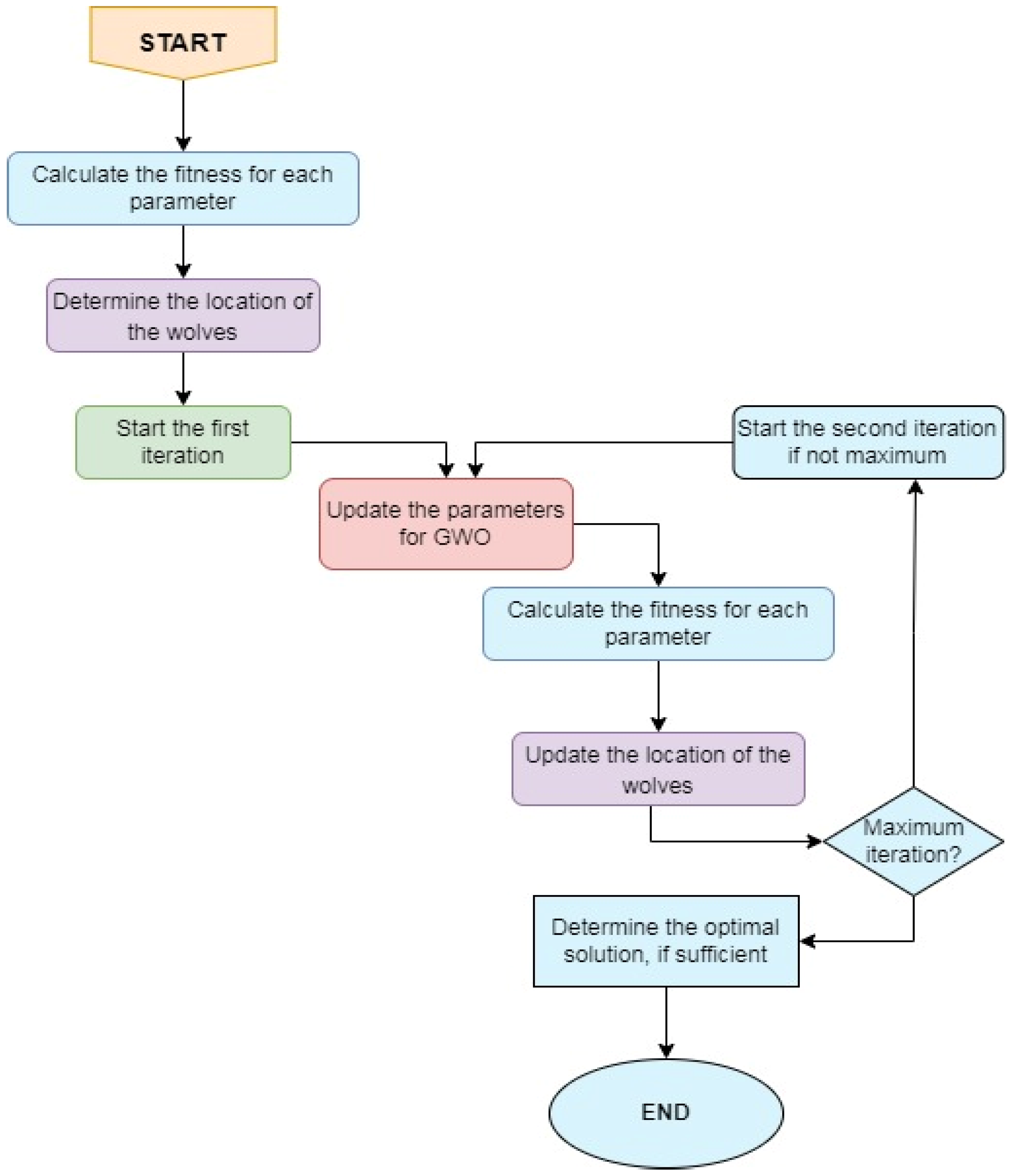
2.3.2. Grey Wolf Optimization

The grey wolf optimization (GWO) is defined as a swarm intelligence optimization model, and it offers several benefits, i.e., flexibility, simplicity, and a non-derivative mechanism. Additionally, it has a limited control agent to adjust, and superior convergence. Some studies have found that GWO has better numerical characteristics that enable it to prevent local optimum compared to other traditional optimization models, and it has been suggested as a convenient stochastic method to solve highly nonlinear, multivariate and multimodal optimization problems [56]. GWO, a novel metaheuristic algorithm technique, was initially proposed by Mirjalili et al. [57], and was inspired by grey wolves’ hunting and social hierarchy. A grey wolf pack is intrinsically divided into four ranks, which are named alpha (α), beta (β), delta (σ) and omega (Ω). The top level of the hierarchy is alpha, the prevailing leader wolf of the pack. Additionally, crucial determinations are made by the alpha grey wolves. The second rank of the grey wolves’ hierarchy is the beta wolves, which serve as mentors and provide feedback to empower and assist the alpha wolf. Delta wolves, on the other hand, obey the orders of the alpha and beta wolves, and rule over omega wolves. Finally, omega wolves are the lowest group in the hierarchy and follow the other dominant wolves. The primary stages of the grey wolf hunting process contain hunting, encircling and attacking the prey [58]. In the GWO algorithm, the hierarchy is structured as the fittest solution, the second-best solution, the third-best solution, and the rest of the candidate solutions [59]. Encircling the prey in the hunting process is represented by the following equations (Equations (4) and (5)):
D   = | C   ·   X   p ( t ) X   ( t ) |
X     ( t + 1 ) = X   p ( t ) A   ·   D  
where D represents the interaction between the prey and grey wolf, t is the current iteration, Xp(t) and X are the position vectors of the prey and grey wolf in iteration, respectively. A and C indicate parameter vectors, and these coefficient vectors are computed according to the equations given below (Equations (6) and (7)).
A   i = 2 a     r   i 1 a   , i = α ,   β ,   δ
C   i = 2 r   i 2 ,   i = α ,   β ,   δ
where α is the linearly decreasing vector from 2 to 0, and r   i 1   and r   i 2   indicate randomly generated vectors in [0, 1], respectively.
The flowchart of the GWO algorithm is presented in Figure 4 to understand better how GWO functions.

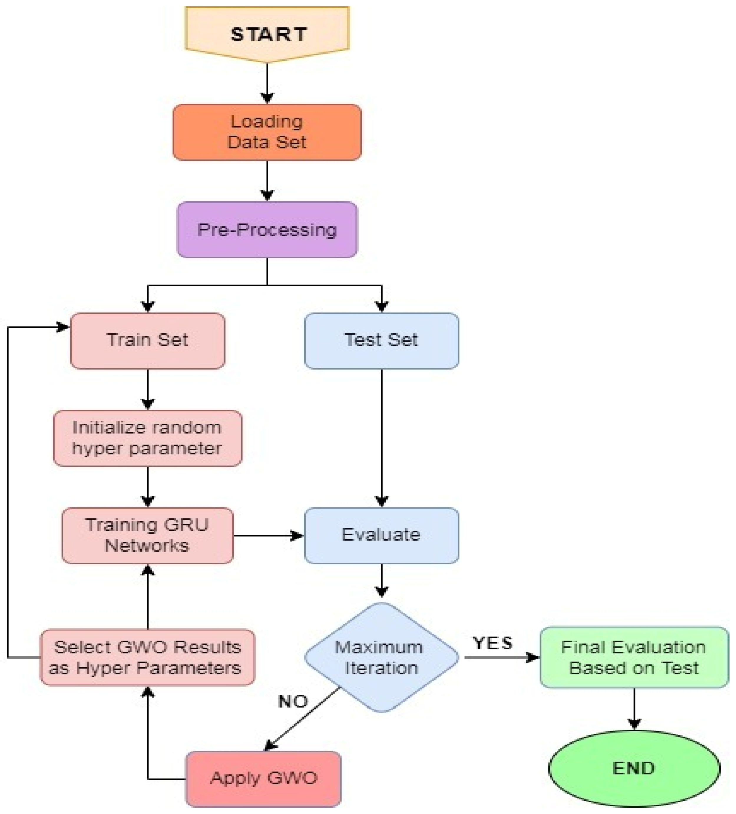
2.3.3. Predicting of Streamflow Based on GWO-GRU (Proposed) Model

The GRU is a deep learning model, and is a variant of LSTM. It is more rapid, as less computation is required to update its hidden state. According to LSTM, the benefit of the GRU reaches the fore when considering its abilities, such as swiftly optimizing the basic parameters and the initial values of the parameters. In addition, the GRU network has fewer hyperparameters than LSTM, so it is quicker to train and needs less information for training.
There may be various hyperparameter groups wherein the model provides satisfactory performance. It is unnecessary to use each of these groups in model design. However, determining the most appropriate hyperparameter group is one of the vital concerns to address. The selection of hyperparameters is commonly based on the designer’s intuition, the experience gained from previous situations, reflections on applications in various fields, current trends, and design dependency within the model. However, lately, various strategies have been put forward to determine the most suitable hyperparameter group that is best suited to finding the solution to the problem. The size of the dataset, the learning coefficient, the activation function, the learning rate, and the momentum coefficient are adjustable parameters that allow the model’s training process to be controlled. Hence, optimal conditions have been sought by optimizing several hyperparameters of the GRU model with GWO. In this process, the GWO algorithm, whose results were determined, was added to the GRU network as a parameter, and the model was retrained. Then, the results were compared with the benchmark model. After that, the test results were compared by training fifteen times, and the most promising results were determined as the benchmark model. The accuracy and performance of the results were compared via linear regression, which is a physical-based method, as well as the comparison model, and the success of the models in the flow predictions was observed. The dataset is trained with the data via machine learning, and particularly supervised learning. The systematics of machine learning models are as follows: the dataset is divided into training and test sets. ML models are trained with some of the data, and are expected to make accurate predictions from untrained, unpredictable data. That is, the model comprehends the data, and presents results using what it has learned from other datasets. The suitability and feasibility of the training are also verified with test data, and it is decided whether the model is usable or not. Putting all of the data into the models requires both getting proper results and waiting a long time for the codes to run. For this reason, the dataset is divided as 70% training, 30% testing, 75% training, 25% testing, and finally 80% training and 20% testing. The most successful results from training the network were obtained when the data were separated as 75% training and 25% testing. This is why this ratio was used in the study.
Afterwards, the GRU network was trained with two dense and two GRU layers, so that the network structure contained four hidden layers. After altering the window size and number of neurons in the two GRU layers, the network was run five times, and the most successful results of the four-hidden layer network were obtained as benchmark results. Subsequently, the GWO algorithm was designed, and its results determined the GRU model window size and the number of neurons. The GWO parameters were set as follows:
Number of grey wolves = 50; number of maximum iterations = 100; lower bound = −20; upper bound = 20; number of dimensions = 3; fitness function = GRU model execution. The RMSE results of the GRU network in training were used as the fitness value, so the model was hybridized.
As seen in Figure 5, while creating the model, the dataset was first loaded, and pre-processes were applied. In this way, the dataset was made trainable and workable. Then, the dataset was divided into 75% for training and 25% for testing. The training data were first trained with randomly determined hyperparameters, and their success was evaluated on the test data. Next, the GWO algorithm was applied, and the results were used as hyperparameters (number of neurons and window size). After that, the network was retrained, and its success in the test dataset was determined by the RMSE measurement method. The same process was repeated until the end of the iteration, and the best results were compared with the results from the training of the network using randomly determined hyperparameters.

3. Results

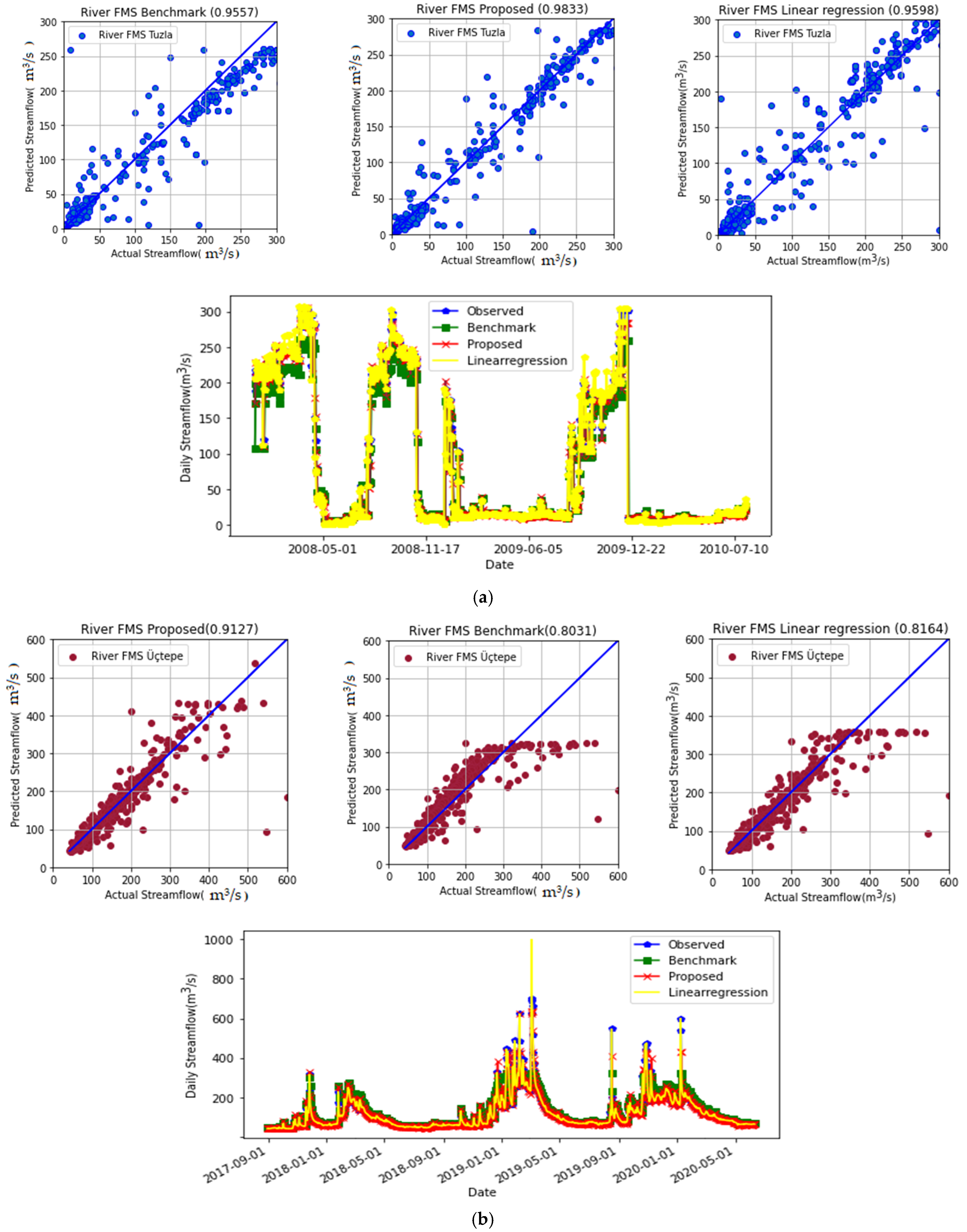
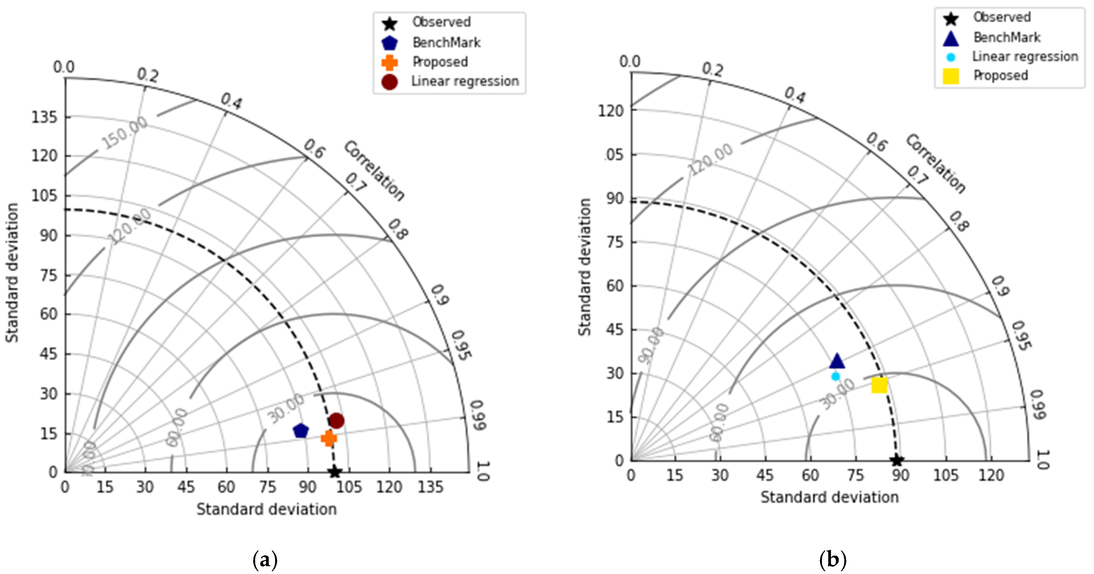
3.1. Performance Evaluation of Models

Forecasting evaluation criteria and FMS model results of the two study stations are given in Table 2 and Figure 6, respectively. In this paper, the RMSE, MAPE, MAE and SD statistical indexes were employed to evaluate the forecasting performance of the GRU, GWO and linear regression models. The linear regression model is used to predict the future when a linear relationship is observed between the variables, to examine how the variables affect each other, and to make inferences. These statistical indexes have been commonly put to use in hydrological evaluation models to assess daily flow values [60].
As shown in Table 2, for both the Üçtepe and the Tuzla FMS, the best results were obtained via the proposed GWO–GRU hybrid model. In the Üçtepe FMS, the lowest RMSE, MAE, MAPE and SD values were obtained via the GWO–GRU hybrid model, with the highest accuracy (R2 = 0.9127) being 82.93 m3/s, 85.93 m3/s and 62.48 m3/s, respectively. In the GRU and linear regression models, the R2 values (0.8031 and 0.8164, respectively) were found to be lower than in the proposed model, and similarly, the RMSE values (124.57 and 120.54 m3/s, respectively) and MAE values (184.06 and 107.94 m3/s, respectively) were higher compared to the hybrid model. The same trend was observed for the Tuzla FMS, and according to the comparison of these three models’ predictions, while the R2 values of the GRU and linear regression were 0.9557 and 0.9598, respectively, this value increased to 0.9833 in the proposed model. As a result, the proposed model provided better RMSE, MAE, MAPE and SD values than the other two benchmark models. When the values given in Table 2 are analyzed, while the predicted RMSE of the proposed model was 13.16 m3/s, the predicted RMSE values of the GRU and linear regression models were 21.12 m3/s and 19.98 m3/s. Similar to the RMSE results, the trend in the MAE results was assessed via the same method as was used for the GWO–GRU model (5.13 m3/s), which result was lower than those of the GRU and linear regression models (10.79 m3/s and 8.24 m3/s, respectively). Additionally, the MAPE gave more reasonable results than the other models. As demonstrated in Table 2, it is apparent that the proposed model produced highly successful predictions for the other algorithms at both of the two FMSs. In addition to the statistical indexes, the proposed river FMS benchmark and linear regression results for both FMSs are presented in Figure 6. The scatter plots for the three models compare the correlation between the real and predicted streamflow data. As stated earlier, the correlation between actual and predicted streamflow can be seen more clearly in the figure. It has been monitored that the distribution of the proposed model was more pleasing than the other algorithms, and the R2 values of the proposed model were higher for both FMSs than with the benchmark and linear regression models. In addition to this, it was noticed that the actual and predicted streamflow data in the distribution, primarily after the flow of 175 m3/s, were rather compatible with each other at the Tuzla FMS (Figure 6a). It is clear that there is a more diffuse structure in the scatter plots of the other models. At the Üçtepe FMS, on the other hand, the distribution between 0 and 300 m3/s was more correlated with the actual and predicted data (Figure 6b). After 300 m3/s, although the correlation deteriorated for all three models, the deterioration in the proposed model was less than that in the others. The results indicate that the proposed hybrid model achieved the best performance in estimating the streamflow at the studied FMS.

3.2. Comparative Analysis and Discussion

Figure 7 gives the standard deviation and correlation data via a Taylor diagram. The indicated diagram includes the benchmark, hybrid, and linear regression models’ results. The Taylor diagram, which includes many parameters, was used to evaluate the river flow estimates with further statistical analysis. It provides a graphic summary of how close the models are to the observations, and evaluates the similarity, correlations, centripetal mean square roots, and the change magnitudes between the two models [61]. When the Taylor diagram was investigated for both stations, the success of the hybrid model was clear. The hybrid model provided the closest results to the observed values at the Üçtepe station. The linear regression model and the GRU network lagged behind the hybrid model at this station. When the results for Tuzla station were analyzed, the hybrid model offered better accuracy than both models individually. In this station, the linear regression model performed better than the benchmark model. The hybrid model with the Taylor diagram displayed a higher success rate, in addition to better statistical parameters.
Together with the other results, the success and accuracy of the hybrid model was assessed via the statistical measurement metrics with other studies in this field. Tikhamarine et al. [62] utilized a hybrid model with an integrated GWO algorithm to enhance monthly flow estimation and SVR accuracy. The hybrid model has been compared with other algorithms. The outcomes demonstrate that the GWO algorithm outperformed other algorithms in terms of both prediction accuracy and convergence. Kohli and Arora [63] introduced chaos theory to the GWO algorithm in order to accelerate the rate of global convergence. The performance of the newly formed hybrid model has shown various engineering design issues. The results indicate that, with a suitable chaotic map, the hybrid model could apparently outperform the standard GWO, with very good performance compared to other algorithms. Oudira et al. [64] analyzed the impacts of different ratios on the grey wolf optimization model. The outcomes reveal that the new GWO scheme outperforms the detection methods mentioned in the literature in most cases. Liu et al. [65] developed a new artificial neural network and deep learning model, the binary grey wolf echo state network. The performance of the developed hybrid model was analyzed using different datasets. The results illustrate that the proposed model was more effective than other benchmarking models, and achieved the lowest error rate. Ozsoydan [66] analyzed the effects of dominant wolves, which have crucial effects on the search capability of the GWO, and introduced new extensions based on variations in dominant wolves. The performances of all algorithms developed with the mentioned new extensions have been tested. The proposed modifications were compared with the standard GWO, Particle Swarm Optimization. The results of this study exhibit those dominant wolves had noteworthy effects on the performance of the GWO. Song et al. [67] compared GWO with some other well-known stochastic search algorithms, including GA and PSO, in the parameter estimation of surface waves. Regarding the obtained results, the authors strongly recommend the use of GWO. Daniel et al. [68] developed a new hybrid model using two metaheuristic algorithms: the grey wolf and the cuckoo search algorithms. Models were analyzed with various performance measures. The results reveal that the employed hybrid model presented more satisfactory results than conventional separation techniques.
When the results obtained from the methods applied in the study are examined in detail, it is extremely critical to integrate the GWO algorithm into the GRU model. In the original GWO algorithm, after the update, one must checked whether the positions of the wolves exceed the search space limits. If the new location of the grey wolf exceeds the upper or lower limits, the location of the grey wolf is equalized to the limit value so that the boundary conditions are not exceeded. This is very common in the discovery phase. For this reason, many wolves can get stuck at the boundaries of the search space in some cases. Developable features, such as convergence and searching, which are common in the grey wolf algorithm and an integrated algorithm structure, have successfully estimated the optimal river flow values at both stations. All in all, as can be seen from the datasets obtained from the two stations (Table 2 and Figure 6), the designed hybrid GWO–GRU model was successful in all statistical measurements at both stations, except for the standard deviation value of the linear regression model at Tuzla station. The closest evaluation criterion to the hybrid model at Üçtepe station is the standard deviation value of the linear regression model. However, at this station, the hybrid model outperformed other models. As a result, it is clear from the analysis performance that a model strengthened with the GWO algorithm for convergence and prediction parameters achieves the best results. In addition to the hyperparameters applied in the study, new methods (especially a new local search) or models that can be constructed by integrating them into the proposed model using a different metaheuristic algorithm will guide future studies. In addition, the ever-increasing innovation of deep learning and nature-inspired metaheuristic algorithms will enable these integrated models to be even more powerful.

4. Conclusions

In river flow forecasting studies, optimization algorithms are also operated in the process of obtaining the best flow estimation. In recent years, many optimization algorithms inspired by nature, especially imitating animal behavior, have been developed and successfully applied to many engineering issues. Some of them include Particle Swarm Optimization (PSO), Cuckoo Optimization (CO), Bee Colony Optimization (BCO), and the White Whale Optimization (WWO) algorithm. In the literature, it has been stated that one of the most successful of these algorithms is GWO [69]. In this study, a GWO variant named the GWO–GRU algorithm, which is delivered as a multi-strategy random weighted approach of the GWO algorithm, is proposed. A new integrated model combining the grey wolf optimization (GWO) algorithm and the gated recurrent unit (GRU) is proposed to predict daily flow in the Seyhan basin. The GWO was designed to optimize the hyperparameters of the GRU, such as the global solution parameters, and was then compared with the Linear regression model. The performance of the generated hybrid model has been extensively analyzed based on the different statistical parameter results of two flow measurement stations located in different catchment areas of the Seyhan basin [70]. In this study, the GWO–GRU hybrid model yielded R2 = 0.9127, RMSE = 82.9352 m3/s, MAE = 85.9337 m3/s and MAPE = 62.4796 m3/s, whereas the linear regression forecasting produced the following results: R2 = 0.8164, RMSE = 120.5431 m3/s, MAE = 107.9480 m3/s and MAPE = 72.6310 m3/s for Üçtepe FMS. According to these results, the RMSE decreased by 3%, and thye R2 was almost 12% better than the linear regression. Similarly, when Tuzla FMS data were used as inputs for the models, better results were obtained in the proposed model compared to the linear regression model. The RMSE, MAE and MAPE decreased by approximately 34%, 37% and 73%, respectively, while the coefficient R2 was increased by about 2.5%. First, convergence, search history, trajectory and mean distance analyses, and comparisons with classical estimation methods, are provided. These analyses have focused on the issue of river flow forecasting, which was considered a fundamental concern in the world and is used in the literature. As a result of the convergence analysis, it was seen that the GWO–GRU algorithm converged faster than the GWO algorithm in solving the problem. The ability of the proposed GWO–GRU algorithm to find a solution closer to the global optimum as noticed. The search history analysis outcomes indicate that the distribution of grey wolves around the global optimum updated by the hybrid model is higher than the distribution of grey wolves. In addition, the exploration and exploitation stages and the search space have been updated by the GWO algorithm. The grey wolves that were encountered by the GWO algorithm were stuck in the boundary values of the search space, particularly on the surfaces of the benchmark problems during the search history analysis [71]. According to the trajectory analysis results of the GWO–GRU algorithm, the position of the alpha wolf was updated faster during the exploration phase, and approached the global optimum during the exploitation phase. The proposed GWO–GRU algorithm successfully avoids the local optimum points of the issue in the parts that expand the mean distance curve of the GWO–GRU algorithm during the exploration phase. According to the results obtained from the basic statistical measurement metrics, the tests on the benchmark model and the classical estimation model illustrate that the GWO–GRU algorithm is promising. In the comparison, the GWO algorithm produced better solutions for time series problems. Therefore, the approach that we developed with the GWO algorithm can be suggested as an alternative algorithm to be used in time series problems. As is well-known, streamflow forecasting is important for sustainable water management. The knowledge and data obtained with streamflow forecasting were used especially in designing water infrastructures, flood alerts and more effective water management [72]. It can be concluded that the results obtained with the GWO–GRU hybrid model for both FMSs significantly extend the accuracy of the streamflow forecasts in the monthly time scales, compared to the results obtained with the single models. Therefore, it can be considered that the proposed hybrid model may be a promising model for modeling monthly flows. Thus, the results obtained in this study with a new approach show that machine learning methods can be successfully applied as an alternative for the abovementioned purposes, such as to design water infrastructures, determine river behavior and construct flood control measures.
However, the study has some limitations. In this study, only flow data were utilized as the input. The generated hybrid model was evaluated only for daily streamflow. In future studies, many parameters, such as humidity, snowmelt, and temperature can be used. Furthermore, the model can include decomposition techniques, since the data are non-linear. Other hydrological variables can be applied in the field of hydrology to examine the proposed model. In future studies, innovations such as increasing the number of objective functions and the harmonic system can be made by taking the problem constants as variables or modeling closer to reality. By using different methods in the distance calculation process of the algorithms, the most suitable method to improve the performance of the algorithms can be determined. Thus, the performance of algorithms can be increased. In addition to the global search algorithm, a new hybrid model can be constructed with the local search algorithm, and the performance of the model can be analyzed. However, the comparison model can also be hybridized with other recently popularized algorithms (for example, a meta-heuristic algorithm based on the intelligent behavior of crows, called the Crow Search Algorithm (CSA)), and the contributions of the two algorithms to prediction accuracy can be examined. The high accuracy of the developed hybrid model, used for river flow estimations, will enable the model to be developed further in future with different input parameters.

Author Contributions

H.C.K. and A.Y. prepared the original draft, and reviewed and improved the manuscript. All authors have read and agreed to the published version of the manuscript.

Funding

This research did not receive any funding.

Institutional Review Board Statement

Not applicable.

Informed Consent Statement

Not applicable.

Data Availability Statement

Not applicable.

Conflicts of Interest

The authors declare no conflict of interest.

Abbreviations

ANNArtificial Neural Networks
DLDeep Learning
DSIHydraulic State Works
EIEIElectrical Works Survey Administration General Directorate
FMSFlow Measurement Station
GRUGated Recurrent Unit
LSTMLong Short-Term Memory
MAEMean Absolute Error
MAPEMean Absolute Percentage Error
MSEMean Square Error
GAGenetic Algorithm
ACAAnt Colony Algorithm
PSOParticle Swarm Optimization
ABCArtificial Bee Colony
DEADifferential Evaluation Algorithm
COCuckoo Optimization
CSACrow Search Algorithm
GWOGrey Wolf Optimization
WWOWhite Whale Optimization
WSOWeighted Superposition Optimization
FOForest Optimization
SASimulation Annealing
IPCCIntergovernmental Panel on Climate Change
BCOBee Colony Optimization
RMSERoot Mean Square Error
RNNRecurrent Neural Networks
SDStandard Deviation

References

  1. Makkeasorn, A.; Chang, N.B.; Zhou, X. Short-term streamflow forecasting with global climate change implications—A comparative study between genetic programming and neural network models. J. Hydrol. 2008, 352, 336–354. [Google Scholar] [CrossRef]
  2. Mishra, A.K.; Singh, V.P. A review of drought concepts. J. Hydrol. 2010, 391, 202–216. [Google Scholar] [CrossRef]
  3. Kilinc, H.C.; Haznedar, B. A Hybrid Model for Streamflow Forecasting in the Basin of Euphrates. Water 2022, 14, 80. [Google Scholar] [CrossRef]
  4. Zealand, C.M.; Burn, D.H.; Simonovic, S.P. Short term streamflow forecasting using artificial neural networks. J. Hydrol. 1999, 214, 32–48. [Google Scholar] [CrossRef] [Green Version]
  5. Wang, W.C.; Chau, K.W.; Cheng, C.T.; Qiu, L. A comparison of performance of several artificial intelligence methods for forecasting monthly discharge time series. J. Hydrol. 2009, 374, 294–306. [Google Scholar] [CrossRef] [Green Version]
  6. Myronidis, D.; Ioannou, K.; Fotakis, D.; Dörflinger, G. Streamflow and hydrological drought trend analysis and forecasting in Cyprus. Water Resour. Manag. 2018, 32, 1759–1776. [Google Scholar] [CrossRef]
  7. Krajewski, W.F.; Ghimire, G.R.; Quintero, F. Streamflow Forecasting without Models. J. Hydrometeorol. 2020, 21, 1689–1704. [Google Scholar] [CrossRef]
  8. Nourani, V.; Baghanam, A.H.; Adamowski, J.; Kisi, O. Applications of hybrid wavelet–Artificial Intelligence models in hydrology: A review. J. Hydrol. 2014, 514, 358–377. [Google Scholar] [CrossRef]
  9. Londhe, S.; Charhate, S. Comparison of data-driven modelling techniques for river flow forecasting. Hydrol. Sci. J. 2010, 55, 1163–1174. [Google Scholar] [CrossRef]
  10. Yaseen, Z.M.; El-shafie, A.; Jaafar, O.; Afan, H.A.; Sayl, K.N. Artificial intelligence-based models for stream-flow forecasting: 2000–2015. J. Hydrol. 2015, 530, 829–844. [Google Scholar] [CrossRef]
  11. Zhang, Z.; Zhang, Q.; Singh, V.P. Univariate streamflow forecasting using commonly used data-driven models: Literature review and case study. Hydrol. Sci. J. 2018, 63, 1091–1111. [Google Scholar] [CrossRef]
  12. Fathian, F.; Mehdizadeh, S.; Kozekalani Sales, A.; Safari, M.J.S. Hybrid models to improve the monthly river flow prediction: Integrating artificial intelligence and nonlinear time series models. J. Hydrol. 2019, 575, 1200–1213. [Google Scholar] [CrossRef]
  13. Tikhamarine, Y.; Souag-Gamane, D.; Ahmed, A.N.; Kisi, O.; El-Shafie, A. Improving artificial intelligence models accuracy for monthly streamflow forecasting using grey Wolf optimization (GWO) algorithm. J. Hydrol. 2020, 582, 124435. [Google Scholar] [CrossRef]
  14. Türkşen, Ö.; Akgün, F. Genetik-Simpleks hibrit algoritması ile doğrusal olmayan regresyon model parametrelerinin nokta tahmini. J. Stat. Stat. Actuar. Sci. 2018, 2, 81–92. [Google Scholar]
  15. Chen, Y.; Song, L.; Liu, Y.; Yang, L.; Li, D.A. Review of the Artificial Neural Network Models for Water Quality Prediction. Appl. Sci. 2020, 10, 5776. [Google Scholar] [CrossRef]
  16. Ebrahimi, S.; Esfandiari, M.; Ahmadi, A. Efficiency of Regression, ANN and ANN-algorithm Genetic Hybrid Models in the Evaluation of Wind Erosion. J. Water Soil Resour. Conserv. 2022, (in press). [Google Scholar]
  17. Han, S.; Meng, Z.; Zhang, X.; Yan, Y. Hybrid Deep Recurrent Neural Networks for Noise Reduction of MEMS-IMU with Static and Dynamic Conditions. Micromachine 2021, 12, 214. [Google Scholar] [CrossRef] [PubMed]
  18. Karim, M.E.; Maswood, M.M.S.; Das, S.; Alharbi, A.G. BHyPreC: A Novel Bi-LSTM Based Hybrid Recurrent Neural Network Model to Predict the CPU Workload of Cloud Virtual Machine. IEEE Access 2021, 9, 131476–131495. [Google Scholar] [CrossRef]
  19. Karijadi, I.; Chou, S.Y. A hybrid RF-LSTM based on CEEMDAN for improving the accuracy of building energy consumption prediction. Energy Build. 2022, 259, 111908. [Google Scholar] [CrossRef]
  20. Cho, K.; Van Merriënboer, B.; Gulcehre, C.; Bahdanau, D.; Bougares, F.; Schwenk, H.; Bengio, Y. Learning phrase representations using RNN encoder-decoder for statistical machine translation. In Proceedings of the 2014 Conference on Empirical Methods in Natural Language Processing (EMNLP), Doha, Qatar, 25–29 October 2014; Association for Computational Linguistics: Stroudsburg, PA, USA, 2014; pp. 1724–1734. [Google Scholar]
  21. Garip, Z.; Çimen, M.E.; Boz, A.F. An Enhanced Chaotic Based Whale Optimization Algorithm for Parameter Extraction of Photovoltaic Models. J. Polytech. 2021, 154, 113018. [Google Scholar]
  22. Çelik, Y.; Yıldız, İ.; Karadeniz, A.T. A Brief Review of Metaheuristic Algorithms Improved in the Last Three Years. Eur. J. Sci. Technol. 2019, 463–477. [Google Scholar] [CrossRef]
  23. Durgut, R.; Aydın, M. Adaptive binary artificial bee colony for multi-dimensional knapsack problem. J. Gazi Univ. Fac. Eng. Archit. 2021, 36, 2333–2348. [Google Scholar]
  24. Haznedar, B.; Arslan, M.T.; Kalinli, A. Optimizing ANFIS using simulated annealing algorithm for classification of microarray gene expression cancer data. Med. Biol. Eng. Comput. 2021, 59, 497–509. [Google Scholar] [CrossRef]
  25. Avuçlu, D.; Ekmekci, D. Geleceğin Dünyasında Bilimsel ve Mesleki Çalışmalar, Bilgisayar Mühendisliği/I.; Ekin Yayinevi: Ankara, Turkey, 2020; ISBN 978-625-7983-95-2. [Google Scholar]
  26. Koc, I.; Baykan, O.K.; Babaoglu, I. Multilevel image thresholding selection based on grey wolf optimizer. J. Polytech. 2018, 21, 841–847. [Google Scholar]
  27. Guimarães Santos, C.A.; Silva, G.B. Daily streamflow forecasting using a wavelet transform and artificial neural network hybrid models. Hydrol. Sci. J. 2013, 59, 312–324. [Google Scholar] [CrossRef]
  28. Štravs, L.; Brilly, M. Development of a low-flow forecasting model using the M5 machine learning method. Hydrol. Sci. J. 2007, 52, 466–477. [Google Scholar] [CrossRef]
  29. Khosravi, K.; Miraki, S.; Saco, P.M.; Farmani, R. Short-term River streamflow modeling using Ensemble-based additive learner approach. J. Hydro-Environ. Res. 2021, 39, 81–91. [Google Scholar] [CrossRef]
  30. Zhao, X.; Lv, H.; Wei, Y.; Lv, S.; Zhu, X. Streamflow Forecasting via Two Types of Predictive Structure-Based Gated Recurrent Unit Models. Water 2021, 13, 91. [Google Scholar] [CrossRef]
  31. Wegayehu, E.B.; Muluneh, F.B. Multivariate Streamflow Simulation Using Hybrid Deep Learning Models. Comput. Intell. Neurosci. 2021, 2021, 5172658. [Google Scholar] [CrossRef]
  32. Negi, G.; Kumar, A.; Pant, S.; Ram, M. GWO: A review and applications. Int. J. Syst. Assur. Eng. Manag. 2021, 12, 1–8. [Google Scholar] [CrossRef]
  33. Mahmoudi, N.; Majidi, A.; Jamei, M.; Jalali, M.; Maroufpoor, S.; Shiri, J.; Yaseen, Z.M. Mutating fuzzy logic model with various rigorous meta-heuristic algorithms for soil moisture content estimation. Agric. Water Manag. 2022, 261, 107342. [Google Scholar] [CrossRef]
  34. Emami, S.; Parsa, J. Optimal Design of River Groynes using Meta-Heuristic Models. Environ. Water Eng. 2022, 8, 146–160. [Google Scholar]
  35. Abdelkader, E.M.; Al-Sakkaf, A.; Elshaboury, N.; Alfalah, G. Hybrid Grey Wolf Optimization-Based Gaussian Process Regression Model for Simulating Deterioration Behavior of Highway Tunnel Components. Processes 2022, 10, 36. [Google Scholar] [CrossRef]
  36. Uzlu, E. Estimates of greenhouse gas emission in Turkey with grey wolf optimizer algorithm-optimized artificial neural networks. Neural Comput. Appl. 2021, 33, 13567–13585. [Google Scholar] [CrossRef]
  37. Jung, S.; Moon, J.; Park, S.; Hwang, E. An Attention-Based Multilayer GRU Model for Multistep-Ahead Short-Term Load Forecasting. Sensors 2021, 21, 1639. [Google Scholar] [CrossRef] [PubMed]
  38. Cavus, Y.; Aksoy, H. Spatial Drought Characterization for Seyhan River Basin in the Mediterranean Region of Turkey. Water 2019, 11, 1331. [Google Scholar] [CrossRef] [Green Version]
  39. Su Yönetimi Genel Müdürlüğü. Seyhan Havzası Sektörel Su Tahsis Planı Hazırlanması Projesi; Impact of Climate Change on Water Resources Project; Ankara, Turkey. 2016. (In Turkish). Available online: https://www.tarimorman.gov.tr/SYGM/Belgeler/asi%20ve%20Seyhan%20kurakl%C4%B1k%20%20%C3%A7ed%20taslak/Seyhan_Havzasi_Taslak_SCD_Raporu_rev(1).pdf (accessed on 8 February 2022).
  40. Simsek, O. Hydrological drought analysis of Mediterranean basins, Turkey. Arab. J. Geosci. 2021, 14, 2136. [Google Scholar] [CrossRef]
  41. Zeybekoglu, U. Spatiotemporal analysis of droughts in Hirfanli Dam basin, Turkey by the Standardised Precipitation Evapotranspiration Index (SPEI). Acta Geophys. 2022, 128, 1–11. [Google Scholar] [CrossRef]
  42. Ayten, N.; Değirmencioğlu, S.; Kimence, T. Planning of Sectoral Water Allocation: A case study of Seyhan River Basin. Turk. J. Water Sci. Manag. 2017, 2, 48–61. [Google Scholar] [CrossRef]
  43. TUBITAK. Havza Koruma Eylem Planları-Seyhan Havzası; Water Management and Preparation of Basin Protection Action Plans; The Scientific and Technological Research Council of Turkey (TUBITAK); Marmara Research Center (MAM) (TUBITAK): Ankara, Turkey, 2010. [Google Scholar]
  44. İrvem, A.; Topaloğlu, F.; Uygur, V. Estimating spatial distribution of soil loss over Seyhan River Basin in Turkey. J. Hydrol. 2007, 336, 30–37. [Google Scholar] [CrossRef]
  45. Chan, C. Property rights and climate change vulnerability in Turkish forest communities: A case study from Seyhan River Basin, Turkey. Clim. Dev. 2013, 5, 1–13. [Google Scholar] [CrossRef]
  46. Ozkaya, A.; Zerberg, Y. Water storage change assessment in the Seyhan Reservoir (Turkey) using HEC-ResSim model. Arab. J. Geosci. 2021, 14, 504. [Google Scholar] [CrossRef]
  47. Turhan, E.; Kallis, G.; Zografos, C. Power Asymmetries, Migrant Agricultural Labour and Adaptation Governance in Turkey: A Political Ecology of Double Exposures; Wiley: Hoboken, NJ, USA, 2019. [Google Scholar]
  48. Yılmaz, M.U. Improvement of Streamflow Estımatıon in Ungauged Basıns. Ph.D. Thesis, Istanbul Technical University, Istanbul, Turkey, 2020. [Google Scholar]
  49. Sivapalan, M.; Takeuchi, K.; Franks, S.W.; Gupta, V.K.; Karambiri, H.; Lakshmi, V.; Liang, X.; McDonnell, J.J.; Mendiondo, E.M.; O’Connell, P.E.; et al. IAHS decade on predictions in ungauged basins (PUB), 2003–2012: Shaping an exciting future for the hydrological sciences. Hydrol. Sci. J. 2003, 48, 857–880. [Google Scholar] [CrossRef] [Green Version]
  50. Hochreiter, S.; Schmidhuber, J. Long short-term memory. Neural Comput. 1997, 9, 1735–1780. [Google Scholar] [CrossRef] [PubMed]
  51. Chung, J.; Gulcehre, Ç.; Cho, K.; Bengio, Y. Empirical evaluation of gated recurrent neural networks on sequence modeling. arXiv 2014, arXiv:1412.3555. [Google Scholar]
  52. Le, X.H.; Ho, H.V.; Lee, G. Application of gated recurrent unit (GRU) network for forecasting river water levels affected by tides. In International Conference on Asian and Pacific Coasts; Springer: Singapore, 2019; pp. 673–680. [Google Scholar]
  53. Gao, S.; Huang, Y.; Zhang, S.; Han, J.; Wang, G.; Zhang, M.; Lin, Q. Short-term runoff prediction with GRU and LSTM networks without requiring time step optimization during sample generation. J. Hydrol. 2020, 589, 125188. [Google Scholar] [CrossRef]
  54. Xiang, Z.; Demir, I. Distributed long-term hourly streamflow predictions using deep learning—A case study for State of Iowa. Environ. Model. Softw. 2020, 131, 104761. [Google Scholar] [CrossRef]
  55. Kuan, L.; Yan, Z.; Xin, W.; Yan, C.; Xiangkun, P.; Wenxue, S.; Zhe, J.; Yong, Z.; Nan, X.; Xin, Z. Short-term electricity load forecasting method based on multilayered self-normalizing GRU network. In Proceedings of the 2017 IEEE Conference on Energy Internet and Energy System Integration (EI2), Beijing, China, 26–28 November 2017; pp. 1–5. [Google Scholar]
  56. Kadali, K.S.; Rajaji, L.; Moorthy, V.; Viswanatharao, J. Economic generation schedule on thermal power system considering emission using grey wolves’ optimization. Energy Procedia 2017, 117, 509–518. [Google Scholar] [CrossRef]
  57. Mirjalili, S.; Mirjalili, S.M.; Lewis, A. Grey wolf optimizer. Adv. Eng. Softw. 2014, 69, 46–61. [Google Scholar] [CrossRef] [Green Version]
  58. İnanç, T. Gray Wolf Algorithm Based Short Therm Hibrid Wind Power Forecasting Models and Aplication. Master’s Thesis, Bilecik Şeyh Edebali University, Bilecik, Turkey, 2021. [Google Scholar]
  59. Zhao, X.; Lv, H.; Lv, S.; Sang, Y.; Wei, Y.; Zhu, X. Enhancing robustness of monthly streamflow forecasting model using gated recurrent unit based on improved grey wolf optimizer. J. Hydrol. 2021, 601, 126607. [Google Scholar] [CrossRef]
  60. Le, X.; Nguyen, D.; Jung, S.; Yeon, M.; Lee, G. Comparison of Deep Learning Techniques for River Streamflow Forecasting. IEEE Access 2021, 9, 71805–71820. [Google Scholar] [CrossRef]
  61. Taylor, K.E. Summarizing multiple aspects of model performance in a single diagram. J. Geophys. Res. 2011, 106, 7183–7192. [Google Scholar] [CrossRef]
  62. Tikhamarine, Y.; Souag-Gamane, D.; Kisi, O. A new intelligent method for monthly streamflow prediction: Hybrid wavelet support vector regression based on grey wolf optimizer (WSVR–GWO). Arab. J. Geosci. 2019, 12, 540. [Google Scholar] [CrossRef]
  63. Kohli, M.; Arora, S. Chaotic grey wolf optimization algorithm for constrained optimization problems. J. Comput. Des. Eng. 2017, 16, 30114. [Google Scholar] [CrossRef]
  64. Oudira, H.; Gouri, A.; Mezache, A. Optimization of distributed CFAR detection using grey wolf algorithm. Procedia Comput. Sci. 2019, 158, 74–83. [Google Scholar] [CrossRef]
  65. Liu, J.; Sun, T.; Luo, Y.; Yang, S.; Cao, Y.; Zhai, J. Echo state network optimization using binary grey wolf algorithm. Neurocomputing 2020, 385, 310–318. [Google Scholar] [CrossRef]
  66. Ozsoydan, F.B. Effects of dominant wolves in grey wolf optimization algorithm. Appl. Soft Comput. 2019, 83, 105658. [Google Scholar] [CrossRef]
  67. Song, X.; Tang, L.; Zhao, S.; Zhang, X.; Li, L.; Huang, J.; Cai, W. Grey Wolf Optimizer for parameter estimation in surface waves. Soil Dyn. Earthq. Eng. 2015, 75, 147–157. [Google Scholar] [CrossRef]
  68. Daniel, E.; Anitha, J.; Gnanaraj, J. Optimum laplacian waveletmask based medical image using hybrid cuckoo search—Grey wolf optimization algorithm. Knowl.-Based Syst. 2017, 17, 30239. [Google Scholar]
  69. Bayancık, R. Transient Stability Constrained Multi-Objective Optimal Power Flow Using Grey Wolf Algorithm. Master’s Thesis, Ege University, Bornova, Turkey, 2020. [Google Scholar]
  70. Ardaç, H.A. Image Denoising with Modified Grey Wolf Optimizer. Master’s Thesis, Düzce University, Düzce, Turkey, 2018. [Google Scholar]
  71. Akto, İ. Application of Gray Wolf Optimization Algorithm to Data Mining Problems. Master’s Thesis, Necmettin Erbakan University, Konya, Turkey, 2018. [Google Scholar]
  72. Yaseen, Z.M.; Ebtehaj, I.; Bonakdari, H.; Deo, R.C.; Mehr, A.D.; Mohtar, W.H.M.W.; Diop, L.; El-Shafie, A.; Singh, V.P. Novel approach for streamflow forecasting using a hybrid ANFIS-FFA model. J. Hydrol. 2017, 554, 263–276. [Google Scholar] [CrossRef]
Figure 1. Study sites in the Seyhan River basin.
Sustainability 14 03352 g001
Figure 2. Distribution of daily streamflow for (a) Üçtepe and Tuzla (b) FMSs.
Sustainability 14 03352 g002
Figure 3. The typical structure of the GRU model.
Sustainability 14 03352 g003
Figure 4. Flow chart of GWO algorithm.
Sustainability 14 03352 g004
Figure 5. Flow chart of the GWO–GRU model.
Sustainability 14 03352 g005
Figure 6. Tuzla (a) and Üçtepe (b) FMSs chart and scatter plots showing the model test results.
Sustainability 14 03352 g006
Figure 7. Predicted streamflow of the Tuzla (a) and Üçtepe (b) FMSs in testing period (Taylor diagram).
Sustainability 14 03352 g007
Table 1. Features of FMSs located along the Seyhan River.
FMSRiver–FMSCoordinatesCatchment Area (km2)Elevation (m)Observation (Year)
EastNorth
(° ′ ″)(° ′ ″)
1818Üçtepe35°27′17″37°25′25″13.7401482000–2009
1845Tuzla35°03′50″36°47′08″19.352202010–2020
Table 2. Forecasting evaluation criteria (all values are in m3/s).
StationModelRMSEMAEMAPESDR2
ÜçtepeGWO–GRU82.935285.933762.47960.19730.9127
GRU124.5772184.0664121.07870.19810.8031
Linear regression120.5431107.948072.63100.20760.8164
TuzlaGWO–GRU13.16185.127916.77011.50060.9833
GRU21.114910.785819.26081.29580.9557
Linear regression19.97848.248762.18282.86570.9598
Publisher’s Note: MDPI stays neutral with regard to jurisdictional claims in published maps and institutional affiliations.

