Environmental/Economic Dispatch Using a New Hybridizing Algorithm Integrated with an Effective Constraint Handling Technique

Abstract

This work tackles a relatively new issue in power system operation, known as the Environmental/Economic Dispatch problem. For this purpose, the combination of two powerful heuristic algorithms, namely, the Exchange Market Algorithm (EMA) and Adaptive Inertia Weight Particle Swarm Optimization (AIWPSO), was employed. Additionally, the Multiple Constraint Ranking (MCR) technique was used to address the system constraints such as prohibited operating zones and ramp rate limits. Furthermore, the mutation operator was used to improve the performance of the global search mechanism. The main purpose of combining these two algorithms was utilizing the EMA’s high performance to explore the global optimum and local exploitation ability of AIWPSO. The algorithm performance was evaluated on six standard benchmark functions and was scrutinized on several different test systems, including 6–40 units. By using the proposed method, the minimum values of the reduction in annual costs, with equal or less emissions, compared to other methods, were USD 17,520, 8760 and 10,801,080, respectively, for the 6-unit, 10-unit, and 40-unit test systems (assuming the same load profile throughout the year). Similarly, in the 14-unit test system for 1750, 2150, and 2650 (MW) load demands, these values were USD 229,879, 148,438, and 4483, respectively.

1. Introduction

1.1. General

The economic load dispatch (ELD) problem has always been a fundamental issue in the control and operation of power system. The purpose of this problem is specifying the optimal outputs of generation units somehow that the total fuel cost is minimized considering different technical, economic, and environmental limitations and constraints in an hourly time scale [1]. The cornerstone of the ELD problem is to recognize the optimal operation cost, mainly the fuel cost, in a power network from different standpoints, supplying the load and satisfying the generation limits [2]. Several techniques and algorithms have been suggested for addressing the ELD problem, such as: hybridizing BA with ABC [3], Social Cognitive Optimization with tent map [4], the piece-wise linearization approach [5], Society-based Grey Wolf Optimizer [6], and adaptive cuckoo search with differential evolution mutation [7].

Nowadays, with increasing environmental concerns, reducing the generated emissions by generators has also become a great purpose. This is mainly due to the hazardous gases and particulates from these units.

This behavior gives rise to a new complex multi-objective optimization problem called a combined Environmental/Economic Dispatch (CEED). The CEED problem is one of the most essential issues in power system optimization, which specifies the minimum operating cost and the emission created by thermal generation units simultaneously, somehow such that the demand will be met and keeping the outputs in their appropriate secure boundaries. It should be mentioned that both the fuel cost and emission objectives are conflicting, which makes it difficult to optimize them simultaneously. Therefore, solving this complex problem with different system constraints is one of the challenges of operation of power systems and requires powerful optimization methods.

1.2. Related Works

In general, there are two methods to solve a multi-objective problem using a multi-objective optimization algorithm, or converting it into a single-objective problem and solving it by applying a single-objective optimization algorithm. The main advantage of multi-objective optimization algorithms is finding pareto-optimal solutions in a single run. In the other category (converting the problem into a single-objective optimization problem), the algorithm must be run several times to plot the pareto-optimal solutions. However, single-objective algorithms are much simpler than multi-objective ones and are generally more accurate because they seek to find only one optimal point per each run. In addition, not all pareto-optimal solutions are required in many applications. Therefore, in cases where a specific solution is desired, single-objective algorithms are run in less time.

The literature survey confirms that many optimization approaches were applied to solve this complex problem. Generally, these methods can be separated into three major folds, containing mathematical-based, heuristic-based, and hybrid-based methods. Each of these methods are elaborated and detailed upon hereunder.

The main important mathematical-based methods that are addressed in the literature are Lagrange Relaxation [8] lambda iteration [9], Newton–Raphson [10], and interior-point [11] methods. The lack of specific parameters to adjust is the main advantage of these techniques, and although they may be trapped in a local optimum, high sensitivity to the initial solutions is their most significant drawback.

The heuristic-based methods such as Interior Search Algorithm (ISA) [12], Improved Bare-Bone Multi-Objective Particle Swarm Optimization [13], Modified Exchange Market Algorithm [14], Glowworm Swarm Optimization (GSO) [15], Squirrel Search algorithm [16], and Ensemble Multi-Objective Differential Evolution [17] perform a significant role in finding the optimal solution of CEED problem applying some heuristic procedures based on modelling the nature processes.

These algorithms are enabled to solve nonlinear and nonconvex cost functions quickly. The main disability of these methods is the difficulty of determining the setting parameters and changing the final solution of the problem in each separate run. Therefore, to overcome these drawbacks and to increase the performance of the algorithm, some of its steps are changed or new steps are added. For the increase in the convergence speed, accuracy, and robustness of the original algorithms, they have been modified [18,19,20,21,22]. For example, in order to accelerate the algorithm’s performance in solving optimization problems, the concept of opposite numbers was used in [18] to generate new populations. In [14], parameter setting, the search process, and balancing the global exploration and local exploitation in the exchange market algorithm were modified to find optimal solutions with acceptable computational time and high robustness. In Ref. [17], two mutation strategies were employed to modify the performance of the Differential Evolution algorithm.

The hybrid methods are the ones in which the features of at least two or more different algorithms are combined to develop a much stronger algorithm. The main advantage of this category of algorithms for solving the CEED problem is their ability to find better answers compared to original algorithms. In [13], to increase population diversity and overcome premature convergence, various strategies were integrated into the algorithm used. These strategies include new improved strategies for updating and selecting personal and global best positions, automatic tuning of their weights, and a combined method for the Pareto-front extraction. Karthik et al. [12] used the ISA algorithm and the Fuzzy membership procedure to solve the CEED problem and select the best compromise solution, respectively.

Recently, the use of renewable energies is essential due to their powerful impact on reducing emissions. The Shuffle Frog Leaping Algorithm (SFLA) was modified and adapted by Elattar [22] to solve the CHPEED problem considering wind and solar power uncertainties. Duan and He [23] proposed a hybrid Particle Swarm Optimization (PSO) method to solve the CEED problem within 24 h considering the uncertainly of wind power generation. The economic dispatch of micro-grids including renewable and non-renewable energy sources has been studied by Nazari-Heris et al. [24] considering the impacts of heat buffer tank and battery energy storage. In [25], the dynamic CEED problem was investigated in the presence of wind power. In this reference, the problem was first turned into a deterministic problem using the chance constraint to deal with uncertainty, and then it was solved by PSO integrated with the concept of non-dominated sorting.

Sundaram [26] has applied the Multi-objective multi-verse optimization algorithm to solve the CEED problem taking into account CHP units. In this reference, a chaotic opposition-based strategy was proposed to generate the initial population of the multi-objective algorithm. In addition, in order to meet the constraints such as ramp rate limits (RRLs), VPLE, and losses, a new constraint handling mechanism was used. Kansal and Dhillon [27] proposed a new algorithm known as the Emended Salp Swarm algorithm to solve the single-objective and multi-objective ELD problems. In this reference, the problem of multi-objective optimization was first transformed into a single objective using fuzzy set theory, and then the problem was solved using cardinal priority ranking. In addition, the variable elimination method with exterior penalty was used to meet the constraints.

Bora et al. [1] applied the learner non-dominated sorting genetic algorithm to the CEED problem. The reinforcement learning based on the non-dominated sorting genetic algorithm (NSGA-RL) introduced in this reference was actually an improved version of NSGA-II obtained by incorporating a parameter-free self-tuning by the reinforcement learning technique. A multi-objective hybrid bat algorithm for solving CEED with practical constraints was proposed in [28]. In this reference, the learning ability of the population was improved by exploiting a modified comprehensive learning strategy. Additionally, a random black hole model was applied to improve convergence and the global search capability.

Singh et al. [29] handled the problem of multi-objective optimization exploiting the weighting method. They then used an adaptive predator–prey optimization to solve it. Fuzzy theory was also used in this reference to select the best compromise response. Alawode et al. [30] proposed a combination of NSGA-II and a modified estimation of distribution algorithm called NSGA-II/EDA to improve convergence and good diversity of CEED problem solutions. In this reference, to reduce the effect of variable interaction on the EDA marginal histogram model, multi-scale principal component analysis was applied on the solutions. In addition, the concept of non-domination and elitism has been embedded in the marginal histogram model to address multiple objectives.

The effectiveness of multi-objective adaptive differential evolution on the CEED problem has been examined in [31]. In this reference, the hybridization of two mutation operators and the two repair mechanism were embedded on the algorithm. An improved harmony search algorithm was introduced in [32] to solve the CEED problem including VPLE, RRLs, and transmission losses. In this work, chaotic patterns instead of a uniform distribution were used to generate random numbers. Additionally, in order to improve the accuracy and effectiveness of the algorithm, several modifications such as dynamically tuning the algorithm parameters and virtual harmony memories were applied in the algorithm approach.

A CEED model for the smart grid system has been introduced in [33]. In this model, the security and network constraints of the smart grid for safe and reliable operation of the power system were considered. Yadav has proposed a combination of PSO and DE to solve this problem. This proposed hybrid algorithm uses the updating process of both algorithms. Sundaram [34] has combined NSGA-II and MOPSO algorithms to achieve an effective multi-objective algorithm. This proposed approach is such that population is ranked during the algorithm process. NSGA-II is then applied to the first half of the population for global exploration. Finally, local exploitation is performed by MOPSO using the other half of the population. In this approach, the global and personal learning coefficients of the MOPSO algorithm to improve local search are reduced and increased, respectively. The performance and effectiveness of this algorithm on the CEED problem in the presence of CHP cogeneration units have been investigated. A combination of two differential evaluation and crow search algorithms has been proposed to solve the CEED multi-objective problem in [35].

In order to solve the ELD problem, including combined heat and power (CHP) units, a hybrid algorithm, biogeography-based optimization with simulated annealing, was suggested in [36]. In [37], Lagrange’s and PSO algorithms in parallel were used to solve the CEED problem. A stochastic weight trade-off chaotic non-dominated sorting PSO was employed in [38] to solve the multi-objective problem including fuel cost and system risk taking into account wind power. Finally, a comprehensive review of the application of different optimization strategies was presented to solve the CEED problem in [39].

The development of voltage source converter stations and their integration into the power system has led to some changes in power system operation. Hence, the optimal power flow with integration of voltage source converter stations is one of the novel problems in this field. In [40], the mentioned problem was solved using an improved manta ray foraging optimizer. In [41], the improved crow search algorithm was employed to solve the optimization problem in hybrid AC-multi-terminal high-voltage direct current grids. In this problem, cost, emissions, and transmission loss were considered concurrently as the objectives of the problem. References [42] and [43] are other samples, in which an improved multi-objective marine predator optimizer was used to extract the well-distributed Pareto solutions. In [42], the cost and losses objectives were considered, while in [43], the emission was added as a new object to the problem formulation.

In real-world applications, optimization problems involve a set of constraints. In any constrained optimization problem, it must always be ensured that the population be within its permissible range. This challenging task is performed by a constraint handling strategy that incorporates into the evolutionary algorithm. There are many strategies for handling constraints that can generally be grouped into the following four categories:

• Strategies that seek to preserve solutions in the feasible region by eliminating infeasible solutions or retrieving them to feasible solutions;
• Strategies that are based on the penalty function. In these methods, violation of the constraint using a static or dynamic penalty function is added to the objective function of the problem;
• Strategies that make a clear distinction between feasible and infeasible solutions;
• Hybrid strategies.

In these methods, an attempt was made to create a mechanism to optimize the violation of the constraint or objective function as follows:

• Every feasible solution takes precedence over the infeasible one;
• Between two feasible solutions, the solution with the objective function value is less preferred;
• Between two infeasible solutions, the solution with the least violation is preferable.

In order to meet the constraints of the ED problem with CHP units, a new constraint handling mechanism was used in [44]. In this mechanism, the solutions were first obtained using an improved genetic algorithm and then constructed a penalty function according to an objective function value and some constraint violations. This penalty function was added to the problem objective function, and the amendment solutions were obtained again by the algorithm.

In [45], a constraint handling technique by hybridization of the ε-comparison and penalty methods to address the constraints was introduced. In this technique, in addition to the sum of the violation of all constraints, each constraint is also evaluated separately. Moreover, the infeasible solutions (the solution contains at least one constraint violation), are not eliminated, which provides more information about the infeasible region for the algorithm.

1.3. Contributions

In this study, a new algorithm based on the combination of Adaptive Inertia Weight Particle Swarm Optimization (AIWPSO) [46] and Exchange Market Algorithm (EMA) [47] algorithms was suggested to solve the CEED problem. The proposed method works based on two mechanisms. In the first one, the EMA algorithm is used with high performance to extract the global optimum point due to having two absorbent operators and two searching operators. In the second mechanism, to enhance the performance of the algorithm, the directional information of each solution is appended to them by applying the AIWPSO algorithm. This allows the algorithm to search around the global optimum point and improve the algorithm’s local exploitation ability. In addition, due to the adaptive inertia weight incorporated to the PSO, in the AIWPSO algorithm, the balance between global exploration and local exploitation is maintained. Moreover, to automatically find the BCS, the Technique for Order of Performance by Similarity to Ideal Solution (TOPSIS) is employed.

One of the major challenges in constrained optimization problems is to satisfy the constraints of the problem to an acceptable level. To this end, many different strategies and techniques have been proposed by researchers. In this study, to deal with the practical constraints such as prohibited operating zones (POZs), VPLE, transmission losses, and RRLs, the employing of an effective constraint handling technique, namely, Multiple Constraint Ranking (MCR) technique was proposed. The MCR technique was proposed by de Paula Garcia et al. [48] to address the constraints of engineering design optimization problems. To the best of the authors’ knowledge, this technique has not been used before to handle the practical constraints of CEED problems. The effectiveness of the proposed algorithm was examined on six benchmark functions and five CEED case studies. The obtained results were compared with the results of other methods to corroborate the superiority and robustness of the suggested method. The main contributions of this study are summarized as follows:

• To introduce a new hybrid algorithm called AIWPSO-EMA and to solve CEED problems. The EMA algorithm performs well in solving large-scale optimization problems [49]. The AIWPSO algorithm that was recently introduced in [46] has the same advantages of the original PSO version (such as simple implementation) while not having the drawback of being trapped in local optima;
• Incorporate an effective constraint handling technique into the proposed hybrid algorithm to deal with system constraints in the CEED problems for the first time. This technique, despite its simple principles, performs well in handling constraints;
• To find optimum solutions to CEED problems and to demonstrate the superiority and robustness of the proposed method used comparing it with other methods and statistical analysis.

1.4. Organization of Article

The remaining sections of this article are arranged as follows: mathematical formulation of the problem is discussed in Section 2. Section 3 details the proposed method. In Section 4, the simulation results are compared with other methods. Finally, the main findings of the work are highlighted in Section 5.

2. Formulation of Problem

2.1. Fuel Cost

The fuel cost of a unit, taking into account the VPLE, can be expressed as follows:

$$FC\left(P\right)=A+BP+C{P}^2+|D\times sin \left\{\mathcal{F}\times \left( P_{min}-P \right)\right\}|$$

(1)

in which A ($/h), B ($/MW/h), and C ($/MW²/h) are coefficients of the fuel cost of the generation unit, and P (MW) is the output power of the unit. Additionally, the sinusoidal term of the equation above shows the VPLE, in which D ($/h) and $\mathcal{F}$ (rad/MW) are coefficients of the VPLE, and $P_{min}$ is the minimum generation power of the unit.

The ELD problem is mathematically expressed by the following equation, which means the minimum total fuel cost of all units:

$$Min F{C}_{Total}=Min {\displaystyle \sum }_{i=1}^{N_P}F{C}_i\left(P_i\right)$$

(2)

2.2. Emission

The total emission of each thermal unit in (ton/h), in (lb/h), or (kg/h) is represented by Equation (3):

$$E\left(P\right)=\left\{\begin{array}{c}{10}^{-2}\left(\alpha +\beta P+\gamma P^2\right)+\zeta exp\left(\lambda P\right) \left(\frac{\mathrm{ton}}{\mathrm{h}}\right) \\ \alpha +\beta P+\gamma P^2+\zeta exp\left(\lambda P\right) \left(\frac{\mathrm{kg}}{\mathrm{h}}\right)\mathrm{or}\left(\frac{\mathrm{lb}}{\mathrm{h}}\right) \end{array}\right.$$

(3)

in which α, β, γ, ζ, and λ are the emission factors of the thermal unit. Assuming the total emission of the thermal unit in (kg/h), the emission factors α, β, γ, ζ, and λ will be in (kg/h), (kg/MW/h), (kg/MW²/h), (kg/h), and (kg/MW/h), respectively.

2.3. CEED Problem Formulation

The CEED problem can easily be converted into a single-objective problem by Equation (4).

$$TC\left(P\right)=\phi \times FC\left(P\right)+PPF\times \left(1-\phi \right)\times E\left(P\right)$$

(4)

in which TC(P) and φ are the total cost in $/h and compromise coefficient in the range of 0–1, respectively. PPF is the penalty price factor in ($/kg), ($/lb), or ($/ton), if the unit of E(P) is (kg/h), (lb/h), or (ton/h), and it is expressed by Equation (5):

$$PPF=\frac{F{C}_i \left(P_{i, max}\right)}{E_i \left(P_{i, max}\right)}$$

(5)

The calculation of PPF is expressed in reference [50].

2.4. Constraints

2.4.1. Power Generation Limits

The output of each unit must be within a specific range, according to Equation (6):

$$P_a^{min}\le P_a\le P_a^{max}$$

(6)

in which $P_a^{max}$ and $P_a^{min}$ are the maximum and minimum power of the ath unit, respectively.

2.4.2. Power Balance Equation

Total generation of units considering the electrical losses should be equal to the summation of demanded power and electrical power losses.

$${\displaystyle \sum }_{i=1}^{N_U}{P}_i=P_D+P_L$$

(7)

in which $N_U$ is the number of units and also $P_D$ and $P_L$ are power demand and electrical power losses, respectively. The power losses according to the coefficients of the matrix B is expressed as:

$$P_L={\displaystyle \sum }_{i=1}^N{\displaystyle \sum }_{j=1}^N{P}_i{B}_{ij}{P}_j+{\displaystyle \sum }_{i=1}^N{B}_{0i}{P}_i+B_{00}$$

(8)

2.4.3. Ramp Rate Limit

In practice, the power output by the generating unit cannot change instantly beyond a certain value. Hence, the range of changes in the power generation outputs of generation units are limited by the ramp-up/down rate limits as follows:

$$Max\left(P_a^{min}, P_a^0-D{R}_a\right) \le P_a \le Min\left(P_a^{max}, P_a^0-U{R}_a\right)$$

(9)

in which, $P_a^0$ is the previous power output of the ath unit in MW and also $D{R}_a$ and $U{R}_a$ are the down and up RRLs in MW/h, respectively.

2.4.4. Prohibited Operating Zones

Various factors, operational issues related to stability and design, make it impossible to operate from some power generation ranges of generating unit. The operating zones of the ath unit are presented as below [29]:

$$\left\{\begin{array}{c}{P}_a^{min}\le P_a\le P_{a,1}^L \\ P_{a,j-1}^U\le P_a\le P_{a,j}^L \left(j=1, 2\dots , N_{zi}\right)\\ P_{a,N_{zi}}^U\le P_a\le P_a^{max} \end{array}\right.$$

(10)

in which, $N_{zi}$ determines the number of POZs for ath generating unit, and $P_{a,j}^L$ and $P_{a,j}^U$ are the relevant lower and upper limits of jth POZ according to ath unit in MW.

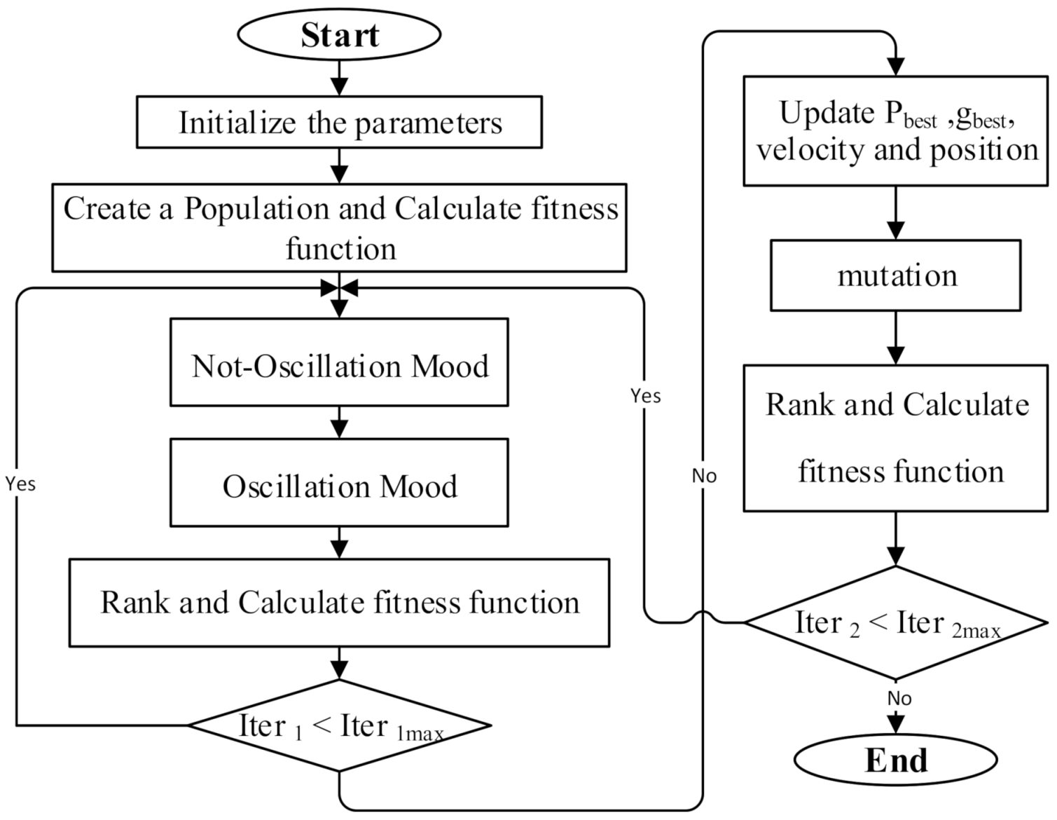
3. The Proposed Method

3.1. Hybridizing AIWPSO with EMA

In this study, the combination of EMA and AIWPSO algorithms was suggested for solving the CEED problem. In this section, how to combine these two algorithms to solve constrained CEED problems, and incorporating a constraint handling technique, is described. Figure 1 shows the flowchart of the presented method. The steps of hybridizing AIWPSO with EMA based on the methods suggested by Nourianfar and Abdi [51] and Li et al. [46] are highlighted below:

Step 1. (Initialization): In the first step, the adjustable parameters are set. The optimal value of these parameters for various problems will be different, which can be obtained through various methods. In this study, constant values for the parameters are considered, and their optimal values are obtained through empirical analysis. This is an accepted method among most researchers widely used for tuning the parameters of the metaheuristic algorithms [52]. The selecting method of optimal values for g₁[max, min] and g₂[max, min] is described in [47]. The appropriate values of mu, C_1i, C_1f, C_2i, and C_2f, in most simulations are 0.5, 0.5, 2.5, 0.5, and 2.5, respectively.

Step 2. (Generate an initial population): The outputs power are the decision variables. Therefore, the initial generation power regarding each unit is determined using Equation (13):

$$P_a^{min}{}^{*}=Max\left(P_a^{min}, P_a^0-D{R}_a\right)$$

(11)

$$P_a^{max}{}^{*}=Min\left(P_a^{max}, P_a^0-U{R}_a\right)$$

(12)

$$P_a=P_a^{min}{}^{*}+rand\times \left(P_a^{max}{}^{*}-P_a^{min}{}^{*}\right) i=1,\dots ,N$$

(13)

in which, n is the number of population, and rand is a random number in the range of 0–1. The primary speed of all variables of each member is assumed to be equal to zero [51]. The position calculated by Equation (13) for each population was set as P_best of that population. The least P_best value was also chosen as g_best.

Step 3. (Fitness function): In this step, the fitness function (FF) for each member of the population will be calculated. The calculation of the fitness function is discussed in detail later in Section 3.2. In the following, the best fitness is selected and is known as g_best [51].

Step 4. (Not-Oscillation Mood): In this step, the population is ranked according to the fitness function and is divided into three different groups. The number of the population in each group is specified. The first group stays intact and unchanged, which is usually 20% of the population. The second group includes usually 30% of the population and is changed as follows [47]:

$$PO{P}_j^{group2}=\alpha \times PO{P}_{1,i}^{group1}+\left(1-\alpha \right)\times PO{P}_{2,i}^{group1} i=1,2,\dots ,N,j=1,2,\dots ,M$$

(14)

in which, n is the number of first group members, and M is the number of second group members. $\alpha$ is an accident number in the range [0,1]; $PO{P}_{1,i}^{group1}$ and $PO{P}_{2,i}^{group1}$ are the members of the group 1; and $PO{P}_j^{group2}$ is the jth member of group 2.

The number of the population in group 3 is usually selected to be equal to half of the total members, and they make the worst population according to the fitness function [51]. The members of this group are changed according to the following equation [47]:

$${\delta }_k=2\times r_1\times \left(PO{P}_{i,1}^{group1}-PO{P}_k^{group3}\right)+2\times r_2\times \left(PO{P}_{i,2}^{group1}-PO{P}_k^{group3}\right)$$

(15)

$$PO{P}_k^{group3,new}=PO{P}_k^{group3}+0.8\times {\delta }_k k=1,2,\dots ,N_k$$

(16)

in which $r_1$ and $r_2$ are assumed to be two numbers that are randomly selected in the range 0 to 1. $N_k$ is the Nth member of the third group. $PO{P}_k^{group3}$ is the kth member in group 3, and ${\delta }_k$ is the change value of the kth member in the third group, based on the difference between that member and the two members of the first group.

Step 5. (Oscillation Mood): The population is ranked and subdivided into three groups, in this step, as follows: The first group stays fixed. In the second group, the number of the relevant variables increased as follows [47]:

$$\Delta n_{t1}=n_{t1}-\theta +\left(2\times r\times \mu \times {\omega }_2\right)$$

(17)

$$\mu =\left(\frac{t_{POP}}{n_{POP}}\right)$$

(18)

$$n{t}_1={\displaystyle \sum }_{y=1}^n\left|S_{ty}\right|$$

(19)

$${\omega }_2=n{t}_1\times g_1^k$$

(20)

$$g_1^k=g_{1,max}-\frac{g_{1,max}-g_{1,min}}{ite{r}_{1max}}\times k$$

(21)

where $\Delta n_{t1}$ is the increment value that is added to a number of variables. $n{t}_1$ is the value that is calculated from the sum of all the variables of member t before implementing the changes, and $S_{ty}$ is the variable yth according to member t. $\theta$ is a given value based on the problem, which is $n{t}_1$, in the case that no penalty factor is used (e.g., for the ELD problem without considering losses equals P_D). r is an accident number in the range of [0,1], and ${\omega }_2$ is the level of risk associated with all members in group 2. Additionally, $t_{POP}$ and $n_{POP}$ are the indexes for the current population and the last population in the algorithm procedure, respectively. μ is a constant parameter regarding each member, and $g_1^k$ is also an ordinary level risk in kth iteration, which decreases by increasing the iteration number. $ite{r}_{max}$ is the maximum iterations of the EMA loop, and k is the index of iteration. $g_{1,min}$ and $g_{1,max}$ are also the lowest and highest level of relevant risk, respectively.

After the above process, each member of the population whose sum of variables has been increased by $\Delta n_{t1}$ must change the value of its variables in such a way that the sum of the variables reduces by the same amount [51]. Therefore $\Delta n_{t2}$, the decrement amount, is calculated as follows:

$$\Delta n_{t2}=n_{t2}-\theta$$

(22)

where $\Delta n_{t2}$ is the value that must be subtracted from the sum of the member variables that have already been incremented, and $n_{t2}$ is the total variables of the tth member. For members in group 3, the $\Delta n_{t3}$ value is calculated as follows [47]:

$$\Delta n_{t3}=\left(4\times r_s\times \mu \times {\omega }_3\right)$$

(23)

$$r_s=\left(0.5-rand\right)$$

(24)

$${\omega }_3=n{t}_1\times g_2^k$$

(25)

$$g_2^k=g_{2,max}-\frac{g_{2,max}-g_{2,min}}{ite{r}_{1max}}\times k$$

(26)

in which $\Delta n_{t3 }$ is a value that is randomly added or subtracted from the variables of members in this group. $r_s$ is a random number, and ${\omega }_3$ is the level of risk associated to the third group. μ is a coefficient that increases members’ risk.

Step 6. (Ranking and recalculating the fitness function): In this step, the fitness function is recalculated for all members of the population and ranked accordingly (the best member has the lowest total cost). If the new values of P_best for each member are better than the previous ones, new values are replaced with the previous values. The best value among these P_best is selected as g_best, if it is better than previous ones.

Step 7. (Checking the maximum iteration for EMA loop): In this step, if the maximum iteration of the EMA loop is reached, it will break; otherwise, steps 4–7 will be repeated, again.

Step 8. (Updating the velocity, position, P_best, and g_best.): At the beginning of this step, P_best and g_best of each member of the population are updated based on the comparison of the value of their current fitness function and their initial value P_best and g_best. Then, the position and velocity of the population are updated as follows:

$$V_{i,j}^{it+1}=w^{it}\times V_{i,j}^{it}+C_1^{it}\times r_1\times \left(P_{best,j}-PO{P}_{i,j}^{it}\right)+C_2^{it}\times r_2\times \left(g_{best,j}-PO{P}_{i,j}^{it}\right)$$

(27)

$$PO{S}_{i,j}^{it+1}=PO{S}_{i,j}^{it}+\frac{2}{2-\psi -\sqrt{{\psi }^2-4\psi }}\times V_{i,j}^{it+1}$$

(28)

$$C_1^{it}=C_{1i}+\frac{C_{1f}-C_{1i}}{ite{r}_{2max}}\times it$$

(29)

$$C_2^{it}=C_{2i}+\frac{C_{2f}-C_{2i}}{ite{r}_{2max}}\times it$$

(30)

$$\psi =C_1^{it}+C_2^{it}$$

(31)

where it represents the number of iteration; $i{t}_{max}$ is the maximum iteration number; and $V_{i,j}^{it+1}$ and $PO{S}_{i,j}^{it+1}$ are the speed and position of variable j regarding population i at the iteration it + 1, respectively. $C_1^{it}$ and $C_2^{it}$ are acceleration coefficients at the iteration it, and subscripts i and f represent their initial and final values. Furthermore, in order to improve the balance between the global exploration and local exploitation, the value of $w^{it}$ is calculated as follows [46]:

$$w^{it}=0.5rand+\frac{fitnes{s}_{g_{best}}^{it}}{fitnes{s}_{P_{best,j}}^{it}}$$

(32)

where $fitnes{s}_{g_{best}}^{it}$ shows the fitness of g_best at the iteration it, and $fitnes{s}_{P_{best,i}}^{it}$ is the fitness of P_best for the jth variable. More details on the procedure of the adaptive inertia weight equation and AIWPSO algorithm are given by Li et al. [46].

Step 9. (Mutation): To increase the chances of finding the optimum solution and expand search space, the mutation operator was used. The value of the change in the variable i of the population j in each mutation was obtained according to the following equation:

$${\Delta }_{i,j}=pm\times \left(X_{i,j}^{max}-X_{i,j}^{min}\right)$$

(33)

$$pm={(1-\frac{\left(it-1\right)}{\left(i{t}_{max}-1\right)})}^{\raisebox{1ex}{$5$}\!\left/ \!\raisebox{-1ex}{$mu$}\right.}$$

(34)

where ${\Delta }_{i,j}$ is the changes related to the jth variable of member I; $X_{i,j}^{min}$ and $X_{i,j}^{max}$ are the minimum and maximum range of the jth variable of member I, respectively; and mu is the mutation rate.

Step 10. (Ranking and recalculating the fitness function): In this step, the fitness function is recalculated for all members of the population and ranked accordingly. Then, P_best and g_best of each member of the population are updated, if needed.

Step 11. (Checking the maximum iteration for the termination of hybrid algorithm): In this step, the maximum iteration is checked. If the stopping criterion is achieved, the procedure ends. Otherwise, the algorithm returns to step 4.

3.2. Constraint Handling

In this study, the MCR Technique was used to handle the constraints of the problem [48]. The MCR was designed to overcome the handling of constraints with different orders of magnitude or different units. This technique assigns a separate violation rank for each constraint. The MCR is not embedded into the optimization algorithm and is in fact an uncoupled approach. This feature allows it to be implemented along with different evolutionary algorithms [48].

First, we defined each of the equality constraints as an inequality one as follows:

$$h_j\left(\overrightarrow{x}\right)=0 \to \left| h_j\left(\overrightarrow{x}\right)\right|-\delta \le 0$$

(35)

in which δ is a small-enough positive value, and $h_j\left(\overrightarrow{x}\right)$ is the jth equality constraint. Therefore, any constraint violation j of the candidate solution $\overrightarrow{x}$ is calculated as follows:

$$v_j\left(\overrightarrow{x}\right)=max\left\{0, \left|h_j\left(\overrightarrow{x}\right)\right|-\delta \right\}$$

(36)

where $v_j\left(\overrightarrow{x}\right)$ is the violation value of the jth constraint. Then, the fitness function regarding each member of the population is obtained using Equation (37) [48].

$$FF=\left\{\begin{array}{c}{R}_{Nv}+{\displaystyle {\displaystyle \sum }_{i=1}^m}{R}_{\phi }^j \mathrm{if} \mathrm{only} \mathrm{infeasible} \mathrm{individuals} \\ R_f+R_{Nv}+{\displaystyle {\displaystyle \sum }_{i=1}^m}{R}_{\phi }^j \mathrm{otherwise} \end{array} \right.$$

(37)

in which, $R_f$, $R_{Nv}$, and $R_{\phi }^j$, the calculated ranks are according to the objective value, the number of violated constraints, and the violation value of jth constraint.

As can be seen from Equation (37), the fitness function, in addition to ranking the violation value of each constraint, also depends on the rank of the number of violated constraints of each solution. This means that a solution with a greater number of violated constraints but lower values of the violation is not superior to a solution with a dominant constraint violation (the value of the violation with a high order of magnitude). Thus, if there are two constraints with different orders of magnitude in an optimization problem, both will have the same effect on the fitness function. In addition, as can be seen in Equation (37), the ranking of the objective function is performed only if there is at least one feasible solution. This means that when all the solutions are infeasible, the calculations related to the ranking of the objective function are not performed, and consequently less time is spent. Therefore, in the CEED problem, the power balance constraint becomes inequality ones, and then the fitness function for each member of the population is calculated according to (37). The advantage of this technique is that it does not need any user-predefined parameter setting, and it follows a relatively simple logic, which makes it easy to implement [48].

4. Simulation Case Study Results

To illustrate the effectiveness and ability of the presented method, it was applied to six benchmark functions and five CEED test systems including 6, 30 (IEEE (Institute of Electrical and Electronics Engineers) standard case), 10, 40 (Taiwan test system), and 14 units test systems. The test systems were arranged from simple to more complex cases. Additionally, to prove the superiority of the suggested method, the obtained results were compared with other optimization methods in this field. The proposed algorithm parameter settings are shown in

Table 1. Parameter settings.

Parameter	Case Study Number
	1	2	3	4	5
Population	50	50	100	100	200
C1i, C2i	0.5	0.5	0.5	0.46	0.52
C1f, C2f	2.5	2.5	2.5	1.96	2.5
g1 [max, min]	[0.02, 0.002]	[0.05, 0.04]	[0.02, 0.002]	[0.02, 0.002]	[0.02, 0.002]
g2 [max, min]	[0.01, 0.001]	[0.04, 0.03]	[0.01, 0.001]	[0.01, 0.001]	[0.01, 0.001]
Max-iteration of EMA loop	50	50	50	50	50
Max-iteration	10	10	10	10	10
mu	0.5	0.5	0.5	0.4	0.4
PPF	62.036	65.216	43.559	1.8343	1.2189 1

¹ PPF For 2150 MW is 1.5299 and for 2650 MW is 1.5715.

. In addition, to extract Pareto-optimal solutions, first by using the PPF, the CEED problem was converted into a single-objective problem, and then by changing the φ values from 0 to 1, with an incremental rate of 0.025, different Pareto solutions were obtained. All simulations were performed under the MATLAB (Matrix Laboratory) environmental and were implemented on a laptop with CPU (Central Processing Unit) 1.5 GHz and RAM (Random Access Memory) 8 GB.

4.1. Benchmark Functions

To evaluate the performance of the algorithm, six benchmark functions were applied. The data of these functions are presented in [46]. The statistical results of the proposed method compared to CPSO, APSO, and AIWPSO for the 30 independent trials and with 30 dimensions are shown in

Table 2. Comparisons of the statistical results of the different methods for benchmark functions.

Function Name		CPSO [46]	APSO [46]	AIWPSO [46]	Proposed Method
Sphere	Mean	4.24 × 10−4	4.73 × 10−4	7.14 × 10−15	3.22 × 10−55
	Min	2.12 × 10−4	2.55 × 10−4	2.59 × 10−15	1.41 × 10−55
Rosenbrock	Mean	2.94 × 101	2.82 × 101	2.18 × 101	2.24 × 10−8
	Min	2.26 × 101	2.22 × 101	1.99 × 101	1.89 × 10−8
Ackley	Mean	5.60 × 101	2.51 × 101	1.72 × 10−4	8.08 × 10−19
	Min	1.70 × 101	1.12 × 101	8.70 × 10−10	3.77 × 10−20
Rastrigin	Mean	2.34 × 102	1.25 × 101	2.40 × 10−14	1.90 × 10−38
	Min	1.24 × 102	1.03 × 100	1.24 × 10−14	1.54 × 10−40
schwefel P2.22	Mean	4.11 × 10−1	3.15 × 10−1	4.20 × 10−2	6.20 × 10−15
	Min	2.05 × 10−1	1.15 × 10−1	1.09 × 10−2	1.15 × 10−15
Rotated hyper ellipsoid	Mean	1.34 × 101	1.32 × 101	2.62 × 10−14	2.44 × 10−23
	Min	6.10 × 10−2	4.52 × 10−2	1.01 × 10−14	2.32 × 10−25

.

Benchmark functions are employed to evaluate different aspects of algorithm performance. For example, due to the unimodal nature of the Sphere function, its results can be used to investigate the convergence rate of the algorithm. In addition, since Rosenbrock, Ackley, and Rastrigin functions are typical multimodal functions, the results of applying the algorithms to these functions can be used to evaluate the algorithm ability in finding the global optimum.

Table 2 shows that the min value of the results obtained by applying the proposed method is lower than the other methods in all six benchmark functions, which demonstrates high ability of the suggested algorithm to find a global optimum. Additionally, the low deviation between the mean value of the obtained results by the proposed method and the minimum value confirms the proposed method robustness.

4.2. Case Study 1

In this case study, a simple test system with six units was used. The details of this system are taken from [53] where the power demand was 1200 MW. The simulation results for the proposed method were compared with the other algorithms and are detailed in

Table 3. Comparison of the results of different techniques for different methods.

Output	P1 (MW)	P2 (MW)	P3 (MW)	P4 (MW)	P5 (MW)	P6 (MW)	Cost ($/h)	Emission (lb/h)	Total Power (MW)	Power Losses (MW)
QTLBO [54]	107.310	121.497	206.501	206.583	304.984	304.604	64912	1281	1251.478	51.478
BBTLBO 1 [54]	56.826	74.003	197.791	224.262	321.621	325.000	60863	1294.7	1199.502	50.109
MODE [54]	108.628	115.946	206.797	210.000	301.888	308.413	64843	1286	1251.672	NA 2
Proposed Method	107.150	119.848	206.172	206.227	307.080	304.435	64841	1281	1250.912	50.912

¹ Power balance is not met. ² Not available.

.

The above table depicts that the obtained results by applying the presented method are better than the other techniques. For example, the annual cost savings resulting from applying the proposed method compared to QTLBO [54] and MODE [54] were equal to USD 621,960 and 17,520, respectively. Moreover, the power losses obtained by the proposed method were less than the other methods. It should be noted that the solution of the BBTLBO [54] is infeasible because the power balance constraint has been violated. As can be seen, in this case, due to the low complexity and small scale of the test system, the results are close to each other. Hence, this issue can be used to compare the local exploitation ability of methods.

4.3. Case Study 2

In this case study, the VPLE was modeled. The values are given in p.u on a 100 MVA base. The emission and cost coefficients are presented in [55]. The results are compared with other methods and are tabulated in

Table 4. Comparison of minimum fuel and emission, and best compromise solution for case study 2.

Methods		Cost ($/h)	Emission (ton/h)	Losses (p.u)		Cost ($/h)	Emission (ton/h)	Losses (p.u)
WGSO [15]	φ = 1	613.469	0.22331	NA	φ = 0	679.318	0.19418	NA
GSO-T [12]		613.463	0.22343	NA		679.221	0.19418	NA
KKO [56]		605.68	0.21789	0.023		646.457	0.19418	0.034
ISA [12]		613.274	0.22265	NA		659.365	0.19356	NA
KSO [57]		605.896	0.2211	0.025		646.600	0.1942	0.035
Proposed Method		612.913	0.200 57	0.028		677.432	0.18607	0.030

. The generated output powers are presented in

Table A1. The generated output powers for case study 2.

Methods		P1 (p.u)	P2 (p.u)	P3 (p.u)	P4 (p.u)	P5 (p.u)	P6 (p.u)
φ = 1	WGSO [15]	0.56521	0.40004	0.68748	0.95051	0.55006	0.2238
	GSO-T [12]	0.51661	0.40127	0.6876	0.95063	0.55008	0.22721
	KKO [56]	0.1295	0.3224	0.5419	0.9690	0.5295	0.3654
	ISA [12]	0.0533	0.3956	0.6751	0.9354	0.5365	0.22967
	KSO [57]	0.1127	0.2917	0.5811	0.9953	0.5261	0.3524
	Proposed Method	0.05017	0.38415	0.6875	0.8	0.54999	0.39
φ = 0	WGSO [15]	0.41071	0.46396	0.54358	0.39035	0.54366	0.51461
	GSO-T [12]	0.40982	0.46383	0.54414	0.38954	0.54461	0.5149
	KKO [56]	0.4128	0.4617	0.5455	0.3867	0.5457	0.5162
	ISA [12]	0.36474	0.38945	0.49354	0.53432	0.57284	0.48465
	KSO [57]	0.4111	0.4624	0.5436	0.3909	0.5479	0.5156
	Proposed Method	0.39467	0.4972	0.50726	0.45938	0.50793	0.49749

, in Appendix A. The pareto-front obtained by the proposed method is plotted in Figure 2. This figure shows that the proposed method can extract the Pareto optimal solutions with proper distribution and uniformity.

Table 4 depicts that the proposed method is superior to the other methods in obtaining the lowest emission for φ = 0. Nonetheless, for φ = 1, the least cost obtained is related to the KKO algorithm, which indicates its superiority in finding the least cost. In these cases, according to the concept of domination and considering both objectives, it is not possible to determine which of these methods is superior to the other. To illustrate the robustness and reliability of the suggested method, the maximum, minimum, average, and standard deviation of the cost obtained for 100 trial runs were compared with the other reported methods and are depicted in

Table 5. Comparison of min, max, mean, and Std. obtained from 100 trial runs of various techniques.

Method	Cost ($/h)			Std.
	Min	Max	Mean
WGSO [15]	613.4694	614.5266	613.6621	0.0031082
GSO-T [12]	613.4626	613.9756	613.6830	0.0016427
ISA [12]	613.274	613.952	613.398	0.001035
Proposed method	612.913	613.325	613.024	0.000937

.

It is seen that the mean value of the cost obtained by the presented method is very close to its minimum value. This fact indicates that the presented method has excellent exploration characteristic in the solution space.

4.4. Case Study 3

In this case, the suggested method is applied to a ten units’ system. In this case, the VPLE and the transmission line losses are modeled. The details of this system are given in [12]. Power outputs, emission, CPU time, and cost obtained from algorithms of KKO [56], KSO [57], ISA [12], GWO-AWDO [58], GSA [59], CIHSA [32], and the proposed method are presented in

Table 6. Comparison of the BCS obtained from different methods for system test 3.

Output	KKO	GSA	KSO	ISA	GWO-AWDO	CIHSA	Proposed Method
							Emission	Cost
P1	54.992	54.999	55.000	53.143	54.944	55.00	55.00	55.00
P2	78.891	79.958	80.000	78.965	79.730	80.00	80.00	80.00
P3	78.794	79.434	81.134	78.103	80.133	81.081	81.134	89.016
P4	88.747	85.000	81.3637	97.117	86.226	80.93	81.363	85.755
P5	159.814	142.106	160.000	152.74	143.590	160.0	160.0	102.92
P6	160.555	166.567	240.000	163.02	165.942	240.0	240.0	112.63
P7	262.174	292.874	294.485	257.94	292.770	290.8	294.48	300.0
P8	308.857	313.238	297.270	302.14	312.457	296.689	297.27	326.78
P9	430.307	441.177	396.765	432.76	440.304	398.842	396.76	464.44
P10	461.039	428.630	395.576	465.86	427.815	398.331	395.57	470.0
Cost ×105 ($/h)	1.13481 *	1.1349	1.16412	1.1217 *	1.1330 *	1.1639	1.16411	1.1180
Emission (ton/h)	3982.85 *	4111.4	3932.24	3995.6 *	4108.80	3932.44	3932.20	4384.3
CPU (s)	NA	NA	NA	2.04	NA	NA	2.31	2.27
Losses (MW)	84.17	83.98	81.59	NA	83.91	81.67	81.6	86.5

* invalid.

. The pareto-front extracted by the proposed method is depicted in Figure 3.

This case, due to the increasing size of the problem and considering the practical constraints, as well as the emission as one of the objectives, can be mentioned as a good benchmark for evaluating the algorithm performance in solving the CEED problems.

As can be seen from Table 6, the minimum solution cost obtained by the proposed method is the lowest cost among the other methods. Additionally, the minimum emission solution obtained by the proposed method dominates the solution obtained by KSO.

Since in other cases, either the cost is lower and the emission is higher or vice versa, it is not possible to certainly determine which method is superior. To fairly compare the proposed method with GSA, GWO-AWDO, KKO, and ISA, in Figure 3, the other two solutions obtained by the proposed method (shown by the letters “B” and “C”) were compared with the solution obtained by them (shown by their acronyms). It should be noted that the correct cost of the GWO-AWDO is 1.1352 × 10⁵. In addition, the outputs of KKO and ISA are invalid, and their correct costs and emissions are 1.1376 × 10⁵, 4115.5, and 1.1352 × 10⁵, 4138.3. Similarly, to compare with the CIHSA, another solution of the proposed method (shown by the letter “A”) is compared with the solution obtained by the CIHSA in Figure 3.

By comparing the results, it can be seen that solution (B) obtained by the proposed method dominates the solutions obtained by the three methods of GSA, GWO-AWDO, and KKO. In the same way, solutions (A) and (C) dominate the solutions obtained by the CIHSA and ISA methods, respectively. This means that these solutions are less costly and lower in emissions. The amounts of fuel cost obtained for 100 trial runs are presented in Figure 4.

4.5. Case Study 4

In order to demonstrate the ability of the proposed method to solve large-scale problems, the complex test system included 40 units and was used by considering the VPLE. The fuel cost coefficients are given in [60], and the emission factors are given in [18]. The generated output powers are presented in Figure 5 and are tabulated in

Table A2. The generated output powers for case study 4.

	KSO	NSGA-II	MGAIPSO	GWO-AWDO	KKO	APSO	CIHSA	AWDO	Proposed Method
P1	112.80	113.868	111.056	113.542	114.00	114	114	113.703	113.999
P2	112.68	113.638	110.770	114.023	113.045	114	114	114	114
P3	119.67	120	97.397	119.808	119.744	120	120	119.936	119.999
P4	179.66	180.788	129.866	181.147	181.102	178.711	169.368	180.531	171.912
P5	96.68	97	87.799	97.940	96.5081	97	97	97	97
P6	139.72	140	105.411	139.204	139.796	129.8	124.257	138.312	124.221
P7	298.30	300	259.584	300.439	299.686	300	299.711	300	299.506
P8	284.60	299.008	209.799	299.347	298.619	299.700	297.914	300	300
P9	284.60	288.889	284.500	296.159	289.447	298.8	297.260	297.139	300
P10	130.00	131.613	130.001	130.244	131.386	130	130	130.919	136.077
P11	311.49	246.512	318.367	245.322	247.114	308.2	307.573	245.219	292.776
P12	315.59	318.874	318.416	318.268	318.381	307.6	307.001	318.063	292.294
P13	394.28	395.722	394.277	393.914	395.689	433.981	433.807	394.237	423.689
P14	394.28	394.136	394.278	396.696	393.82	407.5	408.955	396.475	405.035
P15	394.28	305.578	394.276	307.591	305.891	410	411.450	306.860	406.808
P16	394.28	394.696	394.279	393.400	394.283	410	411.450	393.945	406.808
P17	488.33	489.423	399.519	489.380	489.706	453.314	452.156	489.859	440.447
P18	497.57	488.270	399.519	487.768	487.897	453.400	452.179	488.569	440.451
P19	487.59	500.8	508.151	497.993	500.104	437.300	437.466	497.988	444.520
P20	421.52	455.200	50.863	455.443	455.719	437.311	437.466	454.853	444.520
P21	433.54	434.663	515.033	432.103	434.334	437.403	437.467	432.555	446.889
P22	433.54	434.15	517.355	434.788	434.86	437.381	437.467	434.265	446.890
P23	433.62	445.838	516.261	444.529	446.6	437.873	437.976	444.707	447.2
P24	433.57	450.750	433.521	452.917	451	437.934	437.976	452.868	447.2
P25	433.52	491.274	510.139	493.187	491.259	437.6	437.759	492.267	447.25
P26	433.52	436.341	512.540	434.464	435.771	437.600	437.759	434.136	447.25
P27	10.00	11.245	10.000	11.641	11.079	19.143	19.531	10.753	23.7527
P28	10.00	10	10.001	10.248	10.3466	19.148	19.531	11.108	23.753
P29	10.00	12.071	10.003	11.935	12.2337	19.140	19.531	11.191	23.7527
P30	97.00	97	87.786	96.064	96.6001	97	97	97	97
P31	187.91	189.482	159.747	188.447	189.436	176.100	175.807	189.252	175.035
P32	186.12	174.797	159.734	174.844	175.188	176.1	175.807	174.634	175.035
P33	188.51	189.284	159.738	188.497	189.992	176.1	175.807	188.809	175.035
P34	199.72	200	199.992	199.587	199.679	200	200	200	200
P35	200.00	199.913	199.998	199.195	199.89	200	200	198.656	200
P36	200.00	199.503	164.801	200.008	199.905	200	200	200.456	200
P37	110.00	108.306	89.112	109.591	108.554	104.5	104.255	109.428	101.789
P38	110.00	110	89.116	109.871	109.71	104.5	104.255	110	101.790
P39	110.00	109.789	89.112	108.041	108.639	104.5	104.255	108.507	101.790
P40	421.52	421.560	58.868	422.395	421.912	437.356	437.466	421.782	444.521

in Appendix A. In addition, the emissions and the cost obtained by the suggested method and the other reported methods are presented in Figure 6.

Figure 6 shows that, compared with the KSO, NSGA-II, MGAIPSO, GWO-AWDO, KKO, ISA, APSO, CIHSA, and AWDO algorithms, the cost was reduced by $/h 3693, $/h 4033, $/h 2863, $/h 1373, $/h 4053, $/h 1233, $/h 6823, $/h 6923, and $/h 1423, respectively; while the emissions were reduced by 21520 ton/h, 32880 ton/h, 23570 ton/h, 32030 ton/h, 32760 ton/h, 28360 ton/h, 800 ton/h, 500 ton/h, and 32230 ton/h, respectively. As can be seen, by increasing the test system size, the suggested method performance improves. This means that the suggested method is more favorable to large-scale systems. Since, in practice, the power systems are large-scale, the proposed method can be considered as an effective candidate to optimize the EED problems in real power systems.

4.6. Case Study 5

To evaluate the performance of the suggested method in solving a constrained CEED problem, it is implemented on a test system including 14 thermal generating units. In this case, the RRLs, the transmission electrical losses, the VPLE, and POZs are mentioned as a package. The data of the 14-unit system are derived from [61] and are represented in Appendix B. The power outputs obtained by applying the proposed method for three load demands of 1750, 2150, and 2650 MW in ELD, emission-constrained dispatch (ECD), and CEED are shown in

Table 7. The outputs found by the proposed method for load demands of 1750, 2150, and 2650 MW.

Output	1750 MW			2150 MW			2650 MW
	ECD	ELD	CEED	ECD	ELD	CEED	ECD	ELD	CEED
P1	280.000	329.5235	280.024	284.523	419.280	329.519	388.041	419.281	419.279
P2	180.000	225.000	180.016	180.021	299.611	185.000	225.000	374.402	225.000
P3	79.892	20.000	94.799	129.992	94.800	105.721	129.991	111.719	129.989
P4	90.965	69.802	69.8665	119.730	119.733	119.733	129.990	119.732	129.972
P5	150.000	150.000	150.011	150.034	150.012	150.026	170.000	169.800	169.984
P6	280.000	280.000	284.599	334.470	284.600	284.600	460.000	420.000	455.000
P7	230.000	233.857	234.733	234.730	234.730	234.733	410.491	334.468	384.332
P8	73.005	60.000	60.022	159.730	60.007	159.733	159.987	159.731	159.733
P9	74.425	74.8621	74.8665	159.998	124.731	159.992	159.993	124.729	162.000
P10	91.175	137.183	99.800	159.999	137.201	159.991	159.991	159.995	159.992
P11	44.366	56.784	57.400	79.991	57.400	79.991	79.987	79.991	79.993
P12	73.005	54.000	64.383	55.000	79.285	79.993	79.992	79.991	79.994
P13	73.282	62.362	62.400	84.992	62.400	84.992	84.988	84.989	84.993
P14	45.820	15.000	52.400	54.889	52.400	52.400	54.989	52.400	54.968
Cost ($/h)	9514.64	8325.21	8750.39	11,279.83	10,149.54	10,746.22	15,040.11	13,961.90	14,514.16
Emission (lb/h)	2984.36	3940.82	3047.57	4046.56	6159.26	4180.65	7865.89	9528.07	7918.40
Losses (MW)	15.93	18.37	15.32	38.09	26.19	36.42	43.44	41.22	45.22

.

The emission, cost, and total cost (TC) of the suggested method in ECD, ELD, and CEED for different load cases were compared with the methods of APSO [62] and SOHPSO-TVAC [61] in

Table 8. Comparison of the result obtained by ECD, ELD, and CEED.

Method			APSO [62]	SOHPSO-TVAC [61]	Proposed Method
Load (MW)	1750	ECD (Emission) (lb/h)	2984.431	3182.50	2984.36
		ELD (Cost) ($/h)	8322.003	8621.52	8325.21
		CEED (Total Cost) ($/h)	12,491.322	12,745.692	12,465.08
	2150	ECD (Emission) (lb/h)	4075.5318	4603.90	4046.56
		ELD (Cost) ($/h)	10,222.371	10,778.00	10,149.54
		CEED (Total Cost) ($/h)	17,159.145	18,876.501	17,142.20
	2650	ECD (Emission) (lb/h)	7877.248	8269.90	7865.89
		ELD (Cost) ($/h)	14,080.275	14,209.00	13,961.90
		CEED (Total Cost) ($/h)	26,963.048	30,382.425	26,957.93

. Table 7 shows that all constraints were met. For all levels of power demand and in all three problems of ELD, ECD, and CEED, based on the prohibited operating zones shown in

Table A4. POZs for 14-unit system.

Unit	POZs
2	[185 225] [305 335] [420 450]
5	[180 200] [305 335] [390 420]
6	[230 255] [36 395] [430 455]
12	[30 40] [55 65]

in the Appendix B, it can be seen that the generated power outputs of units 2, 5, 6, and 12 do not violate the relevant prohibited zones. In addition, none of the ramp rate limits of units were violated according to

Table A5. RRLs for 14-unit system.

Unit	${\mathit{P}}_{\mathit{a}}^0$	$\mathit{D}{\mathit{R}}_{\mathit{a}}$	$\mathit{U}{\mathit{R}}_{\mathit{a}}$
1	400	120	80
2	300	120	80
3	105	130	130
4	100	130	130
5	90	120	80
6	400	120	80
7	350	120	80
8	95	100	65
9	105	100	60
10	110	100	60
11	60	80	80
12	40	80	80
13	30	80	80
14	20	55	55

, and the power balance constraint was met with good accuracy. For example, the location of the power outputs of units 2 among its prohibited operating zones is shown in Figure 7, for all levels of power demand and in all three problems of ELD, ECD, and CEED. As can be seen from this figure, none of the power outputs are in prohibited zones. Therefore, it can result that the suggested technique is suitable for dealing with constrained optimization problem. Additionally, its constraints handling capability was verified.

The best results are bold in Table 8 for each item. As seen in Table 8, the proposed method in eight items has the best solution and performs only in one item weaker than the APSO algorithm. Therefore, the proposed method is capable of solving CEED problems containing operational constraints, while it also has the best performance among other methods.

4.7. Discussion

4.7.1. Computation Time

The computation time is directly proportional to the CPU speed. Hence, in this study, in addition to absolute run time, the relative run time was also used to assess the computational complexity of different algorithms. The relative run time was obtained from the following equation [3]:

$$RR{T}_{i,j}=AR{T}_i\times \frac{CPUSpee{d}_i}{CPUSpee{d}_j}$$

(38)

Table 9. The absolute and relative run times for different test systems.

Case Study Number		CPU Speed (GHz)	ART	RRT
1	TLBO	2	2.18	2.90
	QTLBO	2	1.91	2.54
	BBTLBO 1	NA	NA	NC 1
	MODE	3	3.09	6.18
	Proposed method	1.5	2.01	2.01
2	ISA	NA	2	NC
	KSO	2.4	NA	NC
	Proposed method	1.5	2.02	2.02
3	GWO-AWDO	2.2	NA	NC
	ISA	NA	2.04	NC
	CIHSA	3.5	NA	NC
	PDE	3	4.23	8.46
	SPEA-2	3	7.53	15.06
	KSO	2.4	NA	NC
	Proposed method	1.5	2.31	2.31
4	MGAIPSO	2.5	NA	NC
	GWO/AWDO	2.2	NA	NC
	APSO	NA	NA	NC
	ISA	NA	2.72	NC
	CIHSA	3.5	NA	NC
	Proposed method	1.5	2.95	2.95
5	APSO	NA	NA	NC
	Proposed method	1.5	2.19	2.19

¹ Not calculated.

shows the comparison between the relative run time for different test systems. Table 9 shows that the proposed method is significantly faster than the other methods.

4.7.2. Convergence Characteristics

In order to check the convergence behavior of the proposed method, the convergence curves obtained by the proposed method for the study cases of 1 to 5 are shown in Figure 8. This figure shows that although the proposed method quickly reaches close to the optimal solution, the number of iterations to find the final optimal solution was relatively large. The reason is that the proposed method works in a combined manner. That is, first, using the EMA algorithm, it reaches the vicinity of the optimal solution very quickly, and then, the AIWPSO searches for a final optimal solution among the local optimal ones in the vicinity. This process may be repeated several times per each run, depending on the initial settings. However, given the above, the convergence characteristic of the proposed hybrid algorithm is acceptable and appropriate. In addition, as can be seen, the more complex the problem, the more iterations are needed to achieve the optimal solution.

5. Conclusions

In this study, a new hybrid algorithm for solving the CEED problem was proposed. The suggested method was implemented on six standard benchmark functions and five CEED test systems. Comparison of the benchmark functions results’ verified better convergence of the algorithm than the other addressed methods. In five CEED test systems, the capabilities of local exploitation, global exploration, extraction of Pareto optimal solutions, solving large-scale problems, and problems with real constraints and real-world conditions were examined, respectively. In all cases, the simulation results confirmed that the suggested technique has an excellent performance in solving CEED (especially large-scale power system) problems. Additionally, the mean, minimum, and maximum results of 100 runs showed that this method was robustness in solving the CEED problem. Moreover, in the last case study, applying the proposed method to the test system demonstrated that it can find an optimal solution, satisfying all constraints. This means that the proposed constraint handling technique works well. In addition, the comparison of run-times and convergence diagrams of the proposed method by other techniques proved that despite the hybrid nature of the algorithm; its run-time and convergence speed were reasonable and acceptable. Solving the test systems in an uncertain framework including CHP units, renewable energy sources, market conditions, and electric vehicles, and taking into account more practical constraints of the system, such as multi-fuel, steady-state security conditions, and line flow limits can be considered as the priorities in future works.

References

1. Bora, T.C.; Mariani, V.C.; dos Santos Coelho, L. Multi-objective optimization of the environmental-economic dispatch with reinforcement learning based on non-dominated sorting genetic algorithm. Appl. Therm. Eng. 2019, 146, 688–700. [Google Scholar] [CrossRef]
2. Rex, C.E.; Beno, M.M.; Annrose, J. A solution for combined economic and emission dispatch problem using hybrid optimization techniques. J. Electr. Eng. Technol. 2019, 1–10. [Google Scholar] [CrossRef]
3. Murugan, R.; Mohan, M.R.; Rajan, C.C.; Sundari, P.D.; Arunachalam, S. Hybridizing bat algorithm with artificial bee colony for combined heat and power economic dispatch. Appl. Soft Comput. 2018, 72, 189–217. [Google Scholar] [CrossRef]
4. Sun, J.; Li, Y. Social cognitive optimization with tent map for combined heat and power economic dispatch. Int. Trans. Electr. Energy Syst. 2019, 29, e2660. [Google Scholar] [CrossRef] [Green Version]
5. Hajiamosha, P.; Rastgou, A.; Abdi, H.; Bahramara, S. A Piecewise Linearization Approach to Non-Convex and Non-Smooth Combined Heat and Power Economic Dispatch. J. Oper. Autom. Power Eng. 2022, 10, 40–53. [Google Scholar]
6. Hosseini-Hemati, S.; Beigvand, S.D.; Abdi, H.; Rastgou, A. Society-based Grey Wolf Optimizer for large scale Combined Heat and Power Economic Dispatch problem considering power losses. Appl. Soft Comput. 2021, 117, 108351. [Google Scholar] [CrossRef]
7. Yang, Q.; Liu, P.; Zhang, J.; Dong, N. Combined heat and power economic dispatch using an adaptive cuckoo search with differential evolution mutation. Appl. Energy 2022, 307, 118057. [Google Scholar] [CrossRef]
8. Shalini, S.P.; Lakshmi, K. Solution to Economic Emission Dispatch problem using Lagrangian relaxation method. In Proceedings of the 2014 International Conference on Green Computing Communication and Electrical Engineering (ICGCCEE), Coimbatore, India, 6 March 2014; pp. 1–6. [Google Scholar]
9. Zhan, J.P.; Wu, Q.H.; Guo, C.X.; Zhou, X.X. Fast γ-iteration method for economic dispatch with prohibited operating zones. IEEE Trans. Power Syst. 2013, 29, 990–991. [Google Scholar] [CrossRef]
10. Chen, S.D.; Chen, J.F. A direct Newton–Raphson economic emission dispatch. Int. J. Electr. Power Energy Syst. 2003, 25, 411–417. [Google Scholar] [CrossRef]
11. Bishe, H.M.; Kian, A.R.; Esfahani, M.S. A Primal-dual Interior point method for solving environmental/economic power dispatch problem. Int. Rev. Electr. Eng. 2011, 6, 1463–1473. [Google Scholar]
12. Karthik, N.; Parvathy, A.K.; Arul, R. Multi-objective economic emission dispatch using interior search algorithm. Int. Trans. Electr. Energy Syst. 2019, 29, e2683. [Google Scholar] [CrossRef] [Green Version]
13. Xiong, G.; Shuai, M.; Hu, X. Combined heat and power economic emission dispatch using improved bare-bone multi-objective particle swarm optimization. Energy 2022, 244, 123108. [Google Scholar] [CrossRef]
14. Nourianfar, H.; Abdi, H. Solving power systems optimization problems in the presence of renewable energy sources using modified exchange market algorithm. Sustain. Energy Grids Netw. 2021, 26, 100449. [Google Scholar] [CrossRef]
15. Jayakumar, D.N.; Venkatesh, P. Glowworm swarm optimization algorithm with topsis for solving multiple objective environmental economic dispatch problem. Appl. Soft Comput. 2014, 23, 375–386. [Google Scholar] [CrossRef]
16. Sakthivel, V.P.; Suman, M.; Sathya, P.D. Combined economic and emission power dispatch problems through multi-objective squirrel search algorithm. Appl. Soft Comput. 2021, 100, 106950. [Google Scholar] [CrossRef]
17. Yu, X.; Yu, X.; Lu, Y.; Sheng, J. Economic and emission dispatch using ensemble multi-objective differential evolution algorithm. Sustainability 2018, 10, 418. [Google Scholar] [CrossRef] [Green Version]
18. Shaw, B.; Mukherjee, V.; Ghoshal, S.P. A novel opposition-based gravitational search algorithm for combined economic and emission dispatch problems of power systems. Int. J. Electr. Power Energy Syst. 2012, 35, 21–33. [Google Scholar] [CrossRef]
19. Mahmoud, K.; Abdel-Nasser, M.; Mustafa, E.; M Ali, Z. Improved salp–swarm optimizer and accurate forecasting model for dynamic economic dispatch in sustainable power systems. Sustainability 2020, 12, 576. [Google Scholar] [CrossRef] [Green Version]
20. Hassan, M.H.; Houssein, E.H.; Mahdy, M.A.; Kamel, S. An improved manta ray foraging optimizer for cost-effective emission dispatch problems. Eng. Appl. Artif. Intell. 2021, 100, 104155. [Google Scholar] [CrossRef]
21. Shaheen, A.M.; El-Sehiemy, R.A.; Elattar, E.E.; Abd-Elrazek, A.S. A modified crow search optimizer for solving non-linear OPF problem with emissions. IEEE Access 2021, 9, 43107–43120. [Google Scholar] [CrossRef]
22. Elattar, E.E. Environmental economic dispatch with heat optimization in the presence of renewable energy based on modified shuffle frog leaping algorithm. Energy 2019, 171, 256–269. [Google Scholar] [CrossRef]
23. Duan, Y.; He, X. A non-convex dispatch problem with generator constraints using neural network and particle swarm optimization. Iran. J. Sci. Technol. Trans. Electr. Eng. 2020, 44, 185–196. [Google Scholar] [CrossRef]
24. Nazari-Heris, F.; Mohammadi-Ivatloo, B.; Nazarpour, D. Economic dispatch of renewable energy and CHP-based multi-zone microgrids under limitations of electrical network. Iran. J. Sci. Technol. Trans. Electr. Eng. 2020, 44, 155–168. [Google Scholar] [CrossRef]
25. Alshammari, M.E.; Ramli, M.A.; Mehedi, I.M. An elitist multi-objective particle swarm optimization algorithm for sustainable dynamic economic emission dispatch integrating wind farms. Sustainability 2020, 12, 7253. [Google Scholar] [CrossRef]
26. Sundaram, A. Multiobjective multi-verse optimization algorithm to solve combined economic, heat and power emission dispatch problems. Appl. Soft Comput. 2020, 91, 106195. [Google Scholar] [CrossRef]
27. Kansal, V.; Dhillon, J.S. Emended salp swarm algorithm for multiobjective electric power dispatch problem. Appl. Soft Comput. 2020, 90, 106172. [Google Scholar] [CrossRef]
28. Liang, H.; Liu, Y.; Li, F.; Shen, Y. A multiobjective hybrid bat algorithm for combined economic/emission dispatch. Int. J. Electr. Power Energy Syst. 2018, 101, 103–115. [Google Scholar] [CrossRef]
29. Singh, N.J.; Dhillon, J.S.; Kothari, D.P. Multiobjective thermal power load dispatch using adaptive predator–prey optimization. Appl. Soft Comput. 2018, 66, 370–383. [Google Scholar] [CrossRef]
30. Alawode, K.O.; Adegboyega, G.A.; Abimbola Muhideen, J. NSGA-II/EDA Hybrid Evolutionary Algorithm for Solving Multi-objective Economic/Emission Dispatch Problem. Electr. Power Compon. Syst. 2018, 46, 1160–1172. [Google Scholar] [CrossRef]
31. Visutarrom, T.; Chiang, T.C. Environmental/Economic Dispatch using Multiobjective Adaptive Differential Evolution with Hybrid Mutation. In Proceedings of the 2019 International Conference on Technologies and Applications of Artificial Intelligence (TAAI), Kaohsiung, Taiwan, 21 November 2019; pp. 1–6. [Google Scholar]
32. Rezaie, H.; Kazemi-Rahbar, M.H.; Vahidi, B.; Rastegar, H. Solution of combined economic and emission dispatch problem using a novel chaotic improved harmony search algorithm. J. Comput. Des. Eng. 2019, 6, 447–467. [Google Scholar] [CrossRef]
33. Yadav, N.K. Hybridization of particle swarm optimization with differential evolution for solving combined economic emission dispatch model for smart grid. J. Eng. Res. 2019, 7, 244–257. [Google Scholar]
34. Sundaram, A. Combined heat and power economic emission dispatch using hybrid NSGA II-MOPSO algorithm incorporating an effective constraint handling mechanism. IEEE Access 2020, 8, 13748–13768. [Google Scholar] [CrossRef]
35. Bhargava, G.; Yadav, N.K. Solving combined economic emission dispatch model via hybrid differential evaluation and crow search algorithm. Evol. Intell. 2020, 13, 1–9. [Google Scholar] [CrossRef]
36. Gu, H.; Zhu, H.; Chen, P.; Si, F. Improved Hybrid Biogeography-Based Algorithm for Combined Heat and Power Economic Dispatch with Feasible Operating Region and Energy Saving Potential. Electr. Power Compon. Syst. 2019, 47, 1677–1690. [Google Scholar] [CrossRef]
37. Krishnamurthy, S.; Tzoneva, R.; Apostolov, A. Method for a parallel solution of a combined economic emission dispatch problem. Electr. Power Compon. Syst. 2017, 45, 393–409. [Google Scholar] [CrossRef]
38. Man-Im, A.; Ongsakul, W.; Singh, J.G.; Boonchuay, C. Multi-objective economic dispatch considering wind power penetration using stochastic weight trade-off chaotic NSPSO. Electr. Power Compon. Syst. 2017, 45, 1525–1542. [Google Scholar] [CrossRef]
39. Mahdi, F.P.; Vasant, P.; Kallimani, V.; Watada, J.; Fai, P.Y.; Abdullah-Al-Wadud, M. A holistic review on optimization strategies for combined economic emission dispatch problem. Renew. Sustain. Energy Rev. 2018, 81, 3006–3020. [Google Scholar] [CrossRef]
40. Elattar, E.E.; Shaheen, A.M.; Elsayed, A.M.; El-Sehiemy, R.A. Optimal power flow with emerged technologies of voltage source converter stations in meshed power systems. IEEE Access 2020, 8, 166963–166979. [Google Scholar] [CrossRef]
41. Shaheen, A.M.; Elsayed, A.M.; El-Sehiemy, R.A. Optimal economic–environmental operation for AC-MTDC grids by improved crow search algorithm. IEEE Syst. J. 2021, 1–8. [Google Scholar] [CrossRef]
42. Al Harthi, M.; Ghoneim, S.; Elsayed, A.; El-Sehiemy, R.; Shaheen, A.; Ginidi, A. A Multi-Objective Marine Predator Optimizer for Optimal Techno-Economic Operation of AC/DC Grids. Stud. Inform. Control 2021, 30, 89–99. [Google Scholar] [CrossRef]
43. Elsayed, A.M.; Shaheen, A.M.; Alharthi, M.M.; Ghoneim, S.S.; El-Sehiemy, R.A. Adequate operation of hybrid AC/MT-HVDC power systems using an improved multi-objective marine predators optimizer. IEEE Access 2021, 9, 51065–51087. [Google Scholar] [CrossRef]
44. Zou, D.; Li, S.; Kong, X.; Ouyang, H.; Li, Z. Solving the combined heat and power economic dispatch problems by an improved genetic algorithm and a new constraint handling strategy. Appl. Energy 2019, 237, 646–670. [Google Scholar] [CrossRef]
45. Hsieh, M.N.; Chiang, T.C.; Fu, L.C. A hybrid constraint handling mechanism with differential evolution for constrained multiobjective optimization. In Proceedings of the 2011 IEEE Congress of Evolutionary Computation (CEC), New Orleans, LA, USA, 5 June 2011; pp. 1785–1792. [Google Scholar]
46. Li, M.; Chen, H.; Wang, X.; Zhong, N.; Lu, S. An improved particle swarm optimization algorithm with adaptive inertia weights. Int. J. Inf. Technol. Decis. Mak. 2019, 18, 833–866. [Google Scholar] [CrossRef]
47. Ghorbani, N. Combined heat and power economic dispatch using exchange market algorithm. Int. J. Electr. Power Energy Syst. 2016, 82, 58–66. [Google Scholar] [CrossRef]
48. de Paula Garcia, R.; de Lima, B.S.; de Castro Lemonge, A.C.; Jacob, B.P. A rank-based constraint handling technique for engineering design optimization problems solved by genetic algorithms. Comput. Struct. 2017, 187, 77–87. [Google Scholar] [CrossRef]
49. Nazari-Heris, M.; Mohammadi-Ivatloo, B.; Gharehpetian, G.B. A comprehensive review of heuristic optimization algorithms for optimal combined heat and power dispatch from economic and environmental perspectives. Renew. Sustain. Energy Rev. 2018, 81, 2128–2143. [Google Scholar] [CrossRef]
50. Gherbi, Y.A.; Bouzeboudja, H.; Gherbi, F.Z. The combined economic environmental dispatch using new hybrid metaheuristic. Energy 2016, 115, 468–477. [Google Scholar] [CrossRef]
51. Nourianfar, H.; Abdi, H. Solving the multi-objective economic emission dispatch problems using Fast Non-Dominated Sorting TVAC-PSO combined with EMA. Appl. Soft Comput. 2019, 85, 105770. [Google Scholar] [CrossRef]
52. Goudarzi, A.; Li, Y.; Xiang, J. A hybrid non-linear time-varying double-weighted particle swarm optimization for solving non-convex combined environmental economic dispatch problem. Appl. Soft Comput. 2020, 86, 105894. [Google Scholar] [CrossRef]
53. Basu, M. Economic environmental dispatch using multi-objective differential evolution. Appl. Soft Comput. 2011, 11, 2845–2853. [Google Scholar] [CrossRef]
54. Maity, D.; Banerjee, S.; Chanda, C.K. Bare bones teaching learning-based optimization technique for economic emission load dispatch problem considering transmission losses. Iran. J. Sci. Technol. Trans. Electr. Eng. 2019, 43, 77–90. [Google Scholar] [CrossRef]
55. Hemamalini, S.P.; Simon, S.P. Emission constrained economic dispatch with valve-point effect using particle swarm optimization. In Proceedings of the Tencon 2008–2008 IEEE Region 10 Conference, Hyderabad, India, 19 November 2008; pp. 1–6. [Google Scholar]
56. Srivastava, A.; Das, D.K. A new Kho-Kho optimization Algorithm: An application to solve combined emission economic dispatch and combined heat and power economic dispatch problem. Eng. Appl. Artif. Intell. 2020, 94, 103763. [Google Scholar] [CrossRef]
57. Dong, R.; Wang, S. New optimization algorithm inspired by kernel tricks for the economic emission dispatch problem with valve point. IEEE Access 2020, 8, 16584–16594. [Google Scholar] [CrossRef]
58. Banerjee, S.; Sarkar, D. Emission Constrained Optimal Allocation of Generation using AWDO Technique. Int. J. Smart Grid Sustain. Energy Technol. 2018, 2, 88–96. [Google Scholar] [CrossRef] [Green Version]
59. Güvenc, U.; Sönmez, Y.; Duman, S.; Yörükeren, N. Combined economic and emission dispatch solution using gravitational search algorithm. Sci. Iran. 2012, 19, 1754–1762. [Google Scholar] [CrossRef] [Green Version]
60. Sinha, N.; Chakrabarti, R.; Chattopadhyay, P.K. Evolutionary programming techniques for economic load dispatch. IEEE Trans. Evol. Comput. 2003, 7, 83–94. [Google Scholar] [CrossRef]
61. Mandal, K.K.; Mandal, S.; Bhattacharya, B.; Chakraborty, N. Non-convex emission constrained economic dispatch using a new self-adaptive particle swarm optimization technique. Appl. Soft Comput. 2015, 28, 188–195. [Google Scholar] [CrossRef]
62. Rezaie, H.; Abedi, M.; Rastegar, S.; Rastegar, H. Economic emission dispatch using an advanced particle swarm optimization technique. World J. Eng. 2019, 16, 23–32. [Google Scholar] [CrossRef]
Figure 1. Flowchart of the proposed method.
Sustainability 14 03173 g001
Figure 2. Pareto-front extracted by the proposed method for case study 2.
Sustainability 14 03173 g002
Figure 3. Pareto-front extracted by the proposed method for case study 3.
Sustainability 14 03173 g003
Figure 4. Fuel cost obtained using the proposed method for 100 trial runs in case study 3.
Sustainability 14 03173 g004
Figure 5. Power outputs obtained using the proposed method case study 4.
Sustainability 14 03173 g005
Figure 6. The total costs and emissions obtained by different methods for system test 4.
Sustainability 14 03173 g006
Figure 7. Location of the power outputs of units 2 among its prohibited operating zones.
Sustainability 14 03173 g007
Figure 8. Convergence curve obtained by the proposed method: (a) for the case study 1; (b) for the case study 2; (c) for the case study 3; (d) for the case study 4; and (e) for the case study 5.
Sustainability 14 03173 g008aSustainability 14 03173 g008b