Research on Green Finance and Green Development Based Eco-Efficiency and Spatial Econometric Analysis

Abstract

During the “14th Five-Year Plan” period, a question worth exploring in depth would be how China promotes green development through green finance to realize the goal of financially supporting the construction of ecological civilization. This paper builds a super-efficiency SBM window model to evaluate the comparable eco-efficiency of 30 provincial administrative regions in Mainland China (except Tibet) as a measurement of green development, and constructs an evaluation system for the green finance index, as a measurement of regional green finance development levels in China from 2007 to 2019. This paper also constructs spatial econometric models to study the effects of green finance on green development, and the influence of green finance on green development through supporting green technological innovation. Moreover, this paper analyzes the mechanisms of the spatial spillover effects and the heterogeneity in eastern, central, and western regions of China. The results of the study show that green finance only has a positive effect on green development in eastern regions, while in central and western regions, it fails to effectively support green development. The positive effect of green finance on green development by supporting green technological innovation is only in eastern regions, but it is not significant in the central region, while negative effect in the western region. Finally, according to the research conclusions, it is proposed to implement differentiated policies of green finance and the integration policies of green finance and green technological innovation policies in different regions of China.

1. Introduction

The time of writing, 2021, is the first year to implement the “14th Five-Year Plan”. The question of how China is to achieve sustainable development and accelerate the promotion of green and low-carbon development, leading to a construction of an ecological civilization, has attracted much attention around the world. In October 2020, China adopted the “Proposals of the Central Committee of the Communist Party of China on Formulating the Fourteenth Five-Year Plan for National Economic and Social Development and the Long-term Goals for 2035” (hereinafter referred to as “Plans and Proposals”) in the Fifth Plenary Session of the Nineteenth Central Committee of the Communist Party of China, which proposes to strengthen the national scientific and technological power and promote green and low-carbon development to build a modernized and harmonious coexistence between human beings and nature. The first time “implementing the major decision-making and deployment of carbon peak and carbon neutrality, and improving the green financial policy framework and incentive mechanism” was put forward was at the Central Bank Work Conference in 2021. During the “14th Five-Year Plan” period, in order to achieve a comprehensive green transformation, under the guidance of the target of “30·60” emission peak and carbon neutrality proposed by Jinping Xi, General Secretary of the Communist Party of China, it is important to discuss how to promote green and low-carbon development through green finance in order to realize the goal of financial support for the construction of ecological civilization and sustainable development with the realization of the people’s yearning for a better life.

Although the concept of green finance is widely recognized, and green finance has gradually become an important factor affecting the economy and society, most of the research in this field only focuses on qualitative analysis. We have summarized the existing research on the impact of green finance on the economy and society from three perspectives: micro, meso, and macro. Firstly, research from a micro perspective believe that green finance has an important impact on market entities such as financial institutions and enterprises. Chami et al. [1] believed that green finance not only helps financial institutions to improve their reputation in the industry, but also supports risk control. Jeucken [2] believed that green finance is an objective requirement for financial institutions to achieve their own sustainable development. Scholtens et al. [3] have empirically verified that financial institutions implementing the “Equator Principles” have a higher social reputation and a stronger sense of social responsibility. In terms of research on the impact of green finance on enterprises, most believe that the development of green finance can restrict the financing scale of polluting enterprises, provide funds for green enterprises, and strengthen corporate governance to promote the green transformation of enterprises [4,5,6,7,8]. Secondly, research from the meso perspective believe that green finance is closely related to the optimization of industrial structure. Salazar [9] has pointed out that green finance is a bridge between the financial industry and the environmental protection industry, which can guide the flow of funds to the environmental protection industry, resulting in helping to optimize the industrial structure. Anderson [10] believed that green finance can promote the development of environmental protection projects with restriction of the promotion of pollution projects to realize the ecologicalization of the industrial structure. Wang et al. [11] believed that green finance can optimize the industrial structure by restricting the financing of energy-intensive industries and expanding the financing of technology-intensive industries. There is also some empirical literature with empirical evidence that green finance supports the optimization of the industrial structure [12,13,14] or the ecologicalization of the industrial structure [15] with China’s provincial-level panel data. Finally, research based on a macro perspective focus on the relationship between green finance and the sustainable development of regional economies. Some studies believe that green finance can promote green development and play an important role in promoting sustainable development [16,17,18]. There are also some studies which discuss green finance from the theory of social responsibility of financial institutions, which believe that green finance can improve the quality of economic growth [19,20,21,22]. Some research institutions, such as the China TianDa Research Institute Research Group [23] and the Green Finance Working Group [24], have analyzed the relationship between green finance and sustainable economic development in practice or policy-making. In the past two years, some studies have focused on how green finance plays a role in the recovery of the world economy after COVID-19 [25] and its role in China’s target of “30·60” emission peak and carbon neutrality [26,27]. However, most of these studies are qualitative analyses, and empirical studies on the relationship between green finance and economic development are rare. Ning and She [28] have tested the green finance and dynamic growth of Chinese macro economy and discovered the negative effect of green finance on the macro economy. Pasquale and Edgardo [29] provided empirical evidence of the opportunities and challenges surrounding green finance (GF) for achieving environmentally sustainable innovation pathways. Luminita [30] presented an empirical study evaluating and analyzing green finance for low-carbon energy, sustainable economic development, and climate change mitigation during the COVID-19 pandemic. Wen et al. [31] provided a solid theoretical basis for green finance to improve the quality of economic growth, based on a general equilibrium model with environmental constraints and financial sector and empirical evidence, by using a provincial panel data from 2005 to 2017 of China.

In summary, many scholars from all over the world have paid attention to the impact of green finance on the economy and society, ranging from green finance on the sustainable development of enterprises based on a micro perspective, to the industrial structure optimization at the meso level, to the sustainable development of the regional economy at the macro level. However, most of these studies are qualitative research, and the conclusions of empirical studies are inconsistent. There are even fewer specific studies on the impact of green finance on green development. In addition, the Chinese government has issued relevant policies on green credit, green bonds, and green stock indexes and related products, which has made active efforts for green finance to support green technological innovation and green development. However, there is still a lack of research suggesting that green finance affects green development by supporting green technological innovation. Summarizing the above, we can see that there are still some questions to be recognized, including the ways in which green finance affects green development, the effect of green finance on green development, the effect of green finance on green development by supporting green technological innovation, and the heterogeneity these two effects in eastern, central, and western regions in China. In addition, according to the growth pole theory proposed by Perroux [32], the impact of finance on regional economic growth has spatial spillover effects. Is this the same for green finance on regional green development? If so, what are the of heterogeneity spatial spillover effects in eastern, central, and western regions in China? This paper attempts to answer the above questions through mechanism research and empirical testing, and the contributions made are mainly reflected in the following three aspects:

First, this paper proposes a new non-parametric method for measuring eco-efficiency of 30 provincial administrative regions in Mainland China (except Tibet) as a measure of regional green development in China from 2007 to 2019. The advantage of this method is to compare the measuring of eco-efficiency in both cross-section and time series time and space, which have expanded due to the use of measuring efficiency methods.

Second, this paper constructs an evaluation system for green finance, and uses the entropy method to synthesize the green finance index to be a measure of regional green finance development levels in China from 2007 to 2019 with spatial and temporal dynamics analysis.

Third, this paper explores the effect of green finance on the regional green development by the spatial Durbin model from their inner theoretical mechanism. Additionally, it explores the effect of green finance on green development through supporting green technological innovation. Moreover, this paper analyzes the mechanisms of spatial spillover effects and the heterogeneity in eastern, central, and western regions in China, which enrich the research perspective and content of financial geography, and provide a decision-making basis for green finance to play a positive role in regional green development.

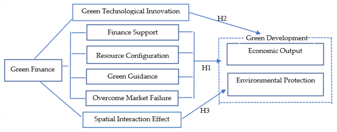
2. Theoretical Analysis and Research Hypotheses

The essence of the relationship between green finance and green development is the relationship between finance, the economy, and the environment. Green development emphasizes the unification and coordination of economic development and environmental protection. Green finance refers to economic activities concerning environmental improvement and resource conservation, which promotes the development of financial products such as green credit, green bonds, and green stocks through policy mechanisms to gain environmental, economic, and social benefits. It is important to accelerate the green development of the economy to support the construction of ecological civilization. Specifically, green finance has an effect on green development, mainly through the following three ways:

First, green finance has a direct effect on green development by providing financial support, improving resource allocation, instigating the green guidance action, and overcoming market failures. First of all, green finance has a financial support function. The financial system has functions such as improving risks, promoting information acquisition and resource allocation, strengthening corporate control, and mobilizing savings according to the study of Levine [33]. On one hand, green finance provides financial supports for the operation of green projects, environmental pollution control, and ecological construction and restoration. On the other hand, green finance provides financial support for the production and sales of the green environmental protection industry on a larger scale, which can increase economic output by taking environmental protection into account. Second of all, green finance has also a resource allocation function. Bai et al. [34] pointed out that resource allocation is the core function of finance. Green finance combines the resource allocation function of the financial industry with environmental and social responsibilities, and guides society to shift the focus of investment to high-tech, energy-saving environmental protection by transferring funds from high energy-consuming, heavy-polluting industries, and to environmentally friendly green industries. For enterprises of heavy pollution with strong innovation capabilities, they will accelerate the development and application of green production technology and production equipment to achieve green transformation and upgrading. Furthermore, heavy-polluting and low-efficiency companies will fail to survive without funds, leading them to “shut down”. No matter which type, the pollution emissions in the market will gradually be weakened, and the green industry will gradually be cultivated and strengthened. Therefore, it is possible to increase green output while reducing pollution. In addition, the development of green finance has a strong incentive and plays a guiding role in enhancing the endogenous nature of the green development for enterprises. In recent years, China has vigorously supported the development of green finance by supporting policies and related laws and regulations in the financial field, fiscal field, and environmental protection field, etc., which have released signals of green development for enterprises to guide enterprises to actively adjust production and operation decisions in accordance with national policy to enhance their own green development capabilities. Finally, green finance can effectively overcome market failures. Environmental pollution has strong externalities, which can easily lead to market failures. Relying on the government’s post-penalty intervention to make up for market failures may bring problems such as local protectionism and inefficiency. Green finance can combine environmental risks with financial risks by making full use of financial risk management techniques. With the help of market mechanisms and social supervision, green finance can effectively overcome market failures to change post-event punishment into pre-event prevention or mid-event supervision. It should be noted that, for those regions mainly relying on the heavy chemical industries, pollution has been suppressed to a certain extent due to green finance restricting funds flowing to heavy chemical industries, along with the reduction in local economic output. Therefore, green finance may have a negative effect on local green development in this case.

The second effect green finance has on green development is its support of green technological innovation. From a micro perspective, green development is inseparable from the support of green enterprises such as new technology, new energy, new materials, energy saving, and environmental protection. Green finance is likely to guide resources to tilt towards such enterprises, enabling them to obtain financing at a lower cost. Green finance also supports R&D for such enterprises in product design, production, and other links, towards breakthroughs in green industry fields such as energy conservation, environmental protection, clean production, and clean energy. In addition, by supporting large-scale green technological innovation, with the reduction in costs and prices of green production, green consumption, and green travel, green economic activities have more cost and price advantages than non-green economic activities, which has resulted in the promotion of the allocation of resources to green industries really using market mechanisms and price mechanisms. Therefore, green finance can promote the green transformation of investment, production, and consumption without relying on government subsidies. It should be noted that, in regions with low levels of green technological innovation, large-scale green technological innovation has not been formed, and the development of green production (such as clean energy or electric vehicles) and green consumption (such as energy-saving appliances or green buildings) are limited, leading to excessively high costs for green products and services. Coupled with the characteristics of the long cycle and high risk of green technological innovation, the realization of commercial profits requires a long time and comes with a high cost. Therefore, green finance cannot promote green development by supporting green technological innovation in regions with low levels of green technology innovation.

Thirdly, green finance has spatial spillover effects on green development. According to the growth pole theory put forward by Perroux [32], in the initial development stage of green finance, regions with a high level of green finance development will attract financial resources from surrounding regions, which leads to a lack of funds to support the development of green enterprises in surrounding regions, but improves the local level of green finance, which is manifested as a polarization effect. This turns out to be a positive spatial spillover effect of green finance on green development under these circumstances. When the development of green finance reaches a certain stage, regions with higher levels of green finance will export financial resources to surrounding regions, which will radiate and drive the development of green finance in surrounding regions, so that surrounding regions have sufficient funds to support the development of local green enterprises, which is manifested as a diffusion effect. It turns out to be negative spatial spillover effect of green finance on green development under these circumstances.

Based on the above analysis, we propose the following hypotheses:

Hypothesis 1 (H1):

Green finance can promote regional green development, but for regions mainly relying on the development of high-energy-consuming and high-polluting industries, green finance may have a negative effect on local green development.

Hypothesis 2 (H2):

Green finance can have a positive effect on regional green development by supporting green technological innovation, but in regions with a low level of green technological innovation, the effect may be negative.

Hypothesis 3 (H3):

The impact of green finance on green development has spatial spillover effects. Whether the spatial spillover effects are positive or negative depends on the level of local green finance development.

In summary, the theoretical and mechanistic analyses of the hypotheses are shown in Figure 1.

3. Study Design

3.1. Measurement of Green Development

Green development emphasizes not only economic output but also environmental protection, with the core feature to achieve higher economic output with the least resource input and environmental pollution as possible. In the existing literature related to green development, similar concepts involved are eco-efficiency [35,36,37,38], environmental efficiency [39,40], and green economic efficiency [41,42]. On this basis, taking into account the core characteristics of green development of the existing literature, the regional eco-efficiency will be selected as the measure of regional green development. As a nonparametric method, the form of the frontier production function is not needed by data envelopment analysis (DEA) [43], which can effectively deal with multiple inputs and outputs. In addition, the effectiveness has nothing to do with the units of the variables. Therefore, we use the super-efficiency slacks-based measure (SBM) model [44], which is an extended model based on the DEA method combined with the window analysis to measure the comparable eco-efficiency of the 30 provincial administrative regions from 2007 to 2019 in both cross-section and time series, which has been used in Ye et al. [38]. A more detailed understanding of the principle and advantages of this method will be given in Section 3.1.1 and Section 3.1.2.

3.1.1. Super-Efficiency SBM Model

The SBM model has been proposed by Tone [45] as an expansion model of DEA, which uses a non-ray method to introduce the slack variable into the objective function directly. With all the slack variables taken into account, the efficiency value can be evaluated more accurately. However, the SBM model is the same as the traditional DEA model, which cannot discriminate between plural decision-making units (DMUs) with the full “efficient status”. Later, Tone further proposed the super-efficiency SBM model [44], which appears to discriminate between these efficient DMUs. The super-efficiency SBM integrates the advantages of the super-efficient DEA model and the SBM model. Which is supposed to make further discriminations between the efficient DMUs at the frontier under the conditions of undesirable outputs. Based on study of Tone [44], we regard each region as a DMU with a total of n DMUs, and each DMU is equipped with m input (including the capital input, physical resource input and human resource input), a desired output $s_1$, and an undesirable output $s_2$, which are represented, respectively, by the matrices as $X=\left(x_{ij}\right)\in R^{m\times n}$, $Y^g=\left(y_{ij}^g\right)\in R^{s_1\times n}$, and $Y^b=\left(y_{ij}^b\right)\in R^{s_1\times n}$, where $x_{ij}$ is the variable for i-th input variables of the j-th DMU, $y_{ij}^g$ as the variable for i-th desired output variables of the j-th DMU, and $y_{ij}^b$ as the variable for i-th undesirable output variables of the j-th DMU. The super-efficiency issue has been discussed under the assumption that the DMU $\left(x_0,y_0\right)$ is SBM-efficient. Let a production possibility set $P\backslash \left(x_0,y_0\right)$ as

$$P\backslash \left(x_0,y_0\right)=\left\{\left(\overline{x},\overline{y}\right)|\overline{x}\ge {\displaystyle \sum _{j=1,\ne 0}^n{\lambda }_j{x}_j},\overline{y}\le {\displaystyle \sum _{j=1,\ne 0}^n{\lambda }_j{y}_j},\overline{y}\ge 0,\lambda \ge 0\right\}$$

Further, a subset $\overline{P}\backslash \left(x_0,y_0\right)$ of $P\backslash \left(x_0,y_0\right)$ is defined as

$$\overline{P}\backslash \left(x_0,y_0\right)=P\backslash \left(x_0,y_0\right)\cap \left\{\overline{x}\ge x_0 \mathrm{and} \overline{y}\le y_0\right\}$$

The super-efficiency of $\left(x_0,y_0\right)$ is defined as the optimal objective function value ${\delta }^{\ast }$ of the following Model (1):

$$\begin{array}{l}{\delta }^{\ast }=\min \frac{\frac{1}{m}{\displaystyle \sum _{i=1}^m\frac{{\overline{x}}_i}{x_{i0}}}}{\frac{1}{s_1+s_2}\left({\displaystyle \sum _{r=1}^{s_1}\frac{{\overline{y}}_r^g}{y_{r0}^g}+{\displaystyle \sum _{r=1}^{s_2}\frac{{\overline{y}}_r^b}{y_{r0}^b}}}\right)}\\ \mathrm{s}.\mathrm{t}. \left\{\begin{array}{c}\overline{x}\ge {\displaystyle \sum _{j=1,\ne 0}^n{\lambda }_j{x}_j}\\ {\overline{y}}^g\le {\displaystyle \sum _{j=1,\ne 0}^n{\lambda }_j{y}_j^g}\\ {\overline{y}}^b\ge {\displaystyle \sum _{j=1,\ne 0}^n{\lambda }_j{y}_j^b}\\ \overline{x}\ge x_0,{\overline{y}}^g\le y_0^g,{\overline{y}}^b\le y_0^b,\lambda \ge 0\end{array}\right.\end{array}$$

(1)

where $\lambda$ refers to the weight vector and $\left(x_0,y_0^g,y_0^b\right)$ are denoted as the input, desired output, and undesirable output of a certain DMU, respectively.

$$\begin{array}{l}{\tau }^{\ast }=\min \tau =\frac{1}{m}{\displaystyle \sum _{i=1}^m\frac{{\overline{x}}_i}{x_{i0}}}\\ \mathrm{s}.\mathrm{t}. \left\{\begin{array}{c}1=\frac{1}{s_1+s_2}\left({\displaystyle \sum _{r=1}^{s_1}\frac{{\tilde{y}}_r^g}{y_{r0}^g}+{\displaystyle \sum _{r=1}^{s_2}\frac{{\tilde{y}}_r^b}{y_{r0}^b}}}\right)\\ \tilde{x}\ge {\displaystyle \sum _{j=1,\ne 0}^n{\mathsf{\Lambda }}_j{x}_j}\\ {\tilde{y}}^g\le {\displaystyle \sum _{j=1,\ne 0}^n{\mathsf{\Lambda }}_j{y}_j^g}\\ {\tilde{y}}^b\ge {\displaystyle \sum _{j=1,\ne 0}^n{\mathsf{\Lambda }}_j{y}_j^b}\\ \tilde{x}\ge t{x}_0 \mathrm{and} \tilde{y}\ge t{y}_0\\ \mathsf{\Lambda }\ge 0,\tilde{y}\ge 0,t>0\end{array}\right.\end{array}$$

(2)

According to the analysis by Tone [44], let $\left(\alpha x_0,\beta y_0\right)$ with $\alpha \le 1$ and $\beta \ge 1$ be a DMU with reducing inputs, followed by enlarging the desirable outputs and reducing the undesirable outputs as $\left(x_0,y_0\right)$. Then, the super-efficiency score of $\left(\alpha x_0,\beta y_0\right)$ is not less than that of $\left(x_0,y_0\right)$.The fractional program, like super-efficiency SBM, can be transformed into a linear programming problem by the Charnes–Cooper transformation as in [43,46]:

According to the analysis by Tone [44], let an optimal solution of Model (2) be $\left({\tau }^{\ast },{\tilde{x}}^{\ast },{\tilde{y}}^{\ast },{\mathsf{\Lambda }}^{\ast },t^{\ast }\right)$. An optimal solution of the super-efficiency SBM can be expressed as

$${\delta }^{\ast }={\tau }^{\ast },{\lambda }^{\ast }={\mathsf{\Lambda }}^{\ast }/t^{\ast },{\overline{x}}^{\ast }={\tilde{x}}^{\ast }/t^{\ast },{\overline{y}}^{\ast }={\tilde{y}}^{\ast }/t^{\ast }$$

3.1.2. Super-Efficiency SBM Window Model

According to Model (2), it is useful to solve the problem of input and output slacks and discriminate efficient DMUs. However, Model (2) is a static model, which does not perform cross-sectional efficiency of the DMUs over time; this can be addressed effectively by the DEA window analysis method.

The DEA window analysis method, proposed by Charnes et al. [47], is useful for efficient measurements by treating DMUs of a different period as different DMUs on the principle of the moving average. In the DEA window analysis framework, it compares the eco-efficiency of a DMU in a certain period not only with that of the other DMUs in the same period, but also with its own eco-efficiency in other periods. The key feature to notice is the selection of the window width is sized to either $d=3$ or $d=4$, it demonstrates a better balance in terms of reliability and stability of the efficiency measure. If there are DMUs of size n with the window width of $d$, it is certain to have a DMU of size $d\times n$ in one window. On the assumption of the total time length of $T$, windows of size $T-d+1$ for each DMU are required to measure the efficiency, with an efficiency value of size d in any window.

The moving average method shows that, for each DMU window, the efficiency values of size d on each window are measured accordingly starting from the first time point $t=1$ to the second time point $t=2$ untill $T-d+1$, but the final result of the evaluated DMU is predicted by the average efficiency value at each time point. The specific operation method is shown in

Table 1. The window analysis of a DMU in period $T(d=3)$.

Windows	$\mathit{t}-1$	$\mathit{t}-2$	$\mathit{t}-3$	$\mathit{t}-4$	$\mathit{t}=5$	…	$\mathit{t}=\mathit{T}-4$	$\mathit{t}=\mathit{T}-3$	$\mathit{t}=\mathit{T}-2$	$\mathit{t}=\mathit{T}-1$	$\mathit{t}=\mathit{T}$
1	${\mathrm{E}}_{11}$	${\mathrm{E}}_{12}$	${\mathrm{E}}_{13}$
2		${\mathrm{E}}_{21}$	${\mathrm{E}}_{22}$	${\mathrm{E}}_{23}$
3			${\mathrm{E}}_{31}$	${\mathrm{E}}_{32}$	${\mathrm{E}}_{33}$
…						…
$T-d-1$							${\mathrm{E}}_{T-d-1,1}$	${\mathrm{E}}_{T-d-1,2}$	${\mathrm{E}}_{T-d-1,3}$
$T-d$								${\mathrm{E}}_{T-d,1}$	${\mathrm{E}}_{T-d,2}$	${\mathrm{E}}_{T-d,3}$
$T-d+1$									${\mathrm{E}}_{T-d+1,1}$	${\mathrm{E}}_{T-d+1,2}$	${\mathrm{E}}_{T-d+1,3}$
Average value

.

Then, similar to the study of Ye et al. [38], we construct a super-efficiency SBM window model (i.e., slacks-based measure of super-efficiency model combining with the window analysis). The eco-efficiency ${\mathrm{E}}_{st}$ of a DMU at the time $\begin{array}{cc}t& (t=1,2,\cdots ,d)\end{array}$ within the window $\begin{array}{cc}s& (s=1,2,\cdots ,T-d+1)\end{array}$ expressed by a super-efficiency SBM model is shown as follows:

$$\begin{gathered} {\mathrm{E}}_{st}=\min \frac{\frac{1}{m}{\displaystyle \sum _{i=1}^m\frac{{\overline{x}}_i^{st}}{x_{i0}^{st}}}}{\frac{1}{s_1+s_2}\left({\displaystyle \sum _{r=1}^{s_1}\frac{{\overline{y}}_r^{g,st}}{y_{r0}^{g,st}}+{\displaystyle \sum _{r=1}^{s_2}\frac{{\overline{y}}_r^{b,st}}{y_{r0}^{b,st}}}}\right)} \\ \mathrm{s}.\mathrm{t}.\left\{\begin{array}{c}{\overline{x}}^{st}\ge {\displaystyle \sum _{j=1,0}^{d\times n}}{\lambda }_j^{sr}{x}_j^{st} \\ {\overline{y}}^{g,st}\ge {\displaystyle \sum _{j=1,0}^{d\times n}}{\lambda }_j^{sr}{y}_j^{g,st} \\ {\overline{y}}^{b,st}\ge {\displaystyle \sum _{j=1,0}^{d\times n}}{\lambda }_j^{sr}{y}_j^{b,st} \\ {\overline{x}}^{st}\ge x_0^{st},{\overline{y}}^{g,st}\le y_0^{g,st},{\overline{y}}^{b,st}\le y_0^{b,st},{\lambda }_j^{st}\ge 0\end{array}\right. \end{gathered}$$

(3)

where $j=1,2,\cdots ,d\times n;s=1,2,\cdots ,T-d+1,t=1,2,\cdots ,d$, the meanings of all the variables are basically in accordance with Model (1). More precisely, the superscript (subscript) st demonstrates the variable at the time point of $t$ within the window of s. As an example of $x_j^{st}$, it indicates the input vector of the DMU $j$ at the time of $t$ within the window of $s$. In this paper, Model (3) suggests the evaluation of the comparable eco-efficiency of China’s 30 provincial administrative regions from 2007 to 2019 in both the cross-sectional and time series. Regarding the availability of relevant data, an index system is constructed to evaluate the eco-efficiency in three dimensions of input, desired output, and undesirable output, shown in

Table 2. Eco-efficiency evaluation index system.

Tier 1 Indicators	Secondary Indicators	Tertiary Indicators (Unit)
Input	Capital investment	Investment in Fixed Assets (CNY 10,000)
	Resource input	Energy Consumption (10,000 tce)
		Water Supply (10,000 tons)
		Area of Land Used for Urban Construction (square kilometer) Cultivated Area (square kilometer)
		Employment (10,000 people)
Desirable output	Regional development indicators	Regional Gross Domestic Product (CNY 10,000)
Undesirable output	Environmental benefit indicators	Volume of Industrial Wastewater Discharged (10,000 tons)
		Volume of Sulphur Dioxide Emission (ton)
		Volume of Industrial Dust Emission (ton)

.

The indicators of eco-efficiency reflecting resource constraints mainly is composed of the capital input and resource input. Among them, the capital input is converted into stock data based on 2007 by using the perpetual inventory calculation method. The resource input is mainly performed with involvement of energy, water resources, land resources and human resources, which prefers the option of energy consumption to the total amount of standard coal converted by electricity, gas and liquefied petroleum gas. The area of land used for urban construction and cultivated area is chosen to measure the input of land resources. In addition, the consumption of water resources is presented by the total amount of water consumption, while the human resource input is measured by employment.

The eco-efficiency output indicator is composed of desired output indicators and undesirable output indicators. The former is the regional development indicator measured by the gross regional product (GDP is converted to constant prices based on 2007 in the actual calculation), the latter for environmental benefits. With a view toward the availability of the data, the environmental constraints are represented by industrial wastewater discharged, sulfur dioxide emission and industrial dust emission.

3.2. Measurement of Green Finance

Regarding the measurement of the development level of green finance, we should transform complex practical phenomena into simple and effective information. At present, there is no unified method in academia. Five secondary indicators of green finance have evaluated in the book “China Green Finance Report 2014” written by Li et al. [48] say: green credit, green securities, green insurance, green investment, and carbon finance, which is more comprehensively to put the financial products and financial instruments into green finance. Therefore, the method prevails among subsequent studies because it can more scientifically reflect the development level of green finance. Based on the study of Li et al. [48], considering the availability of data and the definition of green finance comprehensively, this paper constructs a comprehensive evaluation system for green finance at the provincial level from the perspective of the overall development of green finance. The specific indicators and descriptions are shown in

Table 3. Evaluation Index System for the Development Level of Green Finance.

First Level Indicators	Secondary Indicators	Definition
Green credit	Proportion of interest expenditure of high-energy-consumption industries	Interest expenditures of the six high- energy- consuming industries/total interest expenditures of industrial industries
Green securities	Market value of environmental protection enterprises	Market value of environmental protection enterprises /total market value of A shares
	Market value of high-energy- consuming industries	Market value of the six high-energy-consuming industries/total market value of A shares
Green insurance	Proportion of agricultural insurance scale	Agricultural insurance expenditure/total insurance expenditure
	Compensation rate of agricultural insurance	Agricultural insurance expenditure/agricultural insurance income
Green investment	Proportion of energy-saving and environmental protection expenditure	Energy-saving and environmental protection industry fiscal expenditure/total fiscal expenditure
	Percentage of investment in environmental pollution control	Investment in pollution control /GDP

.

The first indicator is green credit. As the proportion of green credit published by commercial banks is national level, green credit is measured by the inverse indicator of the percentage of the interest expenditures of the six high-energy-consumption industries in the total industrial industry interest expenditures in this paper. All relevant data come from the China Industrial Statistical Yearbook and Statistical Yearbooks of various regions. Second, green securities are measured by the percentage of market value of energy-saving and environmentally friendly enterprises and the percentage of market value of the six high-energy-consuming industries. For the selection of energy-saving and environmentally friendly enterprises, this paper refers to the classification of energy-saving and environmentally friendly industries on the Tonghuashun website as the standard. The six high-energy-consuming industries is composed of the non-ferrous metal smelting and rolling processing industry, the petroleum processing coking and nuclear fuel processing industry, the chemical raw material and chemical product manufacturing industry, the ferrous metal smelting and rolling processing industry, the non-metallic mineral products industry, and the electricity and heat production and supply industry. The data of the market value of energy-saving and environmentally friendly enterprises, the market value of the six high-energy-consuming industries, and the total market value of A-shares all come from the CSMAR database. The next indicator is green insurance. China formally established the institutional framework of environmental pollution liability insurance in 2007. At present, the development of green insurance is still in the preliminary stage, and the relevant data are not complete. Therefore, this paper replaces the scale of environmental liability insurance and the compensation rate of environmental liability insurance with those of agricultural insurance as a measure of green insurance. The source of these data is from the China Insurance Yearbook. Last is green investment, which can be measured by two indicators: the proportion of the energy-saving and environmental protection fiscal expenditure within the total fiscal expenditure and the proportion of pollution control investment in GDP. Among them, the data of energy conservation and environmental protection fiscal expenditure, total fiscal expenditure, and GDP can be found from the Statistical Yearbook of each province, and the pollution control investment from the China Environmental Statistical Yearbook. Finally, we use the entropy method to synthesize the green finance index as a measure of the development level of green finance. The larger the green finance index is, the higher the development level of green finance will be. As China officially established the institutional framework for environmental pollution liability insurance in 2007, we choose 2007 as the starting year for green finance evaluation, with the ending year of 2019, for which data are currently available.

3.3. Variables, Methodology and Data

3.3.1. Explanatory Variables

Green finance (gf) is the core explanatory variable. The entropy method is used to synthesize the green finance index as the measurement of green finance. The evaluation index system for the development level of green finance used is shown in Table 3. In addition, in order to explore whether green finance can promote green development by supporting green technological innovation, we have taken the interactive product term of green finance and green technological innovation as core explanatory variables. The specific method to analyze promotion of green finance on green development by supporting green technological will be given in Section 3.3.2.

As for the control variables, we consider the following. First, green technological innovation (gti) has an effect on eco-efficiency by reducing environmental pollution in the production process, through green innovation technologies at the front end of the production process and governance technologies at the back end of the production process. Regarding the measurement of the level of green technological innovation, in line with the measurements provided by Costantini et al. [49], we manually searched the green patent applications and green patent authorizations of various provinces (autonomous regions or municipalities) from the website of the State Intellectual Property Office of China (SIPO) according to the “Green Patent IPC Classification Number” in the International Patent Green Classification List launched by the World Intellectual Property Organization (WIPO) in 2010. We add 1 to this variable and take the natural logarithm in the empirical models in order to eliminate the influence of heteroscedasticity. Secondly, as seen in the studies by He and Zhang [50] and Yu et al. [51], there is a significant correlation between the level of economic development and environmental quality, so a natural logarithm (lnpgdp) of real GDP per capita has been included in the model to control the impact of economic development levels on eco-efficiency. Third, the pollution level is closely related to the energy structure according to the empirical research conclusions of Ma and Zhang [52], so an energy consumption structure (es) has been included in the model. The energy consumption structure is measured by the proportion of coal consumption in total energy consumption. Fourth, according to the analysis of Jorgenson [53], with the help of FDI, less developed countries appear to be “pollution refuges” to environmental degradation while developing rapidly. Then, the proportion of foreign investment in the model is needed to define the regional openness (open) to control the impact of openness on the eco-efficiency. Finally, according to the research of Ge et al. [54], urbanization has a significant impact on pollution emissions, and we added the urbanization rate (urb) to the model to capture the effect of urbanization on the eco-efficiency.

3.3.2. Spatial Panel Data Model

According to the growth pole theory [32] mentioned in Section 1 and Section 2, the impact of green finance on regional eco-efficiency may have spatial spillover effects, so a spatial econometric model is necessary to analyze the impact of various variables on eco-efficiency. Based on the research of Elhorst [55], we use the spatial Durbin model (abbreviated as SDM), with the endogenous spatial interaction effect and the spatial interaction effect of the disturbance term. The SDM of the impact of green finance on eco-efficiency is constructed as follows:

$$\begin{array}{l}{\mathrm{EE}}_{it}={\alpha }_i+\rho {\displaystyle \sum _{j=1}^{30}{w}_{ij}}{\mathrm{EE}}_{jt}+{\beta }_1\times {\mathrm{gf}}_{it}+{\beta }_2\times {\mathrm{gf}}_{it}\times \ln \left({\mathrm{gti}}_{it}+1\right)+{\beta }_3{X}_{it}+{\displaystyle \sum _{j=1}^{30}{w}_{ij}}{\mathrm{gf}}_{jt}\times {\theta }_1\\ \begin{array}{cc}& \end{array}+{\displaystyle \sum _{j=1}^{30}{w}_{ij}}{\mathrm{gf}}_{it}\times \ln \left({\mathrm{gti}}_{it}+1\right)\times {\theta }_2+{\displaystyle \sum _{j=1}^{30}{w}_{ij}}{X}_{it}\times {\theta }_3+u_i+v_t+{\epsilon }_{it}\end{array}$$

(4)

First, the LM test is used to determine whether there is a significant spatial effect. If not, the traditional panel OLS regression is applicable. The model is as follows:

$${\mathrm{EE}}_{it}={\alpha }_i+{\beta }_1\times {\mathrm{gf}}_{it}+{\beta }_2\times {\mathrm{gf}}_{it}\times \ln \left({\mathrm{gti}}_{it}+1\right)+{\beta }_3{X}_{it}+u_i+v_t+{\epsilon }_{it}$$

(5)

If the LM test judges that there is a significant spatial effect, the LR test is used to determine whether the SDM can be degenerated into a spatial lag model (abbreviated as SAR) (as the following Model (6)) or degenerated into a spatial error model (abbreviated as SEM) (as the following Model (7)):

$${\mathrm{EE}}_{it}={\alpha }_i+\rho {\displaystyle \sum _{j=1}^{30}{w}_{ij}}{\mathrm{EE}}_{jt}+{\beta }_1\times {\mathrm{gf}}_{it}+{\beta }_2\times {\mathrm{gf}}_{it}\times \ln \left({\mathrm{gti}}_{it}+1\right)+{\beta }_3{X}_{it}+u_i+v_t+{\epsilon }_{it}$$

(6)

$$\begin{array}{l}{\mathrm{EE}}_{it}={\alpha }_i+{\beta }_1\times {\mathrm{gf}}_{it}+{\beta }_2\times {\mathrm{gf}}_{it}\times \ln \left({\mathrm{gti}}_{it}+1\right)+{\beta }_3{X}_{it}+u_i+v_t+{\epsilon }_{it}\\ {\epsilon }_{it}=\lambda {\displaystyle \sum _{j=1}^{30}{w}_{ij}}{\epsilon }_{jt}+{\mu }_{it}\end{array}$$

(7)

Note that in the above Models (4)–(7), EE is the eco-efficiency, which represents the level of green development. gf means the green finance index to show green finance development. $X$ indicates the control variable vector as described in Section 3.3.1. $\mathrm{gf}\times \ln \left(\mathrm{gti}+1\right)$ indicates the interactive item of green finance and green technological innovation, which is used to judge the indirect effect of green finance on green development by supporting green technological innovation. If the sign is significantly positive, it means that green finance can promote green development by supporting green technological innovation; if not, it means that the impact of green finance on green development by supporting green technological innovation is not significant; if it is significantly negative, it means that the support of green finance for green technological innovation has a negative effect on green development. $\mathrm{W}={\left({\mathrm{w}}_{\mathrm{ij}}\right)}_{30\times 30}$ is constructed as the spatial weight matrix, based on the queen adjacency relationship; specifically: if city i is adjacent to city j in geographic space, let ${\mathrm{W}}_{\mathrm{ij}}=1$. Otherwise, let ${\mathrm{W}}_{\mathrm{ij}}=0$. In addition, ${\mathrm{W}}_{\mathrm{ii}}=0$. $\delta$ is the spatial autoregressive coefficient, $\lambda$ the spatial autocorrelation coefficient, $\beta$ the regression coefficient for explanatory variable, and $\theta$ the regression coefficient for space lagged term of explanatory variable. $u_i$ is known as the individual effect and can be set in a fixed or random form. If it is a fixed effect, then ${\displaystyle \sum _{i=1}^{30}{u}_i}=0$. If it is a random effect, $u$ and $\epsilon$ are not related. $v_t$ is the time effect, ${\epsilon }_{it}$ the random error term, and ${\alpha }_i$ as the constant term, while i and j represent city and year, respectively.

3.3.3. Samples and Data Sources

The main data sources of this paper are list as follows: The data for measuring eco-efficiency are all from Statistical Yearbooks of various provinces (autonomous regions or municipalities) except for the energy data from the China Energy Statistical Yearbook over the years. Green patent data are searched from the website of the State Intellectual Property Office (SIPO). The data for green credit are from the China Industrial Statistical Yearbook and the Statistical Yearbooks of various provinces (autonomous regions and municipalities), green securities from the CSMAR database, and green insurance from the China Insurance Yearbook over the years. As for the data for measuring green investment, the pollution control investment data are from the China Environmental Statistical Yearbook over the years, and the others from the Statistical Yearbooks of various provinces (autonomous regions and municipalities) over the years. In addition, China officially established the institutional framework for environmental pollution liability insurance in 2007. For the consistency of the sample data period, we set the period of research starting from 2007 to 2019. A small amount of missing data are filled in by interpolation method, and all variables related to price are adjusted to a constant price based on 2007.

The research sample for this paper is 30 provincial administrative regions in Mainland China. Due to China’s vast territory, there are significant differences in the economic development, green finance development, and green technological innovation levels of the eastern, central, and western regions, and the effect of green finance on eco-efficiency will also vary. Therefore, according to the balance of the sample size and the similarity of the economic and financial levels, this paper will also conduct a subregional study based on the traditional method of dividing China into three economic zones. The eastern region includes 11 provincial-level administrative regions: Beijing, Tianjin, Hebei, Liaoning, Shanghai, Jiangsu, Zhejiang, Fujian, Shandong, Guangdong, and Hainan; the central region consists 8 provincial-level administrative regions: Shanxi, Jilin, Heilongjiang, Anhui, Jiangxi, Henan, Hubei, and Hunan Administrative region; and the west region contains 11 provincial administrative regions: Inner Mongolia, Guangxi, Sichuan, Chongqing, Guizhou, Yunnan, Shaanxi, Gansu, Qinghai, Ningxia, and Xinjiang (due to limitation of data availability, Tibet, Hong Kong, Macao, and Taiwan have been excluded).

4. Empirical Results of the Models and Discussion

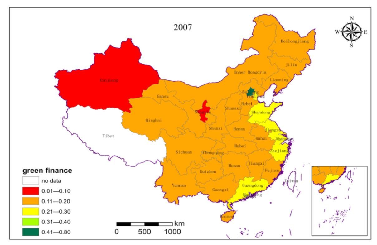
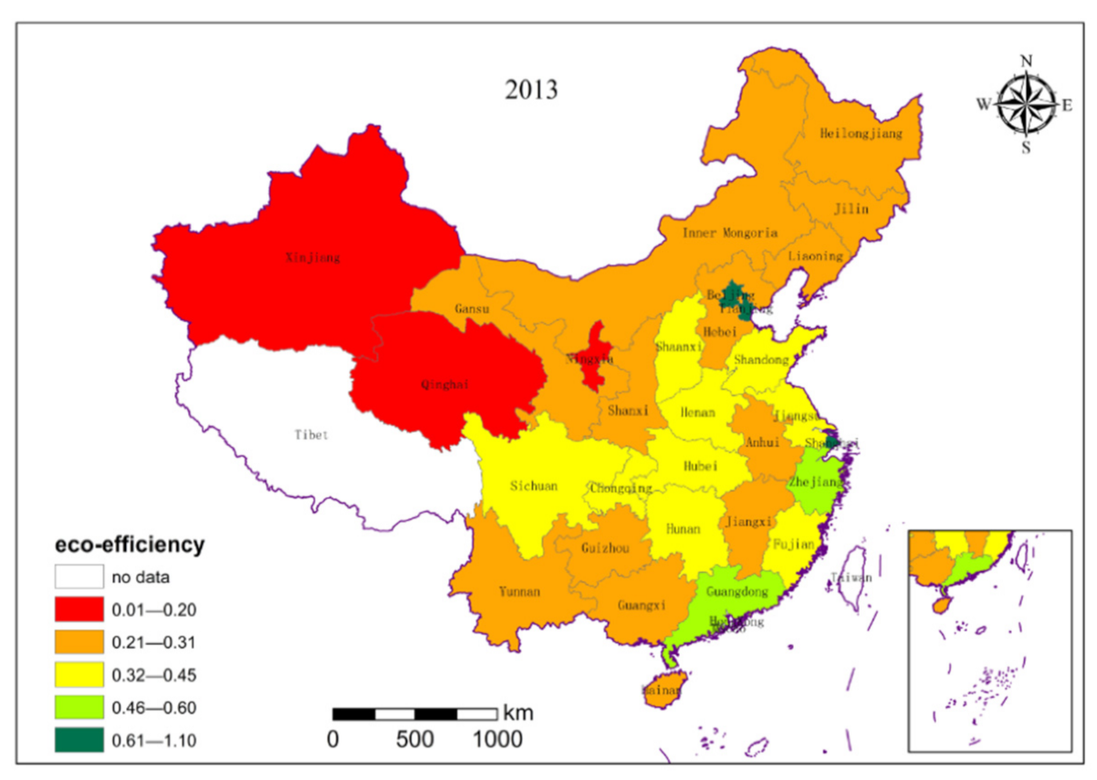
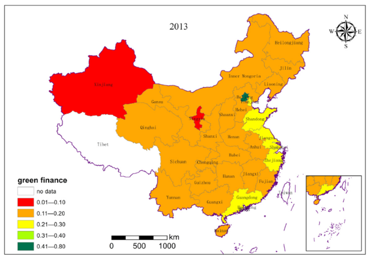
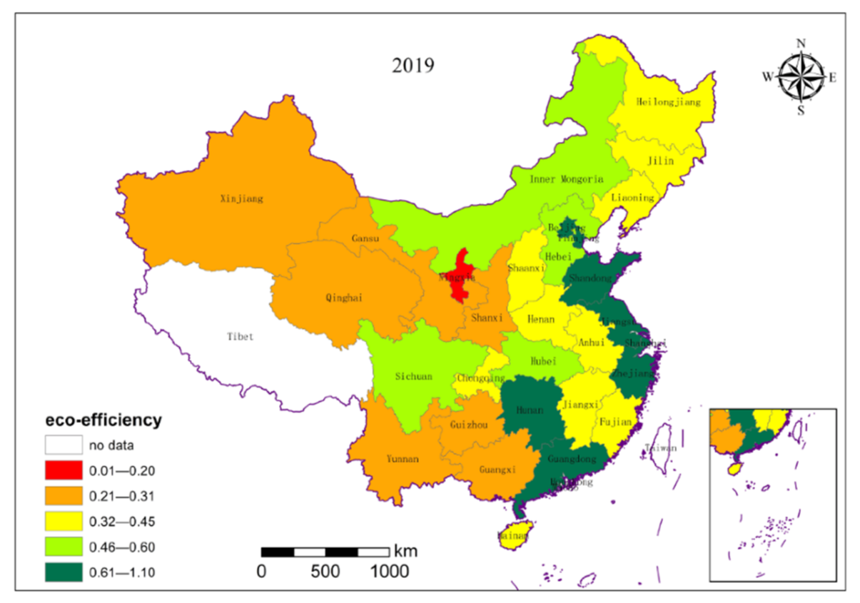
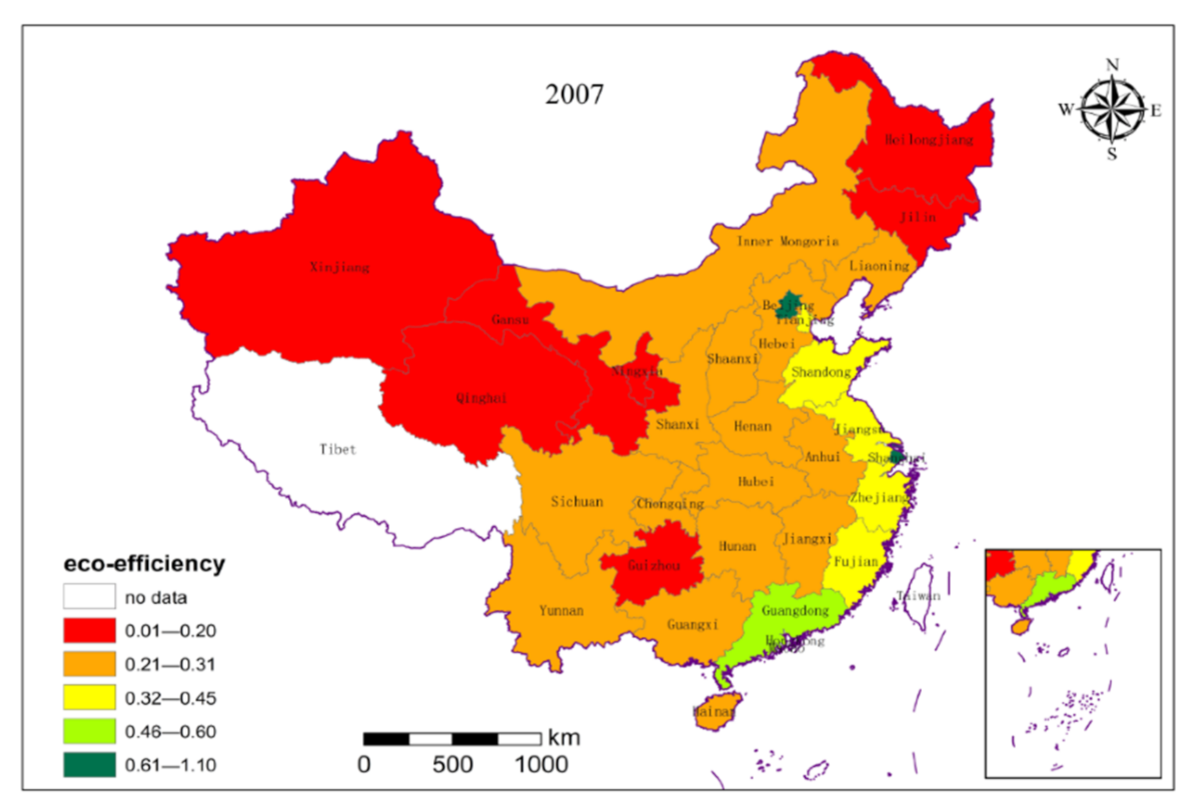
4.1. The Temporal and Spatial Changes and Connection of Regional Green Finance and Eco-Efficiency

We naturally grade eco-efficiency and green finance index of China’s provinces in 2007, 2013 and 2019 using ArcGIS software, as shown in Figure 2, Figure 3, Figure 4, Figure 5, Figure 6 and Figure 7.

Comparing these figures, we can intuitively see the temporal and spatial changes and connections between China’s provincial eco-efficiency and the development of green finance. It can be seen that, in recent years, the awareness of “green development” is committed to the way of development armed with green sensibility, as is the eco-efficiency of all provinces across the country with significant difference. From the figures in the given three years, the eco-efficiency of Beijing and the eastern coastal regions are relatively high, while the western and northeastern regions are always at low-value clusters. Hunan and Hubei provinces from the central region, and Sichuan province from the western region have improved significantly in recent years. Similarly, the regions with high green finance are distributed in Beijing or the eastern coastal regions. Most of the western, central, and northeastern regions are at low-value clusters. Hunan, Hubei from the central region, and Sichuan, Chongqing, and Shaanxi from the western region show a significant jump. Comparing the distribution of eco-efficiency and green finance, it can be seen that regions with higher levels of eco-efficiency are at higher green finance level, such as Beijing, Shanghai, Jiangsu, Zhejiang, and Guangdong. Provinces with low eco-efficiency are at low green finance level, such as Xinjiang, Qinghai, and Ningxia from the western region, and Shanxi, Jilin, and Heilongjiang from the central region. These similarities in the distribution of eco-efficiency and green finance have indicated the spatial correlation between these two indexes.

Observing Figure 2, Figure 3, Figure 4, Figure 5, Figure 6 and Figure 7, we can also find that regions with neighbors of higher green finance tend to have lower green finance. For example, the green finance of Beijing has always been at the forefront of the country during these years, but the green finance of Hebei, adjacent to Beijing, is at a relatively low level. As another example, the green finance of Guangdong is always at a high level these years, but the green finance of Guangxi, which adjacent to Guangdong, is at a relatively low level, which implies that green financial resources are formed in areas with better financial and economic development. Thus, green finance resources have formed agglomerations in regions with well-developed finance and economics, which find it easy to attract resources from underdeveloped regions, that is, the polarization effect. A similar agglomeration phenomenon happens to eco-efficiency. However, this is not always the case. For example, the development level of green finance is very high in Beijing, as well as in Tianjin, adjacent to Beijing. Similarly, the development level of green finance is high in Shanghai and also in Jiangsu and Zhejiang, both adjacent to Shanghai. A similar situation also occurs in the neighboring provinces of Guangdong and Hunan. This phenomenon implies the existence of the diffusion effect. Based on the above intuitive analysis using graphics, we can conclude that green finance may have spatial interaction effects on green development.

The results of spatial correlation between the dependent variable and core independent variable have been reported in

Table 4. The spatial correlation of eco-efficiency and green finance in 2019.

Variables	Moran’I	p-Value	Geary’s c	p-Value
EE	0.227	0.009	0.570	0.003
GF	0.146	0.023	0.460	0.029

, that is, eco-efficiency and green finance, respectively, in 2019. Both the Moran’I and Geary’s c indicators show that eco-efficiency and green finance have a significant spatial correlation at the 5% level, which further illustrates the necessity of spatial econometric models to analyze the relationship between green finance and eco-efficiency.

4.2. Results and Discussion

4.2.1. Selection of Model and Estimation Methods

Firstly, the LM test is used to determine whether to apply the ordinary least squares regression or the spatial econometric model. According to the results in

Table 5. Regression results of the SDM model (point estimation).

Variable	Whole Country	East Region	Central Region	West Region
W × EE	0.1486 ** (2.03)	0.1531 * (1.82)	−0.3776 ***(−3.50)	−0.3863 ***(−3.18)
gf	0.3015 * (1.80)	0.2240 ** (2.22)	1.8536 (1.36)	−0.6275 * (−1.88)
gf × ln (gti + 1)	0.0722 ** (2.30)	0.1622 ** (2.57)	−0.0881 (−0.41)	−0.1291 * (1.82)
ln (gti + 1)	−0.0072 (−0.86)	0.0629 *** (3.20)	−0.0096 (−0.33)	−0.0201 * (−1.68)
open	0.0015 (0.15)	0.0086 (0.66)	0.3463 *** (5.29)	−0.0037 (−0.09)
urb	0.3553 *** (3.46)	0.3922 ** (2.18)	−0.2478 (−1.20)	−0.9677 ***(−3.30)
es	−0.0435 ***(−2.71)	0.3238 *** (2.99)	0.1196 ** (2.10)	−0.0248 (−1.56)
lnpgdp	0.1803 *** (6.83)	0.2176 *** (3.22)	0.3490 *** (5.38)	0.3053 *** (8.66)
W × gf	−2.8247 ***(−5.39)	2.1068 (1.11)	1.9274 (1.09)	−0.8361 * (−1.77)
W × gf × ln (gti + 1)	−0.2078 ***(−2.62)	0.2168 (1.49)	−0.4642 * (−1.66)	−0.2174 * (1.72)
W × lngti	0.0223 (1.09)	0.0714 ** (2.05)	0.0731 * (1.70)	−0.0163 (−0.86)
W × open	0.0910 *** (4.16)	−0.0590 * (−1.90)	−0.0432 (−0.32)	0.1019 (1.55)
W × urb	−0.0452 (−0.27)	0.6740 ** (2.36)	0.1537 (0.26)	−1.8368 ***(−4.19)
W × es	−0.0028 (−0.09)	0.7092 *** (3.85)	−0.0918 (−1.44)	−0.0589 ** (−2.08)
W × lnpgdp	0.1816 *** (3.44)	−0.1921 (−1.62)	0.5633 *** (4.38)	0.1753 ** (2.46)
R2	0.6827	0.8467	0.2041	0.5095
LogL	459.4799	177.2615	237.3615	331.9666
${\sigma }^2$	0.0055 ***	0.0049 ***	0.0005 ***	0.0005 ***
LM-test	29.391 ***	7.444 ***	8.625 ***	11.111 ***
LR_spatial_lag	31.12 ***	27.05 ***	53.31 ***	41.53 ***
LR_spatial_err	37.88 ***	27.10 ***	34.82 ***	16.32 ***
Hausman-test	37.50 ***	35.33 ***	36.11 ***	34.29 ***

Note: The t-statistic are in parentheses. ***, **, and * indicate significance at the 1%, 5%, and 10% levels, respectively.

, the statistics of the LM test are significant at the 1% level, indicating the significant spatial correlation to apply spatial measurement model. To determine the form of the spatial panel model, an LR test is used to determine whether the SDM can be degenerated into SAR or SEM. The LR statistics of the model in Table 5 are significant at the 1% level, indicating that SDM is a more suitable model. In addition, the Hausman test is significant at the 1% level, indicating that a fixed-effects model is needed. Based on the above series of tests, we finally choose the SDM model with time fixed and individual fixed as the benchmark model. The regression results of the model are shown in Table 5.

Most previous research on spatial effects have applied the point estimation of spatial models to examine spatial spillover effects. LeSage and Pace [56] pointed out that point estimation is prone to errors. It is recommended to obtain the average spillover effect from the perspective of solving partial differential equations. Additionally, Elhorst [57] suggested that this method provides a more effective way and lays solid foundation for measuring and testing spatial spillover effects. Therefore, we will use this method to study the spatial spillover effects of green finance. In addition, LeSage and Pace [56] defined the influence of the independent variable on the dependent variable in local as a direct effect and in neighboring regions as an indirect effect; this is the spatial spillover effect. Moreover, according to LeSage and Pace [56], the mean value method is used to measure the direct effect, the indirect effect, and the total effect. Elhorst and Fréret [58] further put forward the statistical test method of the effect.

The analysis of the decomposition results of direct effects, indirect effects, and total effects is effective to study spatial effects, a method which is widely used in later literatures. In the following analysis, we will also use direct effects, indirect effects, and total effects to analyze the spatial effects of green finance and other variables on eco-efficiency. The results of the direct effects, indirect effects, and total effects, measured based on the SDM model when the dependent variable is eco-efficiency, have been reported in

Table 6. Spatial effect decomposition based on the adjacent space weight matrix.

	Variable	Nationwide	Eastern Region	Central Region	Western Region
Direct Effect	gf	0.2044 (1.13)	0.3908 ** (2.12)	1.6379 (1.13)	−0.5457 * (−1.78)
	gf × ln (gti + 1)	0.0793 (1.02)	0.1461 ** (2.12)	0.0009 (0.00)	−0.2111 ** (−2.32)
	ln (gti + 1)	−0.0065 (−0.78)	0.0584 *** (2.85)	−0.0275 (−0.89)	−0.0195 ** (−2.21)
	Open	0.0058 (0.62)	0.0060 (0.46)	0.3926 *** (5.45)	−0.0095 *** (−3.22)
	Urb	0.3491 *** (3.49)	0.4401 ** (2.49)	−0.3109 (−1.21)	−0.8347 *** (−2.69)
	es	−0.0433 *** (−2.73)	−0.3872 *** (−3.36)	0.1515 *** (2.75)	−0.0202 (−1.34)
	lnpgdp	0.1896 *** (7.35)	0.2113 *** (2.95)	0.2590 *** (4.12)	0.3018 *** (7.92)
Indirect Effect	gf	−3.2098 *** (−5.02)	0.1789 *** (3.07)	1.1209 (0.72)	−0.3184 ** (−2.35)
	gf × ln (gti + 1)	−0.2537 *** (−2.88)	0.1120 ** (2.25)	−0.3979 (−1.66)	−0.1391 * (−1.79)
	ln (gti + 1)	0.0243 (1.07)	0.0696 * (1.81)	0.0747 (1.01)	−0.0065 (−0.37)
	open	0.1052 (1.14)	−0.0626 * (−1.77)	−0.1608 (−1.26)	0.0832 (1.44)
	urb	0.0105 (0.05)	0.3063 ** (2.56)	0.2389 (0.43)	−0.2026 (−1.07)
	es	−0.0104 (−0.26)	−0.8632 (−1.04)	−0.1248 ** (−2.04)	−0.0386 * (−1.66)
	lnpgdp	0.2381 (1.17)	0.1666 ** (2.17)	0.1070 *** (3.39)	0.0462 (0.85)
Total Effect	gf	−3.0054 ** (−2.28)	0.5697 ** (2.48)	2.7588 (1.53)	−0.8641 * (−1.75)
	gf × ln (gti + 1)	−0.1744 ** (−2.13)	0.2581 ** (2.29)	−0.3971 (−1.37)	−0.3502 * (−1.72)
	ln (gti + 1)	0.0178 (0.70)	0.0112 (0.22)	0.0473 (1.20)	−0.0260 ** (−2.50)
	open	0.1110 (0.98)	−0.0566 (−1.39)	0.2317 ** (2.06)	0.0737 (1.54)
	urb	0.3596 ** (2.21)	0.7464 ** (2.22)	−0.0720 (−0.15)	−1.0373 ** (−2.23)
	es	−0.0536 * (−1.92)	−1.2504 * (−1.88)	0.0266 (0.35)	−0.0588 ** (−2.21)
	lnpgdp	0.4277 ** (2.36)	0.3779 ** (2.22)	0.3660 *** (5.17)	0.3480 *** (7.52)

Note: The t-statistic are in parentheses. ***, **, and * indicate significance at the 1%, 5%, and 10% levels, respectively.

.

4.2.2. Nationwide

From a national perspective, in terms of direct effects, the coefficient for gf is positive, but not significant. The reason for this may be that, from a national perspective, gf can provide financial support for the operation of green projects and the development of environmental protection and new energy industries, and guide funds from industries with high energy consumption and heavy pollution to environmentally friendly ones. However, for regions with high-energy-consumption and heavily-polluting industries as the main source of economic output, the reduction in the financial support for their main industries will undoubtedly lead to a reduction in economic output. Although certain environmental benefits have been achieved, the economic benefits have been greatly reduced. Therefore, the comprehensive effect of gf on EE is not significant, which has confirmed the second half of H1 in Section 2. In addition, the coefficient for gf × ln (gti + 1) is positive, but not significant, that is, the effect of gf on EE by supporting gti is not significant. The reason for this may be that, from a national perspective, the level of gti is still relatively low, and green production technology and pollution control technology are not yet mature; along with the characteristics of long cycle and high risks, it is definite that green finance cannot improve EE by supporting gti, which has confirmed the second half of H2 in Section 2.

In terms of indirect effects, the coefficient for gf is −3.2098 and significant at the 1% level (t = −5.02), which means that a 1% increase in gf causes a 3.2098% decrease for EE in the neighborhood when other variables remain unchanged. The coefficient for gf × ln (gti + 1) is −0.2537 and significant at the 1% level (t = −2.88), which means that a 1% increase in gf × ln (gti + 1) causes a 0.2537% decrease for EE in the neighborhood when other variables remain unchanged, which is proven to result in a polarization effect. Taking Beijing in 2019 as an example, the green finance index is 0.793 according to the measurement in Section 3.2. However, the green finance index of Hebei, adjacent to Beijing, is only 0.161. Similarly, the green finance index of Guangdong is 0.402, while Jiangxi, adjacent to Guangdong, is only 0.162. According to the growth pole theory [32], regions with a higher level of green finance will absorb the surrounding financial resources, resulting in a lack of funds to support the operation of green projects the development of green industries in neighboring regions, and the R&D and innovation of green enterprises. Therefore, from a national perspective, the spatial spillover effect of gf is significantly negative, as is gf by supporting gti, which supports H3 in Section 2.

For control variables, the direct effect and the indirect effect of gti are both not significant, which means that the gti fails to show a positive role in promoting EE nationally. The reason may be that the level of gti is relatively low and green products are absent of price advantages. The direct effect and the indirect effect of open are both not significant. The reason for this may be that the introduction of foreign capital and technology has caused a reduction in environmental effect due to the “pollution paradise” effect at the time during the period of economic growth from a national perspective. The direct effect of urb is significantly positive at the 1% level. It shows that from a nationwide perspective, a large number of human resources have flowed to cities, which is very beneficial to the improvement of EE. However, the indirect effect of urb is not significant. The direct effect of es is significantly negative at the 1% level, indicating that the energy consumption structure dominated by coal has increased pollution emissions nationally, which is not conducive to promote EE in the local region. However, the spatial spillover effect of es is not significant. The direct effect of lnpgdp is positive and significant at the 1% level, indicating that lnpgdp can effectively promote EE in the local region. The spatial spillover effect of lnpgdp is not significant.

4.2.3. Eastern Region

From the perspective of the eastern region, in terms of direct effects, the coefficient for gf is 0.3908 and significant at the 5% level (t = 2.12), which means that a 1% increase in gf causes a 0.3908% increase for EE in the local region when other variables remain unchanged. Possible reasons for this are as follows. The provinces are relatively well-developed in the eastern region. Taking Beijing, Shanghai, Jiangsu, Zhejiang, and Guangdong as examples, the main sources for economic growth have transitioned from high-energy-consuming and heavily-polluting industries to high-tech, energy-saving, and environmentally-friendly industries in these regions. Green finance has provided an effective financial way to support the development of high-tech, energy-saving, and environmentally-friendly industries in these regions. In addition, due to the function of resource allocation of green finance, financial institutions provide credit support to green industries and green projects. At the same time, the development of the high-energy-consuming and heavily-polluting industries are curbed. As a result, the increasing green output reduces pollution, thereby EE is improved, which verifies the first half of H1 in Section 2. The coefficient for gf × ln (gti + 1) is 0.1461 and significant at the 5% level (t = 2.12), which means that a 1% increase in gf × ln (gti + 1) causes a 0.1461% increase for EE in the local region when other variables remain unchanged. This suggests that in eastern China, gti has reached a certain level. The cost and price of green economic activities such as green production and green consumption have shown advantages compared with non-green economic activities. Therefore, it is natural for gf to increase the output of green economy but reduce environmental pollution by supporting gti. That is, gf can promote eco-efficiency by supporting gti, which verifies the second part of H2 in Section 2.

In terms of indirect effects, the coefficient for gf is 0.1789 and significant at the 1% level (t = 3.07), which means that a 1% increase in gf causes a 0.1789% increase for EE in the neighborhood when other variables remain unchanged. The coefficient for gf × ln (gti + 1) is 0.1120 and significant at the 5% level (t = 2.25), which means that a 1% increase in gf × ln (gti + 1) causes a 0.1120% increase for EE in the neighborhood when other variables remain unchanged. The reason for this may be related to the diffusion effect. For most provinces in eastern China, the green finance has reached a certain level. Taking Beijing, Shanghai, Jiangsu, Zhejiang, and Guangdong in 2019 as examples, the green finance indexes are 0.793, 0.377, 0.336, 0.339, and 0.402, respectively, according to the measurement in Section 3.2. Obviously, the development of gf has reached a certain level in these regions, so financial resources will be exported to surrounding regions to drive the development of gf in surrounding regions. In this way, sufficient funds are available to support green environmental protection industries as well as innovation funds for green enterprises to promote eco-efficiency in the neighborhood. Therefore, gf and gf × ln (gti + 1) show significantly positive spatial spillover effects in the eastern region, which has verified H3 in Section 2.

For control variables, the direct effect and the indirect effect of gti are both significantly positive. The reason for this may be that the level of gti has reached a certain level, which has begun to promote green development. The direct effect of open is positive but not significant. The possible reasons are as follows: the introduction of foreign capital and technology has aggravated environmental pollution for the “pollution paradise” effect during the period of economic growth. The indirect effect of open is significantly negative at the 10% level. The direct effect and the indirect effect of urb on EE are both significantly positive at the 5% level. The direct effect of es is significantly negative at the 1% level, indicating that the energy consumption structure dominated by coal has led to an increase in pollution emissions. The indirect effect of es is not significant. The direct effect and indirect effect of lnpgdp are positive, and significant at the 1% level and 5% level, respectively, indicating that high level of lnpgdp can effectively promote EE not only in the local regions, but also in the neighborhood.

4.2.4. Central Region

From the perspective of the central region, in terms of direct effects, the effect of gf on EE is positive but not significant. The reason for this may be that: the development of gf limits funds flowing to pollution-intensive industries transferred from the eastern coastal provinces such as the non-ferrous metal mining and dressing industry, non-metallic mining and dressing industry, textile industry, paper industry, petroleum processing industry, and coking and nuclear fuel processing industry which have become the leading industries in the central region of China after implementing the strategy for the rise of central China in 2004. This is bound to reduce the economic output of the central region. In addition, gf can provide certain financial supports for green industry with no obvious economic or environmental benefits because green industry is still in the initial stage of development in the central region. Therefore, the effect of gf on EE is not significant, which has confirmed the second half of H1 in Section 2. The effect of gf on EE by supporting gti is very weak and not significant. This may be due to the fact that the gti in central China has not yet reached a certain level, coupled with the characteristics of long cycle and high risks, leading to the insignificant effect of gf on EE by supporting gti, which has confirmed the second half of H2 in Section 2.

In terms of indirect effects, the coefficients for gf and gf × ln (gti + 1) are both not significant, which indicates the insignificant spatial spillover effects of gf on EE, as well as the effect of gf on EE by supporting gti. The possible reasons for this are as follows: the green finance indexes among provinces in the central regions are not much different. Taking 2019 as an example, the green finance indexes of top three provinces are 0.202 (Hunan), 0.198 (Hubei), and 0.186 (Henan), while the green finance indexes of the lowest three provinces are 0.142 (Heilongjiang), 0.145 (Shanxi), and 0.147 (Jilin) according to the measurement in Section 3.2. As the level of green finance of the provinces in the central region is not high without difference, the spatial spillover effect of gf is not significant according to the growth pole theory [32], as is the effect of gf by supporting gti, which illustrates H3 in Section 2.

For control variables, the direct effect and the indirect effect of gti are both not significant. This may be due to the fact that the level of gti is insufficient, which does not yet show its role in promoting EE. The direct effect of open is significantly positive at the 1% level, showing that the introduction of foreign resources and technology is effective to promote EE in the local region. The indirect effect of open is not significant. The direct effect and the indirect effect of urb are both not significant. The reason for this may be that the influx of a large number of laborers into cities is conducive to the development of economic output, along with the increasing of pollution emissions. Therefore, the comprehensive effect of urb on EE is not significant. The direct effect of es is significantly positive at the 1% level, indicating that the higher the proportion of coal in energy consumption is, the more economic output in central China there will be. The spatial spillover effect of es is not significant. The direct effect and indirect effect of lnpgdp is significantly positive at the 1% level, indicating that lnpgdp can effectively promote EE both in the local region and neighborhood.

4.2.5. Western Region

From the perspective of the western region, in terms of direct effects, the coefficient for gf is −0.5457 and significant at the 10% level (t = −1.78), which means that a 1% increase in gf causes a 0.5457% decrease for EE in the local region when other variables remain unchanged. This is as the economic development strategy of the western region has always prioritized the development way of resource extraction and processing and the raw material industry for a long time. Economic growth in the western region mainly depends on extractive industry and raw material industry, such as coal mining and washing, oil and natural gas mining, ferrous and non-ferrous metal mining and processing, non-metallic mineral products, ferrous and non-ferrous metal smelting and rolling processing and petroleum processing. The development of green finance will inevitably reduce the financial support for these industries, definitely leading to a reduction in economic output in the western region. In addition, the development of green industry is still very weak in the western region with little economic and environmental benefits. Therefore, green finance has a negative effect on eco-efficiency, which confirms the second half of H1 in Section 2. The coefficient for gf × ln (gti + 1) is −0.2111 and significant at the 5% level (t = −2.32), which means that a 1% increase in gf × ln (gti + 1) causes a 0.2111% decrease for EE in the local region when other variables remain unchanged. The possible reasons for this are as follows: the level of green technological innovation in the western region is still relatively low, with the limited effect of green production technology and pollution control technology on the improvement of the ecological environment. In addition, green technological innovation has the characteristics of a long cycle and high risk, which has weakened the price advantage of green production and green consumption. In this case, the financial support for green technological innovation cannot bring out its economic benefits, so the overall impact on eco-efficiency is negative, which has confirmed the second half of H2 in Section 2.

In terms of indirect effects, the coefficient for gf is −0.3184 and significant at the 5% level (t = −2.35), which means that a 1% increase in gf causes a 0.3184% decrease for EE in the neighborhood when other variables remain unchanged. The coefficient for gf × ln (gti + 1) is −0.1391 and significant at the 10% level (t = −1.79), which means that a 1% increase in gf × ln (gti + 1) causes a 0.1391% decrease for EE in the neighborhood when other variables remain unchanged. The spatial spillover effect of gf is significantly negative at the 5% level, and the spatial spillover effect of gf by supporting gti is significantly negative at the 10% level. This phenomenon may be related to the polarization effect. The level of green finance is relatively low in the western region. In 2019, Shaanxi, Sichuan, and Chongqing ranked the top three for green finance with 0.218, 0.215, and 0.211, respectively, while Xinjiang, Ningxia, and Yunnan ranked as the bottom three, with only 0.097, 0.103, and 0.140, respectively, according to the measurement of green finance in Section 3.2. On the basis of the financial growth pole theory proposed by Perroux [32], in the initial stage of finance, regions with a higher level of green finance will absorb in surrounding financial resources, leading to a lack of sufficient funds to support the operation of green projects, the development of green industries, and the R&D of green enterprises in surrounding areas, which manifests as a polarization effect. Therefore, the spatial spillover effect of gf is significantly negative, as is gf × ln (gti + 1), which verifies H3 in Section 2.

For control variables, the direct effect of gti is significantly negative at the 5% level. The reason may be that green technological innovation is still at the initial stage in the western region, with the limited economic benefits and environmental benefits brought by green technological innovation. On the contrary, economic output will be reduced due to the immaturity of the green technology market. The indirect effect of gti is not significant. The direct effect of open is significantly negative at the 1% level. The possible reasons are as follows: the introduction of foreign resources and technology has increased local economic output to a certain extent, along with the increasing of pollution emissions due to the transfer of international high-polluting industries. Comparing these two, the comprehensive effect of open on eco-efficiency is negative. The indirect effect of open is not significant. The direct effect of urb is significantly negative at the 1% level, while the indirect effect is not significant. The direct effect of es is negative, but not significant. The spatial spillover effect of es is significantly negative at the 10% level, due to the pollution diffusion effect. The direct effect of lnpgdp is significantly positive at the 1% level, indicating that lnpgdp can effectively promote EE in the local region. However, the spatial spillover effect of lnpgdp is not significant.

5. Control for Endogeneity and Robustness Test

5.1. Control for Endogeneity

As for endogeneity, based on the differences from the variables in the time and spatial dimension, the period effect and spatial fixed effect models have been applied to control for unobservable factor errors caused by the time factor and unit factor (see Lesage [56]; Lin and Liu [59]; and Chong [60]). In particular, in Chapter 2 of the study proposed by Lesage’s book [56], Lesage points out that the omitted variables motivation is one of the motives for the introduction of spatial econometric model. In Chapter 3 of the research proposed by Lesage’s book [56], Lesage further expounds that the ML estimation of spatial model can alleviate the biased problem of estimation, which can reduce the endogenous problem. We then verify the endogenous problems caused by interaction to ascertain the presence of reverse causality. According to the method in Liu et al. [61], the dependent variable (EE) and core explanatory variables (gf) are exchanged to evaluate the endogeneity caused by reverse causality nationwide and in the eastern region, central region, and western region. The empirical outcomes (see

Table 7. Endogenous test caused by reverse causality (the effect of EE on gf).

	Variable	Nationwide	Eastern Region	Central Region	Western Region
Direct Effect	EE	−0.0431 (0.87)	0.0403 (0.26)	0.0156 (0.97)	−0.0228 (−1.48)
	gf × ln (gti + 1)	0.1301 *** (5.52)	0.1202 *** (8.43)	0.1491 *** (9.13)	0.0976 *** (9.31)
	ln (gti + 1)	−0.0304 (1.43)	−0.0329 (−1.52)	−0.0169 (−0.34)	−0.0129 (−0.22)
	open	0.0009 (0.75)	−0.0026 (−1.61)	−0.0108 ** (−2.16)	−0.0011 (−0.19)
	urb	0.1197 *** (4.49)	0.1206 ** (2.11)	0.0267 (1.59)	−0.0698 (−1.60)
	es	−0.0104 ** (−2.53)	−0.1215 *** (−4.85)	−0.0001 (−0.03)	−0.0043 * (−1.84)
	lnpgdp	0.0029 ** (2.42)	0.0042 *** (3.21)	0.0031 (0.52)	0.0059 (0.94)
Indirect Effect	EE	−0.0698 (−1.06)	0.0278 (1.01)	0.0450 (0.26)	−0.0735 (−0.92)
	gf × ln (gti + 1)	0.0070 (1.21)	−0.0151 ** (−2.28)	0.0271 (3.68)	−0.0776 *** (−5.67)
	ln (gti + 1)	0.0005 (0.20)	0.0092 (0.97)	−0.0017 (−0.94)	0.0108 (3.52)
	open	−0.0010 (−0.39)	0.0030 (0.79)	−0.0096 (−1.03)	0.0046 (0.30)
	urb	0.2512 ** (2.29)	0.4507 ** (2.10)	0.0462 (1.13)	0.0832 (0.95)
	es	0.0139 * (1.83)	0.0645 * (1.86)	0.0023 (0.48)	−0.0010 (−0.20)
	lnpgdp	0.0053 (0.60)	0.0013 (0.09)	−0.0451 (−0.53)	0.0211 (1.48)
Total Effect	EE	−0.1129 (−0.93)	0.0125 (0.67)	0.0606 (0.90)	−0.0963 (−0.42)
	gf × ln (gti + 1)	0.1371 *** (4.46)	0.1051 *** (4.02)	0.1761 (7.61)	0.0200 (1.25)
	ln (gti + 1)	−0.0299 (1.04)	−0.0329 (−1.01)	−0.0186 * (−1.82)	−0.0021 (−0.64)
	open	−0.0000 (−0.01)	0.0004 (0.11)	−0.0204 ** (−2.00)	0.0035 (0.21)
	urb	0.3708 *** (4.95)	0.5712 ** (2.23)	0.0729 (1.64)	0.0134 (0.13)
	es	0.0035 (0.42)	−0.0571 (−1.43)	0.0022 (0.28)	−0.0053 (−0.82)
	lnpgdp	0.0082 ** (2.13)	0.0055 ** (2.17)	−0.0420 (−0.12)	0.0271 (1.57)

Note: The t-statistic are in parentheses. ***, **, and * indicate significance at the 1%, 5%, and 10% levels, respectively.

) show that the effects of EE on gf are not significant. Thus, we contend that, as a whole, the endogenous problems caused by reverse causality are not significant.

5.2. Robustness Test

In order to ensure the reliability of the above analysis results, we have performed the following two robustness tests in this section: one is to change the measurement method of the dependent variable and the other is to change the construction method of the spatial weight matrix. The results and analysis of the two robustness tests will be reported in the following two subsections.

5.2.1. Change the Measurement of the Dependent Variable

As the economical utilization of energy can reflect “more output and less pollution” to a certain extent, we use the ratio of total energy consumption (data from the China Energy Statistical Yearbook) to represent the GDP of each province (autonomous regions and municipalities), that is, energy consumption per unit of GDP, as a measure of green development for robustness testing. After a series of tests such as the LM test, LR test, and Hausman test, the dual-fixed SDM model is still proven to be the best tool to explore the impact of green finance on energy consumption per unit of GDP in the whole country, eastern region, central region, and western region. The results of spatial effect decomposition are reported in

Table 8. The spatial effect decomposition of changing the measurement method of the dependent variable.

	Variable	Nationwide	Eastern Region	Central Region	Western Region
Direct Effect	gf	1.1168 (1.40)	0.3888 ** (2.63)	6.4147 (0.47)	−11.6059 *** (−9.02)
	gf × ln (gti + 1)	0.1635 (1.57)	0.1688 ** (2.20)	−1.6805 *** (−4.64)	−2.8523 *** (−5.95)
	ln (gti + 1)	0.0725 (1.43)	0.0309 ** (2.21)	−0.2194 *** (4.01)	−0.4783 *** (−4.28)
	open	−0.0924 *** (−4.34)	−0.0767 *** (−5.53)	−0.4253 *** (−2.99)	−0.3018 (−0.63)
	urb	0.4751 (1.04)	0.1113 (0.29)	1.6042 *** (3.53)	9.7687 *** (6.92)
	es	−1.0090 *** (−13.78)	−0.1987 (−0.81)	−0.6372 *** (−5.76)	−0.5000 *** (−4.22)
	lnpgdp	1.0236 *** (8.90)	0.6025 *** (4.97)	0.7042 *** (6.30)	1.8106 *** (6.52)
Indirect Effect	gf	−0.8546 ** (−2.41)	0.1224 * (1.69)	3.4151 (1.04)	−5.2027 *** (−2.75)
	gf × ln (gti + 1)	−0.0909 * (−1.92)	0.0540 ** (2.11)	−0.6042 (−1.39)	−1.5727 *** (−3.11)
	ln (gti + 1)	−0.0130 (−0.33)	0.0098 * (1.91)	−0.0794 (−1.28)	0.2590 (1.39)
	open	0.0197 (0.41)	0.0252 *** (3.35)	0.5640 ** (2.26)	1.1550 (1.46)
	urb	3.3415 *** (4.91)	−0.0356 (−0.28)	0.5441 (0.44)	−8.5091 *** (−4.24)
	es	0.3383 ** (2.27)	0.0654 (0.79)	0.0618 (0.48)	−0.6394 *** (−2.99)
	lnpgdp	−0.3128 ** (−2.31)	0.1977 *** (3.28)	−0.2599 (−1.26)	−1.5486 *** (−3.60)
Total Effect	gf	0.2622 (1.25)	0.5112 * (1.93)	9.8298 (1.43)	−16.8086 *** (−3.41)
	gf × ln (gti + 1)	−0.0726 (−1.46)	0.2228 ** (2.10)	−2.2847 ** (−2.50)	−4.4250 *** (0.30)
	ln (gti + 1)	0.0594 (1.52)	0.0407 * (1.90)	−0.2988 *** (−2.77)	−0.2193 (−1.40)
	open	−0.0727 (−1.46)	−0.0515 *** (−5.38)	0.1387 (0.56)	0.8533 (1.03)
	urb	3.8165 *** (4.61)	0.0758 (0.29)	2.1483 * (1.68)	1.2596 (0.50)
	es	−0.6707 *** (−3.98)	−0.1333 (−0.81)	−0.5754 *** (−3.18)	−1.1394 *** (−4.89)
	lnpgdp	0.7108 *** (9.06)	0.8002 *** (4.84)	0.4443 *** (4.38)	0.2620 ** (2.29)

Note: The t-statistic are in parentheses. ***, **, and * indicate significance at the 1%, 5%, and 10% levels, respectively.

.

Comparing Table 8 with Table 6, we can see that the direct and indirect effects of the core explanatory variables of gf and gf × ln (gti + 1) maintain a high degree of consistency except the following nuances: for the central sample, the coefficient of direct effect on gf × ln (gti + 1) is significantly negative at the 1% level in Table 8, while it is close to 0 and not significant in Table 6. In addition, comparing the coefficients for all control variables in Table 6 and Table 8, the sign or significance of a few variables have been changed, but the change can be ignored, which does not affect our research conclusions. According to the above analysis, even if the measurement method of green development is changed, the effect of green finance on the eco-efficiency has basically not been changed for national sample, eastern sample, central sample, and western sample; this also hold true to the effect of green finance by supporting green technological innovation, which has shown the robustness of the conclusions.

5.2.2. Change the Way the Spatial Weight Is Constructed

Considering that the regression results of the spatial econometric model are very sensitive to the construction method of the spatial weight matrix, we have changed the method of constructing the spatial weight matrix based on the queen adjacency relationship. In this subsection, we construct the spatial weight matrix based on the inverse distance function for robustness testing, in which the distance between the two provincial administrative regions can be calculated based on the latitude and longitude coordinates of the government resident, followed by the reciprocal. The results of spatial effect decomposition based on inverse distance function space weight matrix are reported in

Table 9. The spatial effect decomposition based on inverse distance function space weight matrix.

	Variable	Nationwide	Eastern Region	Central Region	Western Region
Direct Effect	gf	0.4570 (11.15)	1.2304 *** (2.68)	0.1311 (0.10)	−1.4923 *** (−2.62)
	gf × ln (gti + 1)	0.0708 (0.95)	0.1367 * (1.90)	0.1503 (0.75)	−0.2102 *** (−3.30)
	ln (gti + 1)	−0.0146 (−1.59)	0.0629 *** (3.09)	−0.0484 * (−1.68)	−0.0331 *** (−2.88)
	open	0.0117 (1.14)	−0.0579 *** (−3.52)	0.3249 *** (4.69)	−0.0306 (−0.68)
	urb	0.0475 (0.47)	1.5297 *** (6.10)	−0.2534 (−1.07)	−1.6272 *** (−5.01)
	es	−0.0681 *** (−3.88)	−0.7571 *** (−5.20)	0.0764 (1.50)	0.0807 ** (2.27)
	lnpgdp	0.2462 *** (8.72)	0.1645 * (1.66)	0.2977 *** (3.40)	0.2568 *** (6.25)
Indirect Effect	gf	−1.8850 (−1.43)	0.9980 ** (2.38)	−1.1281 (−0.76)	−0.0548 ** (−2.36)
	gf × ln (gti + 1)	−0.1646 ** (2.16)	0.1523 ** (2.18)	0.1315 (0.59)	−0.0347 ** (−2.33)
	ln (gti + 1)	0.0485 (0.86)	0.0570 (0.83)	0.0170 (0.55)	0.0146 (0.90)
	open	0.1907 *** (2.93)	−0.4122 *** (−4.36)	−0.0918 (−0.89)	0.1203 (1.01)
	urb	−0.1842 (−0.29)	0.6980 *** (4.90)	−2.2384 *** (−4.65)	0.7249 (1.18)
	es	−0.0683 (−0.59)	2.8809 (0.76)	−0.1848 *** (−2.64)	−0.0432 ** (−2.24)
	lnpgdp	0.2097 (0.90)	0.0726 *** (3.53)	0.1040 ** (2.57)	−0.0094 (−0.13)
Total Effect	gf	−1.4280 (−1.02)	2.2284 *** (2.63)	−0.9970 (−1.09)	−1.5471 *** (−2.93)
	gf × ln (gti + 1)	−0.0938 (1.05)	0.2890 ** (2.15)	0.2818 (1.06)	−0.2449 *** (2.82)
	ln (gti + 1)	0.0339 (0.57)	0.1199 (0.07)	−0.0313 ** (−2.45)	−0.0184 (−1.50)
	open	0.2025 *** (3.04)	−0.4701 *** (−4.40)	0.2331 *** (3.23)	0.0897 (1.19)
	urb	−0.1367 (−0.21)	2.2277 *** (4.10)	−2.4918 *** (−5.73)	−0.9023 ** (−2.02)
	es	−0.1363 (−1.14)	2.1238 (1.19)	−0.1084 (−1.63)	0.0375 * (1.89)
	lnpgdp	0.4559 * (1.89)	0.2371 ** (2.27)	0.4017 *** (6.73)	0.2474 *** (3.57)

Note: The t-statistic are in parentheses. ***, **, and * indicate significance at the 1%, 5%, and 10% levels, respectively.

.

Comparing Table 9 with Table 6, we can see that the direct and indirect effects of the core explanatory variables of gf and gf × ln (gti + 1) maintain a high degree of consistency except for the following nuances: for the national sample, the result of indirect effect of gf is different in Table 6 and Table 8. The coefficient for gf is not significant in Table 9, while it is significantly negative at the 1% level in Table 6. For the central sample, the signs of the indirect effects of gf and gf × ln (gti + 1) are both inconsistent, and not significant in Table 6 and Table 9, so there is no significant difference. In addition, comparing the coefficients for all control variables in Table 6 and Table 9, the sign or significance of a few variables have been changed, but this does not affect our research conclusions and can therefore be ignored. According to the above analysis, even if the method of constructing the spatial weight matrix is changed, the effects of green finance on the eco-efficiency has basically not been changed for the national, eastern, central, and western samples; this is also true for the effect of green finance by supporting green technological innovation, which has shown the robustness of the conclusions.

6. Conclusions and Further Research

6.1. Conclusions

As the core of the economy, finance is an important aspect of green development in China. As the People’s Bank of China and other seven ministries and commissions have jointly issued the “Guiding Opinions” in 2016, green finance has a tendency of rapid development in China. Firstly, after summarizing relevant references on the impact of green finance on the economy and society from the micro level to the macro level, the main issues proposed in this paper are the effects of green finance on green development and the effects of green finance on green development by supporting green technological innovation. Secondly, this paper has analyzed the theoretical mechanism of green finance influencing green development and green finance influencing green development by supporting green technological innovation. Thirdly, the super-efficiency SBM window analysis model has been applied to make a scientific and reasonable measurement of the green development of 30 provincial administrative regions in Mainland China from 2007 to 2019, and a green finance evaluation index system has been constructed using the entropy method to synthesize a green finance index as measurement of the green finance of each provincial administrative region from 2007 to 2019. Fourthly, this paper has selected the SDM model to produce empirical research to analyze the direct and indirect effects of green finance on green development and green finance on green development by supporting green technological innovation through spatial effect decomposition. Finally, robustness tests have been conducted by changing the measurement method of green development and the setting of the spatial weight matrix to prove the robustness of the conclusions. The main conclusions obtained in this paper are summarized as follows:

First, the levels of green development and green finance in China from 2007 to 2019 have shown an overall upward trend, with obvious regional differences. The green development of Beijing and the eastern coastal provinces are at a leading level, while it has always been a low-value cluster in the western and northeastern regions. The level of green development has been greatly improved in central regions such as Hunan and Hubei and western regions such as Sichuan in recent years. The level of green finance is similar to the level of green development. The regions with a higher green finance index are concentrated in Beijing and the eastern coastal provinces such as Shanghai, Jiangsu, Zhejiang, and Guangdong, as opposed to the lower regions located in the western region, such as Xinjiang, Qinghai and Ningxia, and the central region, such as Shanxi, Jilin and Heilongjiang, which has proven the spatial interaction between green development and green finance.

Secondly, the spatial effects of green finance on green development are different in the eastern, central, and western regions and nationwide. In terms of direct effects, green finance has shown a significant positive effect on green development in the eastern region. For the whole country and the central region, the effects of green finance on green development are not yet significant. For the western region, green finance shows a negative effect on green development. In terms of indirect effects, the spatial spillover effects of green finance are significantly negative in the western region and nationwide, but not significant in the central region and significantly positive in the eastern region.

Thirdly, the spatial effects of green finance on green development by supporting green technological innovation are different in the eastern, central, and western regions and nationwide. In terms of direct effects, green finance has a significantly positive effect on green development by supporting green technological innovation in the eastern region. For the whole country and the central region, the effect of green finance on green development by supporting green technological innovation is not significant. For the western region, the effect of green finance on green development by supporting green technological innovation is significantly negative. In terms of indirect effects, the spatial spillover effect of green finance on green development by supporting green technological innovation is significantly negative in the western region and nationwide, but not significant in the central region and significantly positive in the eastern region.

The important policy implications of these conclusions are put forward as follows:

Firstly, according to the results of the measurement of green development and green finance in China’s 30 provincial administrative regions in this paper, it is urgent for the government to establish evaluation systems for green development and green finance, actively learning from relevant international experience. Moreover, an integrated system is required to create tools, including tracking, statistical monitoring, and evaluation mechanisms for green development and green finance to provide effective supports for international comparisons. It is necessary and important for the government to formulate relevant policies in energy utilization, land and water conservation and utilization, pollution control, modes in production and lifestyle, and the promotion of green development, etc. In addition, in view of the difference of green development levels and green finance among 30 provincial administrative regions in China, it is important for local governments to strengthen the cooperation in the allocation of resources and environmental elements and the construction of ecological civilization among provinces to promote the coordinated development of regions.

Secondly, according to the conclusions of this paper, green finance shows a positive role in promoting green development only in the eastern region. The main reason is that the development of green finance is insufficient and the industrial structure is unreasonable in the central and western regions. In view of this, governments in different regions of China should formulate regional policy goals and implement suitable policy measures at this stage. In most parts of the east region, the government should formulate relevant policies to accelerate the formation of a market mechanism for green finance to independently promote green development. The government should also supervise relevant departments to formulate and implement relevant policies to promote the transformation of green benefits. The government departments should further promote a series of tasks such as confirmation, evaluation, transaction, and capitalization. At the same time, the government should lead the relevant departments to open up the accounting methods of financial support for the realization of the value of ecological products. Only in this way can the conversion of ecological benefits to economic benefits be truly realized, thereby obtaining external economic benefits by financially supporting green development. In most areas in the central and western regions, the government must further implement green credit policies and incorporate environmental factors into the lending, investment, and risk assessment procedures. The government should guide green finance to play its role in guiding the green economy and weaken the profit-seeking nature of capital invested in the green economy as much as possible by strengthening the “green” component of green finance. The government departments should establish a highly efficient green financial system compatible with the development of the green economy, provide convenient financial support and financial services for the development of the green economy, and strive to form a positive interaction between green finance and the green economy. The government should formulate policies to guide the capital market to increase its support for the development of the green economy.

Thirdly, according to the conclusions of this paper, the effect of green finance on green development by supporting green technological innovation is significantly positive only in the eastern region, but not significant in the central region, and negative in the western region, which is related to the inadequate level of green technological innovation in the central and western regions. Therefore, the government should be committed to cultivating and expanding the main body of green technological innovation, strengthening the status of enterprises as the main body of green technological innovation, and promoting the deep integration of “industry–university–research–finance–media”. Local governments should make full use of market-based means to leverage more social capital into the local ecological and environmental protection field, and encourage the development of financial instruments such as green insurance and green guarantees. In addition, in order to further integrate green technology and green finance, government departments should move quickly to establish the comprehensive service platform for the transformation and industrialization of green technological achievements to realize the capitalization of green technological achievements.

6.2. Limitations and Further Research

Although this study has provided valuable insights, it has limitations for further research. First, our study is limited to division of China’s economic zone. In this paper, we divide China into three major economic regions, namely the eastern region, central region, and western region. In fact, according to the economic development characteristics of various regions in China in recent years, a new regional economic map has gradually been shaped, including the Yangtze River Delta, the Pearl River Delta, the Beibu Gulf, the Bohai Rim, the west coast of the Strait, the three northeastern provinces, the middle, and the west. In the future, we will use the city panel data to make targeted research based on the above classification to draw more targeted and beneficial conclusions. Second, in order to study the supporting effects of green finance on green development, we construct an index system to measure green finance’s level. However, not all types of green finance are covered. For example, there is prior work that links green venture capital finance to environmental policies and outcomes [62]. In this paper, a lack of green venture capital finance is due to the unavailability of data. In the future, we may improve our research from a micro perspective. In addition, the comprehensive index of green finance is not targeted. In fact, from the perspective of trading markets and financial instruments, green finance is mainly composed of financial products represented by green bonds and green credits, with a number of financial innovations for the emission rights exchange based on the integration of environmental benefits. In the future, we will study the specific problems of various green financial products and green financial innovations for supporting green development with a view to drawing more useful conclusions.

References

1. Chami, R.; Cosimano, T.F.; Fullenkamp, C. Managing Ethical Risk: How Investing in Ethics Adds Value. J. Bank. Financ. 2002, 26, 1697–1781. [Google Scholar] [CrossRef]
2. Jeucken, J. Sustainable Finance and Banking; The Earths Can Publication: Sterling, VA, USA, 2006. [Google Scholar]
3. Scholtens, B. Finance as a Driver of Corporate Social Responsibility. J. Bus. Ethics 2006, 68, 19–33. [Google Scholar] [CrossRef]
4. Graham, A.; Maher, J.J.; Northcut, W.D. Environmental Liability Information and Bond Ratings. J. Account. Audit. Financ. 2001, 16, 93–116. [Google Scholar] [CrossRef]
5. Tang, A.; Chiara, N.; Taylor, J.E. Financing Renewable Energy Infrastructure: Formulation, Pricing and Impact of a Carbon Revenue Bond. Energy Policy 2012, 45, 691–703. [Google Scholar] [CrossRef]
6. Ye, Y. The “Equator” Journey of “Green Credit”. Environ. Prot. 2008, 7, 46–48. (In Chinese) [Google Scholar] [CrossRef]
7. Yang, Y.; Li, Y.X.L.; Shen, H.T. Green Financial Policies, Corporate Governance and Environmental Disclosure: A Case Study of 502 Listed Firms in Heavy Pollution Industry. Financ. Trade Res. 2011, 22, 131–139. (In Chinese) [Google Scholar]
8. Hu, C.S.; Cai, J.S.; Ding, Y.; Ding, Y. Corporate Behavior Restructuring under the Path of Green Finance. Sci. Econ. Soc. 2013, 31, 48–51. (In Chinese) [Google Scholar]
9. Salazar, J. Environmental Finance: Linking Two World. In Proceedings of the Workshop on Financial Innovations for Biodiversity, Bratislava, Slovakia, 1–3 May 1998; pp. 2–18. [Google Scholar]
10. Anderson, J. Environmental Finance. In Handbook of Environmental and Sustainable Finance; Ramiah, V., Gregoriou, G.N., Eds.; Elsevier Inc.: Amsterdam, The Netherlands, 2016. [Google Scholar]
11. Wang, E.; Liu, X.; Wu, J.; Cai, D. Green Credit, Debt Maturity, and Corporate Investment—Evidence from China. Sustainability 2019, 11, 583. [Google Scholar] [CrossRef] [Green Version]
12. Chen, W.G.; Hu, D. An Analysis of the Functional Mechanism and Effect of Green Credit on Industrial Upgrading. J. Jiangxi Univ. Financ. Econ. 2011, 4, 12–20. (In Chinese) [Google Scholar]
13. Cai, H.J. Research on the Influence of Green Credit on my country’s Industrial Transformation and Upgrading under the New Normal. Friends Account. 2015, 13, 16–19. (In Chinese) [Google Scholar]
14. Long, Y.A.; Chen, G.Q. Green Finance Development and Industrial Structure Optimization under the Background of “Beautiful China”. Enterp. Econ. 2018, 37, 11–18. (In Chinese) [Google Scholar]
15. Gao, J.J.; Zhang, W.W. Research on the Impact of Green Finance on the Ecologicalization of China’s Industrial Structure. Econ. Rev. J. 2021, 2, 105–115. (In Chinese) [Google Scholar]
16. White, M.A. Environmental finance: Value and risk in an age of ecology. Bus. Strategy Environ. 1996, 5, 198–206. [Google Scholar] [CrossRef]
17. Jeucken, M.; Bouma, J. The changing environment of banks. Greener Manag. Int. 1999, 27, 24–38. [Google Scholar] [CrossRef]
18. Jeucken, M. Sustainable Finance and Banking; Earthscan Publications Ltd.: London, UK, 2001. [Google Scholar]
19. Lioui, A.; Sharma, Z. Environmental corporate social responsibility and financial performance: Disentangling direct and indirect effects. Ecol. Econ. 2012, 78, 100–111. [Google Scholar] [CrossRef]
20. Kim, Y.; Li, H.; Li, S. Corporate social responsibility and stock price crash risk. J. Bank. Financ. 2014, 43, 1–13. [Google Scholar] [CrossRef] [Green Version]
21. Linnenluecke, M.K.; Smith, T.; Mcknight, B. Environmental finance: A research agenda for interdisciplinary finance research. Econ. Model. 2016, 59, 124–130. [Google Scholar] [CrossRef]
22. Liu, X.L.; Wen, S.Y. Should financial institutions in China bear environmental responsibility? Basic facts, theoretical models and empirical tests. Econ. Res. 2019, 54, 38–54. (In Chinese) [Google Scholar]
23. Research Group of Tianda Research Institute. China’s Green Financial System: Construction and Development Strategy. Financ. Trade Econ. 2011, 10, 38–46, 135. [Google Scholar]
24. Green Finance Working Group. Building China’s Green Financial System; China Finance Press: Beijing, China, 2015; pp. 87–98. [Google Scholar]
25. Wang, Y. Important Roles of Green Finance in Promoting Green Economic Recovery. Financ. Perspect. J. 2020, 10, 15–19. [Google Scholar]
26. Hu, A.G. China’s Goal of Achieving Carbon Peak by 2030 and Its Main Approaches. J. Beijing Univ. Technol. Soc. Sci. Ed. 2021, 21, 1–15. (In Chinese) [Google Scholar]
27. AN, G.J. Discussion on the Path of Green Finance Innovation under the Goal of Carbon Neutrality. South China Financ. 2021, 2, 87–96. (In Chinese) [Google Scholar]
28. Ning, W.; She, J.H. An Empirical Study on the Dynamic Relationship between Green Finance and Macroeconomic Growth. Seeker 2014, 10, 62–66. (In Chinese) [Google Scholar]
29. Falcone, P.M.; Sica, E. Assessing the Opportunities and Challenges of Green Finance in Italy: An Analysis of the Biomass Production Sector. Sustainability 2019, 11, 517. [Google Scholar] [CrossRef] [Green Version]
30. Ionescu, L. Leveraging Green Finance for Low-Carbon Energy, Sustainable Economic Development, and Climate Change Mitigation during the COVID-19 Pandemic. Rev. Contemp. Philos. 2021, 20, 175–186. [Google Scholar]
31. Wen, S.Y.; Lin, Z.F.; Liu, X.L. Green finance and economic growth quality: Construction and empirical testing of a general equilibrium model with resource and environmental constraints. Chin. J. Manag. Sci. 2021. (In Chinese) [Google Scholar] [CrossRef]
32. Perroux, F. The Pole of Development’s New Place in a General Theory of Economic Activity; Regional Economic Development: Boston, MA, USA, 1988; pp. 1–29. [Google Scholar]
33. Levine, R. Finance and growth: Theory, evidence and mechanisms. In Handbook of Economic Growth; North-Holland Press: North Holland, The Netherlands, 2005. [Google Scholar]
34. Bai, Q.; Tan, Q. Analysis on evolution and development of financial function. J. Financ. Res. 2006, 7, 41–52. (In Chinese) [Google Scholar]
35. Zhang, B.; Bi, J.; Fan, Z.; Yuan, Z.; Ge, J. Eco-efficiency analysis of industrial system in China: A data envelopment analysis approach. Ecol. Econ. 2008, 68, 306–316. [Google Scholar] [CrossRef]
36. Picazo-Tadeo, A.J.; Beltrán-Esteve, M.; Gómez-Limón, J.A. Assessing eco-efficiency with directional distance functions. Eur. J. Oper. Res. 2012, 220, 798–809. [Google Scholar] [CrossRef]
37. Huang, J.; Yang, X.; Cheng, G.; Wang, S. A comprehensive eco-efficiency model and dynamics of regional eco-efficiency in China. J. Clean. Prod. 2014, 67, 228–238. [Google Scholar] [CrossRef]
38. Ye, T.; Zheng, H.; Ge, X.; Yang, K. Pathway of Green Development of Yangtze River Economics Belt from the Perspective of Green Technological Innovation and Environmental Regulation. Int. J. Environ. Res. Public Health 2021, 18, 10471. [Google Scholar] [CrossRef]
39. Reinhard, S.; Knox, C.A.; Geert, L.; Thijssen, J. Environmental efficiency with multiple environmentally detrimental variables; estimated with SFA and DEA. Eur. J. Oper. Res. 2000, 121, 287–303. [Google Scholar] [CrossRef]
40. Zhang, X.P.; Cheng, X.M.; Yuan, J.H.; Gao, X.J. Total-factor Energy Efficiency in Developing Countries. Energy Policy 2011, 39, 644–650. [Google Scholar] [CrossRef]
41. Kasayanond, A.; Umam, R.; Jermsittiparsert, K. Environmental Sustainability and its Growth in Malaysia by Elaborating the Green Economy and Environmental Efficiency. Int. J. Energy Econ. Policy 2019, 9, 465–473. [Google Scholar] [CrossRef] [Green Version]
42. Su, S.; Zhang, F. Modeling the role of environmental regulations in regional green economy efficiency of China: Empirical evidence from super efficiency DEA-Tobit model. J. Environ. Manag. 2020, 261, 110227. [Google Scholar]
43. Charnes, A.; Cooper, W.W.; Rhodes, E. Measuring the efficiency of decision making units. Eur. J. Oper. Res. 1978, 2, 429–444. [Google Scholar] [CrossRef]
44. Tone, K. A slacks-based measure of super-efficiency in data envelopment analysis. Eur. J. Oper. Res. 2002, 143, 32–41. [Google Scholar] [CrossRef] [Green Version]
45. Tone, K. A slacks-based measure of efficiency in data envelopment analysis. Eur. J. Oper. Res. 2001, 130, 498–509. [Google Scholar] [CrossRef] [Green Version]
46. Charnes, A.; Cooper, W.W. Programming with linear fractional functionals. Nav. Res. Logist. Q. 1962, 15, 333–334. [Google Scholar] [CrossRef]
47. Charnes, A.; Cooper, W.W.; Lewin, A.Y.; Seiford, L.M. Extensions to DEA Models, Data Envelopment Analysis: Theory, Methodology, and Application; Kluwer Academic Publishers: Norwell, MA, USA, 1994. [Google Scholar]
48. Li, X.; Xia, G. China Green Finance Report 2014; China Finance Press: Beijing, China, 2014; pp. 21–45. [Google Scholar]
49. Costantini, V.; Crespi, F.; Palma, A. Characterizing the policy mix and its impact on eco-innovation: A patent analysis of energy-efficient technologies. Res. Pol. 2017, 46, 799–819. [Google Scholar] [CrossRef]
50. He, X.G.; Zhang, Y.H. Factors influencing industrial carbon emissions and CKC restructuring effect in China: An empirical study of dynamic panel data by industry based on STIRPAT model. China Ind. Econ. 2012, 1, 26–35. (In Chinese) [Google Scholar]
51. Yu, Z.X.; Chen, J.D.; Jie, M. The road to low carbon economy: A perspective of industrial planning. Econ. Res 2020, 55, 116–132. (In Chinese) [Google Scholar]
52. Ma, L.M.; Zhang, X. The Spatial Effect of China’s Haze Pollution and the Impact from Economic Change and Energy Structure. Chin. Ind. Econ. 2014, 4, 19–31. [Google Scholar]
53. Jorgenson, A.K.; Dick, C. Foreign Direct Investment, Environmental INGO Presence and Carbon Dioxide Emissions in Less-Developed Countries, 1980–2000. Rev. Int. Organ. 2010, 4, 129–146. [Google Scholar]
54. Ge, X.; Zhou, Z.; Zhou, Y.; Ye, X.; Liu, S. A Spatial Panel Data Analysis of Economic Growth, Urbanization, and NOx Emissions in China. Int. J. Environ. Res. Public Health 2018, 15, 725. [Google Scholar] [CrossRef] [PubMed] [Green Version]
55. Elhorst, J.P. Spatial Econometrics: From Cross-Sectional Data to Spatial Panels; Springer: Berlin/Heidelberg, Germany, 2014; pp. 37–67. [Google Scholar]
56. LeSage, J.; Pace, R.K. Introduction to Spatial Econometrics; Chapman & Hall/CRC: Boca Raton, FL, USA, 2009. [Google Scholar]
57. Elhorst, J.P. Applied spatial econometrics: Raising the bar. Spat. Econ. Anal. 2010, 5, 9–28. [Google Scholar] [CrossRef]
58. Elhorst, J.P.; Fréret, S. Evidence of political yardstick competition in France using a two-regime spatial Durbin model with fixed effect. J. Reg. Sci. 2009, 49, 931–951. [Google Scholar] [CrossRef]
59. Lin, M.J.; Liu, J.T. Do lower birth weight babies have lower grades? Twin fixed effect and instrumental variable method evidence from Taiwan. Soc. Sci. Med. 2009, 68, 1780–1787. [Google Scholar] [CrossRef]
60. Chong, W.L. Measuring trade creating effects of RTAs: A fixed effect estimation approach. East Asian Econ. Rev. 2017, 12, 139–155. [Google Scholar] [CrossRef]
61. Liu, Y.Q.; Zhu, J.L.; Li, E.Y.; Meng, Z.Y.; Song, Y. Environmental regulation, green technological innovation, and eco-efficiency: The case of Yangtze river economic belt in China. Technol. Forecast. Soc. Chang. 2020, 155, 119993. [Google Scholar] [CrossRef]
62. Bianchini, R.; Croce, A. The Role of Environmental Policies in Promoting Venture Capital Investments in Cleantech Companies. Rev. Corp. Financ. 2022, 2, in press. [Google Scholar]
Figure 1. Diagram of the theoretical and mechanistic analysis.
Sustainability 14 02825 g001
Figure 2. The distribution of eco-efficiency in various regions of China in 2007.
Sustainability 14 02825 g002
Figure 3. The distribution of green finance in various regions of China in 2007.
Sustainability 14 02825 g003
Figure 4. The distribution of eco-efficiency in various regions of China in 2013.
Sustainability 14 02825 g004
Figure 5. The distribution of green finance in various regions of China in 2013.
Sustainability 14 02825 g005
Figure 6. The distribution of eco-efficiency in various regions of China in 2019.
Sustainability 14 02825 g006
Figure 7. The distribution of green finance in various regions of China in 2019.
Sustainability 14 02825 g007