Estimation of the Origin-Destination Matrix for Trucks That Use Highways: A Case Study in Chile

Abstract

Nowadays, freight transport is crucial in the functioning of cities worldwide. To dig further into the understanding of urban freight transport movements, in this research, we conducted a case study in which we estimated an origin-destination matrix for the trucks traveling on Autopista Central, one of Santiago de Chile’s most important urban highways. To do so, we used full real-world vehicle-by-vehicle information of freight vehicles’ movements along the highway. This data was collected from several toll collection gates equipped with free-flow and automatic vehicle identification technology. However, this data did not include any vehicle information before or after using the highway. To estimate the origins and destinations of these trips, we proposed a multisource methodology that used GPS information provided by SimpliRoute, a Chilean routing company. Nevertheless, this GPS data involved only a small subset of trucks that used the highway. In order to reduce the bias, we built a decision tree model for estimating the trips’ origin, whose input data was complemented by other public databases. Furthermore, we computed trip destinations using proportionality factors obtained from SimpliRoute data. Our results showed that most of the estimated origins belonged to outskirt municipalities, while the estimated destinations were mainly located in the downtown area. Our findings might help improve freight transport comprehension in the city, enabling the implementation of focused transport policies and investments to help mitigate negative externalities, such as congestion and pollution.

1. Introduction

Over recent decades, there has been an increase in the amount of freight transport. This is explained by multiple factors, including population growth, improvements in infrastructure, and reduced trade barriers, among others [1]. In terms of costs, transportation plays a relevant role in the supply chain, accounting for 50% of logistics costs [2] and in the region of 10% of the total cost of a product, depending on the economic sector [3]. In recent years, the amount of freight transported at the last mile has seen a sharp increase due to technological advances and the use of e-commerce [4,5]. This growth has been accelerated as a result of the COVID-19 pandemic. According to the Chilean National Chamber of Commerce, the first quarter of 2021 saw a 61% increase in the number of people that make purchases in Chile using online sales channels.

This increase in urban freight transportation has brought a host of problems in economic but also in social and environmental dimensions [6]. These problems include congestion [7], wear and tear on road infrastructure [8], increased greenhouse gas emissions [9], and noise pollution [10]. In this regard, the literature has put forward several alternatives to mitigate these effects, including the incorporation of new infrastructure in the road network [11] and sustainability investments [12]. However, the implementation of these and other transport-mitigating policies requires an accurate characterization of freight transport. In the case of freight transport within urban areas, the key features are truck trip purpose, time of day, and trip origin and destination characteristics [13].

This paper uses a secondary data analysis research method to estimate an origin-destination (OD) matrix for all the trucks traveling on Autopista Central (AC), one of Santiago de Chile’s most important urban highways. For this purpose, we used complete information on the movement of freight vehicles along the highway, collected at discrete points through toll collection gates with free-flow technology. However, this information did not include vehicle movement before or after use of the highway. Therefore, in order to estimate the origins and destinations of trips that used the highway, we proposed a methodology that used two additional sources of information. The first came from a routing company called SimpliRoute (SR), which continuously tracks the operation of a subset of vehicles in the region (some 2200 vehicles) via GPS. The second corresponded to the economic sectors of the companies that own the trucks present in SR or AC data.

There have been multiple efforts in the literature to estimate freight OD matrices using different data sources. The first contributions on this topic use active data gathered from surveys of drivers and companies in charge of freight movement [11,12,14,15,16]. However, this type of information has a high acquisition cost and a long update period, which, depending on the type of survey, might be one year or more [17]. More recent contributions use passive data, mainly gathered from GPS devices, to estimate freight OD matrices [18,19,20,21,22]. The disadvantage of this information source is that it is usually biased. This is due to the fact that the freight industry is highly fragmented [23], and any effort to obtain complete data entails aligning the interests of numerous companies. Therefore, a gap persists in the literature to mitigate the bias generated in the estimation of freight OD matrices when using passive data from a sample of total trips. Moreover, to the best of our knowledge, there are no previous papers that estimate the origins and destinations of all the heavy vehicles that use an urban highway.

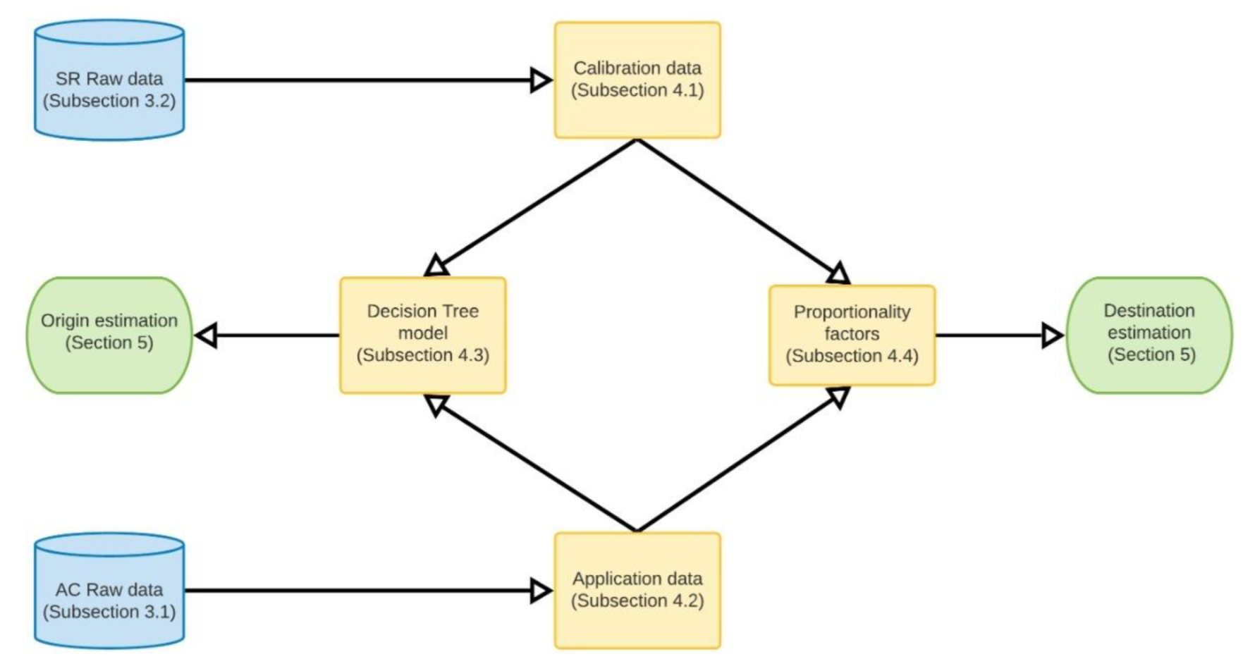
The contribution of this article is twofold. First, we proposed a methodology to estimate the origin of all the trucks traveling on an urban highway. The methodology involved the calibration of a decision tree model using biased GPS data from the routing company we worked with, which was complemented with freight companies’ data from Chile’s Internal Revenue Service. Then, this model was applied to data gathered from free-flow toll gates equipped with Automatic Vehicle Identification (AVI) technology in order to determine the origin of those trips. Second, we estimated the destinations of all the trucks traveling on the highway. To do so, we computed proportionality factors using the trips built from the GPS data, based on the origin municipality. The use of complementary information (AVI and GPS) and decision trees allowed us to mitigate the bias of OD estimation. We believe that the methodology proposed in this research is replicable in other contexts outside Chile, since license plate tracking technology is standard on highways in several countries worldwide, mainly to collect tolls or detect stolen vehicles. Additionally, the methodology requires GPS tracking information from only a subset of the total number of freight vehicles and readily available freight company-related information.

The rest of this article is organized as follows. Section 2 reviews the literature. Section 3 describes the data used in this article. In Section 4, the methodology used to obtain the OD matrix is presented, while Section 5 applies this methodology to the case of Autopista Central. Finally, in Section 6, we provide some final remarks, and we conclude by highlighting lines for future research.

2. Literature Review

This section reviews the literature on freight OD matrix estimation. We divide our literature review into two subsections according to the use of active and passive data, respectively.

2.1. Active Data

Active data collection indicates that data is generated by involved and sporadic user input [24]. Among this type of data, the most used are surveys, i.e., questionnaires that seek to obtain information directly from the source. These can be primary or secondary, which means they can be taken directly by the researcher or an external agency.

Several articles in the literature use this type of data. For example, Muñuzuri et al. [14] uses retailer surveys as a primary source of information and data from governmental organizations in the city of Seville, Spain, as secondary information. Through an entropy-maximization model, the authors use both sources of information to estimate six OD matrices for delivery to retailers and home delivery. The results are then validated with traffic-count data collected in specific city areas.

Al-Battaineh and Kaysi [15] uses flow data obtained by the Ministry of Transportation of Ontario, Canada, through surveys of commercial vehicles. This information is complemented with field data obtained by the Canadian statistical office. From this data, attraction (destinations) and production (origins) zones are identified, adjusting the flow data obtained in these zones through an optimization model that is solved using a genetic algorithm. Holguin-Veras and Patil [16] considers data in Guatemala City gathered from primary sources, including vehicle type, origins and destinations, types of products transported, and other information. This data is complemented with traffic counts. The authors combine a gravity demand model of commodity flows and a complementary model of empty trips, and obtaining that the latter’s inclusion significantly improves the OD matrices’ estimation.

Muñuzuri et al. [11] also estimates the OD matrix but focuses on a business-to-business model for retailers in Seville, Spain. The authors use data from retailer surveys, which provides information on frequencies, quantity, duration, and type of vehicle used in the delivery, among other data. This data is used to formulate a trip-generation model and an assignment model that maximizes the entropy. Then, this model is compared against a classical gravity model using traffic count data in selected areas. The authors show that the proposed model outperforms the gravity model even though the former estimates the OD matrix with more limited information.

Finally, Nuzzolo et al. [12] uses surveys of freight vehicle drivers to obtain information related to the load, the delivery, the stops made, and drivers’ personal information. The authors calculate the number of stops per route and estimate the sequence of deliveries during a trip. The model system allows computing freight OD matrices.

2.2. Passive Data

Passive data corresponds to information collected using inbuilt sensor technologies [24]. Unlike active data, passive data shows a much higher application potential as it has a lower collection cost and a high update frequency.

Ma et al. [19] uses data from multiple sources, including automated license plate recognition, Bluetooth, and GPS, to estimate an OD matrix in a specific section of a road linking a port in Rotterdam, the Netherlands, with different distribution centers in Germany. The authors propose the joint use of two models: a Bayesian Network model and an entropy-maximization model.

Gingerich et al. [21] uses GPS data corresponding to commercial vehicles that entered the United States from Canada over two specific bridges in 2013. First, the authors develop a methodology that allows trip identification from this data, differentiating intermediate stops and final stops. Then, the OD matrix is estimated, making it possible to analyze freight generation and demand. In Chankaew et al. [22], heavy vehicle GPS data is obtained in Thailand. This data is complemented with road traffic count data to estimate trip origins and destinations by the maximum likelihood method.

In some countries, there are some private and public institutions that seek to gather and centralize freight information. An example of this is The American Transport Research Institute (ATRI), a governmental institution in charge of collecting freight data by encouraging this information exchange between private parties in the United States, making it possible to conduct transportation studies. For example, in Bernardin et al. [18], ATRI data sources are used to construct an OD matrix, subsequently employed to improve travel demand estimation in Indiana, EEUU.

Elsewhere, Zanjani et al. [20] uses GPS and traffic count data in Florida, EEUU. The authors estimate freight OD matrices using an optimization model, minimizing the difference between the estimated and observed flows. Kuppam et al. [25] uses ATRI data in Arizona. First, the raw GPS data is used to generate trips with their respective intermediate stops. A model is then used to estimate logistics indicators, including the total number of trips per zone and the number of visits on each trip.

The works developed by Bernardin et al. [18], Kuppam et al. [25], and Zanjani et al. [20] consider a sample representing a significant percentage of total trips. For example, in Zanjani et al. [20], this percentage reaches 10%. These values can be explained by the existence of institutions such as ATRI that encourage the exchange of information between private parties. However, to the best of our knowledge, this type of initiative does not exist in most other countries. Therefore, the development and use of methodologies to estimate OD matrices must deal with a small and less representative data sample. Our research seeks to help bridge this gap.

3. Raw Data Description

We use two passive data sources to estimate a freight OD matrix in Santiago, Chile: Autopista Central toll gates data and SR routing data. The considered period was July 2019. We complement these data sources with the economic sector of the companies that are customers of SR and the economic sector of the trucks that use Autopista Central. For this purpose, we use information from Chile’s Internal Revenue Service, which assigns one primary economic sector to all companies according to the activities declared in their income operations.

3.1. Autopista Central Data

The first source of data is the information obtained from the free flow toll gates of Autopista Central, one of the most important highways within the city of Santiago. This highway is over 60 km long, crossing 10 of the 34 municipalities of the metropolitan area of Santiago on its General Velásquez and North/South axes, as shown in Figure 1. This highway has 31 free-flow electronic toll gates equipped with automatic vehicle identification (AVI) technology, which provides vehicle-by-vehicle information. In particular, for each vehicle crossing each gate, the data includes the lane, the speed, the time, the license plate, and the category (light cars, motorcycles, or heavy vehicles). This information is obtained through TAG devices, which are electronic instruments installed on the front windshield of vehicles. All vehicles that use the highway are forced by law to have a TAG.

Table 1. Variables contained in the AC raw database.

Variable	Description
Timestamp	Date and time a vehicle passes through the gate.
Speed	Speed (in km/h) at which the vehicle passes.
Category	Vehicle category.
License plate	Vehicle license plate.
Gate	Gate number through which the vehicle passes.
Lane	Lane number on which the vehicle passes (1 to 3, right to left).

shows the information contained in each observation of the database. On the other hand,

Table 2. Distribution of license plates and observations in AC database.

Category	Number of License Plates	Percentage of License Plates	Number of Observations	Percentage
Light vehicles	1,520,171	90.87%	43,293,570	85.72%
Heavy vehicles	133,570	7.98%	6,497,911	12.87%
Motorcycles	19,255	1.15%	708,779	1.41%

shows the distribution of the number of license plates and observations for each category using the highway in July 2019.

Overall, 50,503,009 vehicles passed through the toll collection gates during July 2019. Only heavy vehicles were considered for this research, which led us to 6,497,911 observations. From these observations, we eliminated those heavy vehicles providing passenger transportation services using the license plate data. Subsequently, private heavy vehicles were also excluded using Chile’s Internal Revenue Service information. In other words, this work was restricted to trips made by company-owned vehicles. After all this filtering, the considered database consisted of 3,751,553 observations. For this dataset, Figure 2 shows the number of observations according to the gate, while

Table 3. Summary of AC heavy vehicles database.

Number of License Plates	61,763
Average daily number of gates passed through by each vehicle	7.30
Daily average of vehicles	7644.69

shows a statistical summary.

3.2. SimpliRoute Data

The second source corresponded to information gathered during July 2019 by SR through the service it provides to its customers. Each customer informs SR of the visits to be made, the vehicles, and the available drivers. SR, in turn, suggests a route to follow according to the objectives the client prioritizes.

Table 4. General overview of SR data during July 2019.

Total Number of Routes	24,149
Total number of visiting points	1,218,800
Total number of GPS pings	19,501,223

shows general information regarding the number of routes, visits, and GPS during the studied period, whereas

Table 5. Descriptive analysis of SR customers.

	Routes	Visits	Visits Per Route
Number of customers	Daily average per customer (SD)	Daily average per customer (SD)	Daily average per customer (SD)
154	9.9 (13.2)	467.3 (1703.1)	46.5 (88.2)

presents a descriptive analysis of SR customers’ planned routes and stops. In what follows, we refer indistinctly to a trip or route.

SR had 154 customers registered in the databases, with 2223 different vehicles routed. The tracking of these vehicles on the road was done through the onboard GPS. In the case of vehicles without GPS, SR performed GPS tracking through the cell phone.

Table 6. Descriptive analysis of SR’s tracking database.

Average time (SD) between pings in seconds	47.32 (178.47)
Average (SD) number of vehicles per client	11.65 (26.07)
Average (SD) number of pings per day per vehicle	786.59 (1044.07)

provides more specific GPS information.

4. Methodology

This section presents the methodology used for the estimation of the OD matrix. For the sake of exposition, the methodology’s presentation is done using the SR and AC data. However, the proposed methodology can be employed using other biased GPS tracking data and license plate recognition data from an urban highway. Figure 3 depicts a diagram of the proposed methodology, indicating the corresponding manuscript section in which the procedure was developed.

4.1. From SR Raw Data to Model’s Input Variables

The GPS data provided by SR allowed us to track the movement of the trucks that followed the planned route each day. Each of the planned routes had an origin and multiple visits and was carried out by a specific vehicle and driver from each one of the SR customers. Using the GPS data, it was possible to rebuild the trajectory of each vehicle on the road by grouping the GPS data associated with each vehicle or driver on a specific day. This is depicted in Figure 4.

For determining the origin, we assumed that the first ping of the day corresponded to the start of the vehicle’s trip. Then, to determine when a vehicle was on Autopista Central, we used a decision rule based on the distance from the GPS ping to the highway. Specifically, we considered that a truck was on the highway when this distance was below a 100 m threshold. We then identified the route sections covered by each vehicle using the highway. We considered only trips in which at least three consecutive pings have been recorded in the highway according to the 100 m rule. This helped reduce misclassification of the vehicles that used close local roads. Additionally, since this research focused on identifying the load-generating points, the analysis was restricted to the first of the route segments that used the highway during each day.

Subsequently, for each of the highway trips considered, the entry AVI gate was identified. We assumed that this gate was the one closest to the starting point in the direction of the vehicle’s movement. Similarly, the exit AVI gate was identified as the one closest to the ending point. Figure 5 shows an example of the GPS pings of a vehicle in the proximity of the highway. The blue points correspond to those identified as off the highway, while the purple points are those identified as on the highway. In this example, the green mark is the starting gate of that section on the highway, considering the rules explained above.

With the information for each first segment of the day, we generated the input variables used to train the decision tree model employed for origin estimation. These variables are shown in

Table 7. Input variables for the model.

Variable	Description
Municipality of Origin	The municipality of origin of the trip (dependent variable)
Start time	The time the vehicle enters the highway
Journey time	The journey time between the first and last gates
Distance covered	The distance covered using the highway
Gate of entry	The first gate crossed
Gate of exit	The last gate crossed
Sector	The economic sector associated with the client making the trip

. The municipality of origin of the trip was the dependent variable, while the others were the independent variables.

4.2. From AC Raw Data to Model’s Input Variables

To apply the model described in the following subsection, we had to transform the AVI gates’ data (Section 3.1) into vehicle trips’ data in order to generate a base analogous to that of SR (Table 7). To recognize trips, we had to identify when two consecutive AVI detections of the same license plate corresponded to the same journey. For this purpose, we used the methodology proposed in Basso et al. [27], consisting of two simple rules. The first rule indicates that if the crossed AVI gates are not contiguous in the direction of movement, then the vehicle must have left the highway for this to occur. On the other hand, the second rule involves a lower limit (5 km/h) for the speed a vehicle can travel on the road. Mathematically, if the constraint shown in Equation (1) is satisfied, then we assume that both AVI detections correspond to separate trips, where $D$ corresponds to the distance (in km) between the two contiguous AVI gates and $T$ to the time between them (in seconds).

$$3600\times \frac{D}{T}<5$$

(1)

Two AVI gate detections for the same license plate belong to the same trip if they do not meet the two rules mentioned above. Once all the AVI gate detections of a trip were identified, we computed the rest of the variables shown in Table 7, except for the unknown municipality variable. Additionally, in this case, the economic sector was obtained by identifying the company’s name that owned the vehicle through the license plate.

4.3. Estimating the Trip’s Origin Using Decision Trees

Since there is no accurate data in Chile to contrast the OD estimates, one way to validate the proposed procedure is through experts’ criteria. For this reason, in addition to obtaining the classifications’ results, we also had to consider the interpretability of the model. Because of this, we followed a decision tree approach. Unlike other machine learning models, the decision trees methodology is interpretable, for example, in terms of variable relevance [28].

Following Mohri et al. [29], we now present a general overview of decision trees. A decision tree starts the classification through a root node, the label of which corresponds to the category with the highest frequency within the dataset. This node is divided into two disjoint subsets, depending on the result of a binary logical test related to one of the model’s input variables. The labels of the resulting two nodes correspond to the category with the highest frequency within each subset. There are different types of methods to train the model based on the gaining of information at each new node. One of these is the so-called greedy method, which seeks to minimize the impurity at each node according to a measure given by the formula presented in Equation (2) [29]:

$$\widehat{F}\left(n,q\right)=F\left(n\right)-\left[\eta \left(n,q\right)\times F\left(n_{-}\left(n,q\right)\right)+\left(1-\eta \left(n,q\right)\right)\times F\left(n_{+}\left(n,q\right)\right)\right]$$

(2)

where $\widehat{F}\left(n,q\right)$ corresponds to the decrease in impurity at node $n$ when using test $q$, while $n_{-}\left(n,q\right)$ and $n_{+}\left(n,q\right)$ are the corresponding left and right leaves, respectively. $\eta \left(n,q\right)$ corresponds to the proportion of observations remaining on the left leaf after splitting node $n$ with test $q$. Finally, the function $F$ corresponds to a predefined impurity measure (e.g., misclassification, entropy, and Gini index). Finally, it is possible to define a measurement of importance of the input variables used. This importance is defined as the total decrease in the aforementioned impurity over the total number of times the variable in question is used in the model. Once the model is trained, it can be used for prediction purposes.

Let us define $J$ as the set of municipalities, $S$ as the set of economic sectors, and $I_s$ as the set of trips for vehicles owned by companies of the economic sector $s \in S$. Since the objective of this research was not to study individual freight trips, but to estimate an aggregate measurement of freight movement, the outcome of the model was used as a vector of probabilities $P_{ij}$, which corresponded to the probability predicted by the model that trip $i \in I_s$ originates at municipality $j \in J.$ Using these definition, Equation (3) defines the estimate of the number of trips $O_{js}$ that start in municipality $j \in J$ for economic sector $s \in S$. Summing over the economic sectors $s \in S$, we obtained the estimated total number of trips starting at municipality $j \in J$, as shown in Equation (4).

$$O_{js}={\displaystyle \sum }_{i \in I_s}^{}{P}_{ij} \forall j \in J, s \in S$$

(3)

$$O_j={\displaystyle \sum }_{s \in S}^{}{O}_{js} \forall j \in J$$

(4)

4.4. Estimating the Trip’s Destinations Using Proportionality Factors

We estimated the trip’s destinations using a proportional method. For each trip within the AC database whose origin was municipality $j \in J$, we supposed that a number of ${\delta }_{jk }$ stops (destinations) occurred at municipality $k \in J$. This number was estimated according to Equation (5) considering the data in the SR database, where $V_{jk}$ corresponds to the trips whose origin is municipality $j \in J$ and one of its destinations is $k \in J$, respectively, whereas $N_j$ corresponds to the total number of trips starting at municipality $j \in J$.

$${\delta }_{jk }=\frac{V_{jk}}{N_j}, \forall j,k \in J.$$

(5)

Therefore, the proportionality factor is ${\delta }_{jk }$ is the conditional expectation of the number of stops that a trip has in municipality $k \in J$ given that the trip starts in municipality $j \in J$. Note that ${\delta }_{jk }$ combines two effects: (i) the expected number of stops for each trip, conditional in $j \in J$, and (ii) the probability that each one of these stops occurs in municipality $k$.

An estimation of the number of trips $T_{jk}$ that start in municipality $j \in J$ and end in municipality $k \in J$, is given by Equation (6).

$$T_{jk}=O_j\times {\delta }_{jk} \forall j,k \in J.$$

(6)

Finally, Equation (7) defines the estimate of the number of trips $D_j$ that end in municipality $j \in J$, which, along with $O_j$, allowed us to estimate the OD matrix.

$$D_j={\displaystyle \sum }_{k \in J_{}}^{}{T}_{jk} \forall j\in J.$$

(7)

5. Results

We considered initially the 19,501,223 GPS pings corresponding to the movement of SR vehicles during July 2019. Following the methodology described in Section 4.1, we identified 570,696 GPS pings on the highway, which led to 12,097 trips that used the highway. Subsequently, by considering only the first segment of the day for each vehicle, this dataset was reduced to 5190 trips that used the highway. 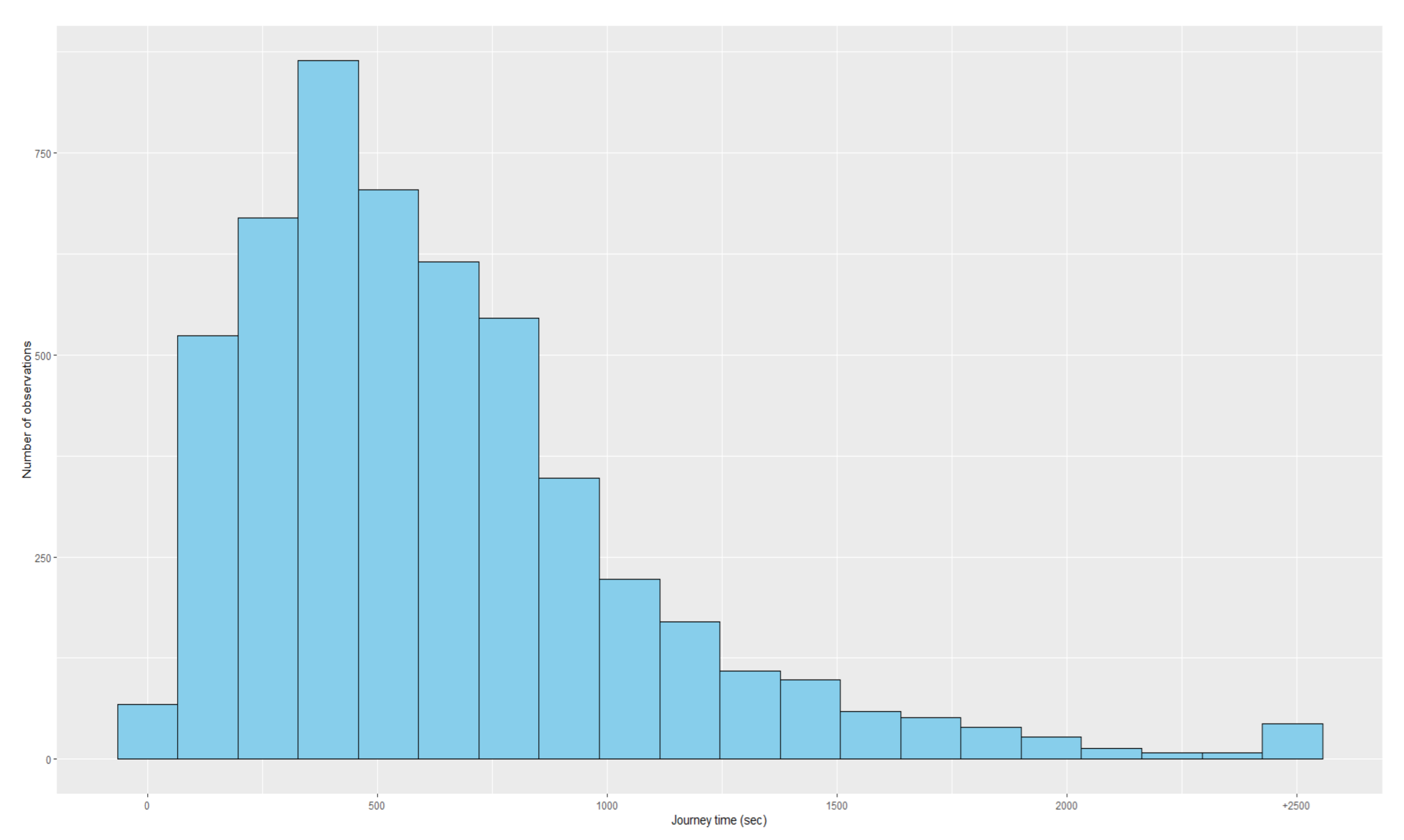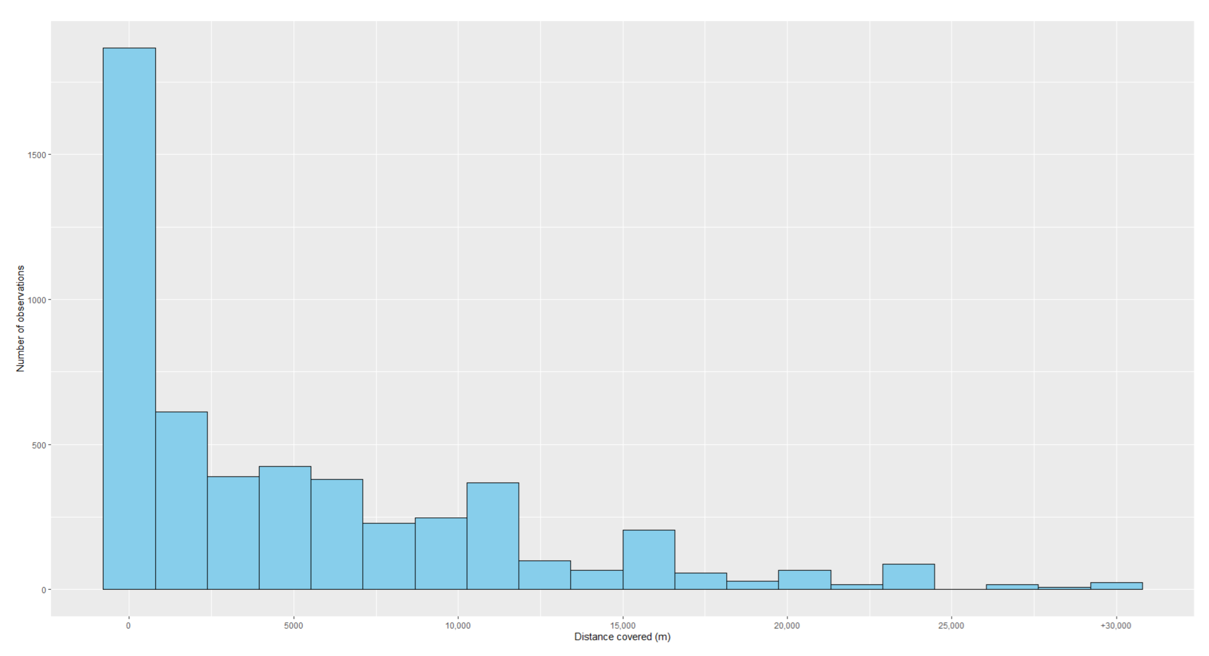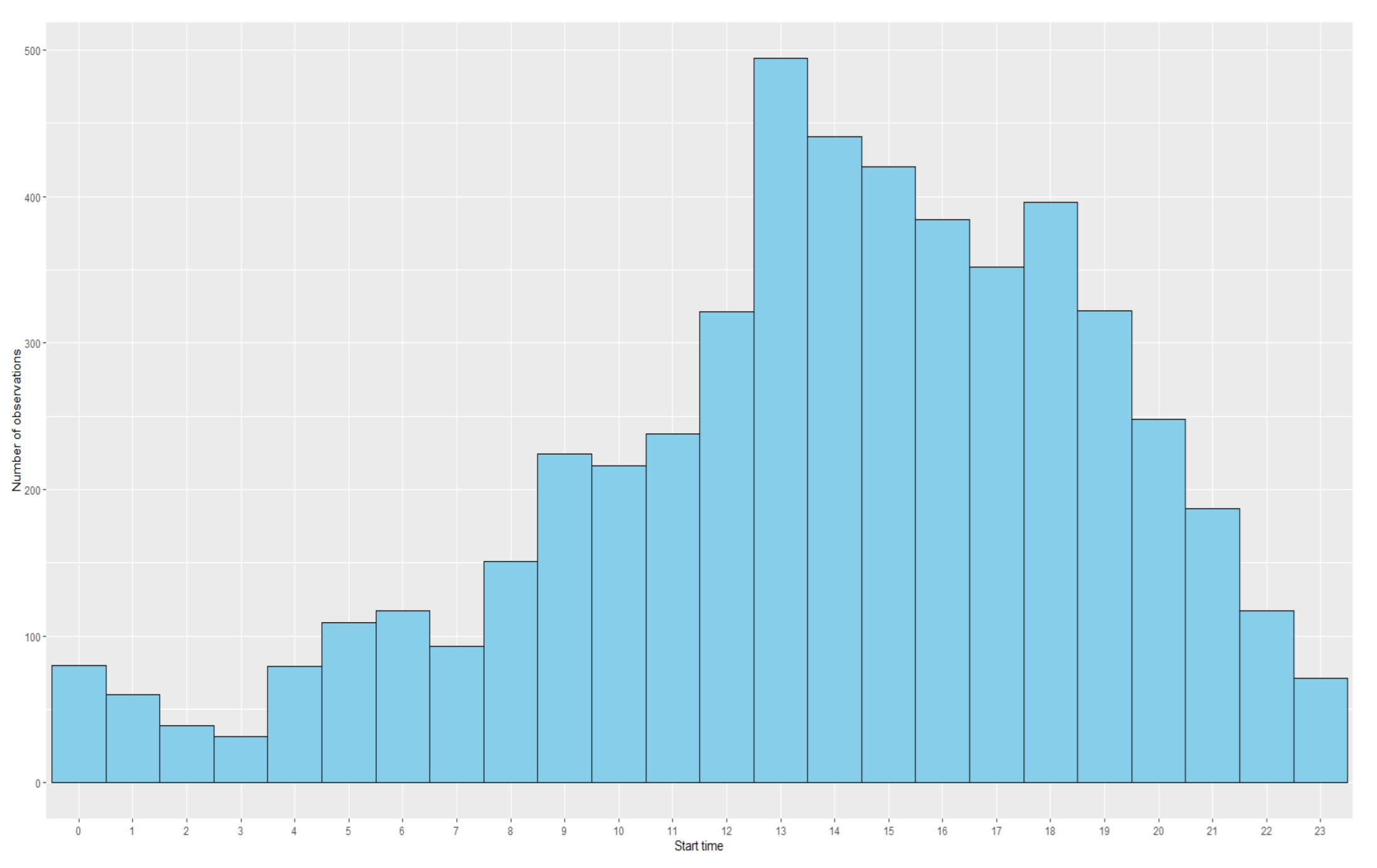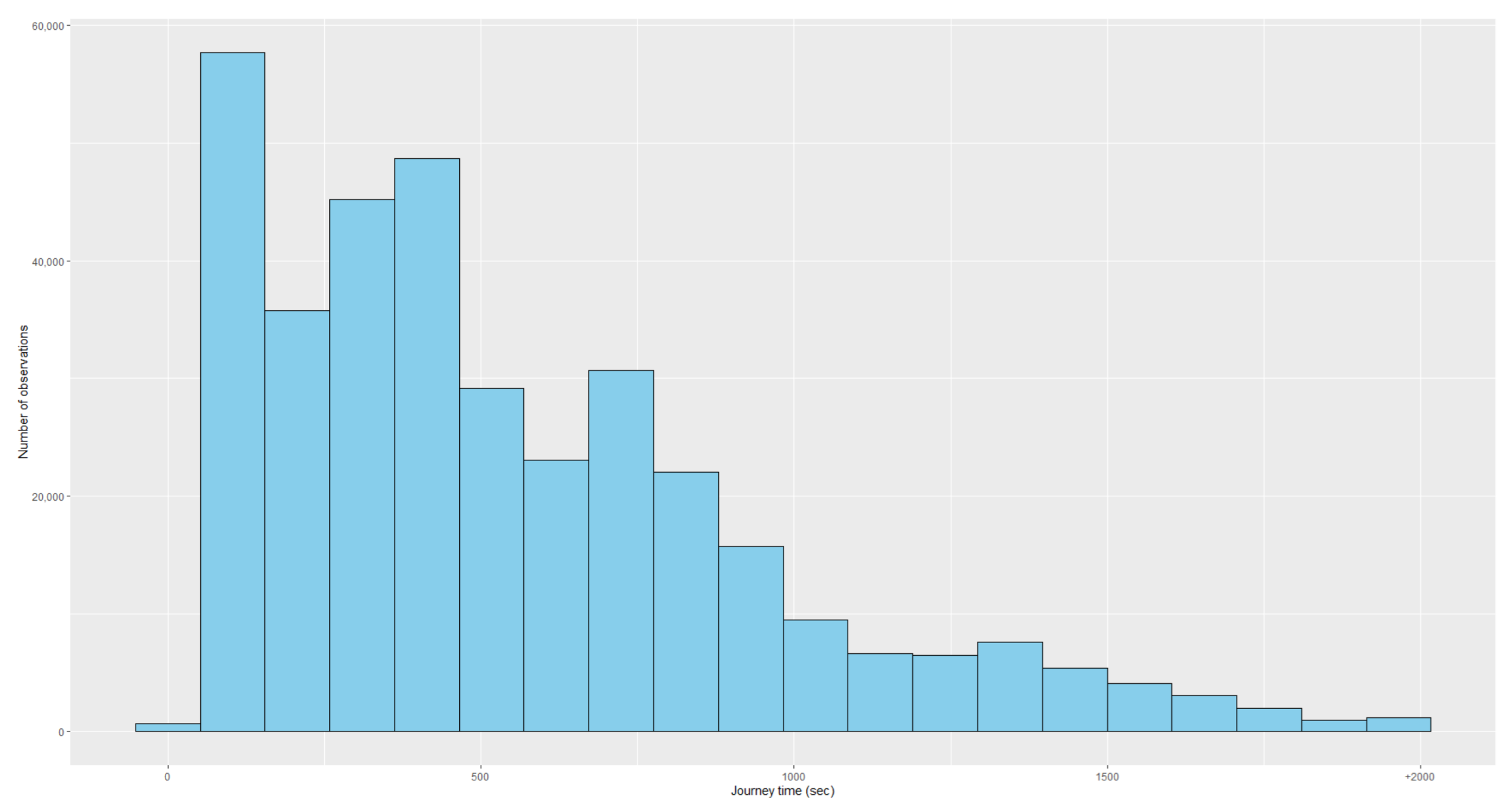For each of these trips, we generated the variables shown in Table 7. A descriptive analysis of these variables is presented in

Table 8. Descriptive statistics of input variables.

Variables	Mean (SD)	Mode (Number of Repetitions)
Journey time (s)	656.16 (777.57)	360 (24)
Distance covered (m)	8895.43 (6817.1)	0 (1866)
Start time	13.8 (5.06)	13:00 (494)
Gate of entry	-	Gate 15 (524)
Gate of exit	-	Gate 7 (573)
Economic sector	-	H (2185)

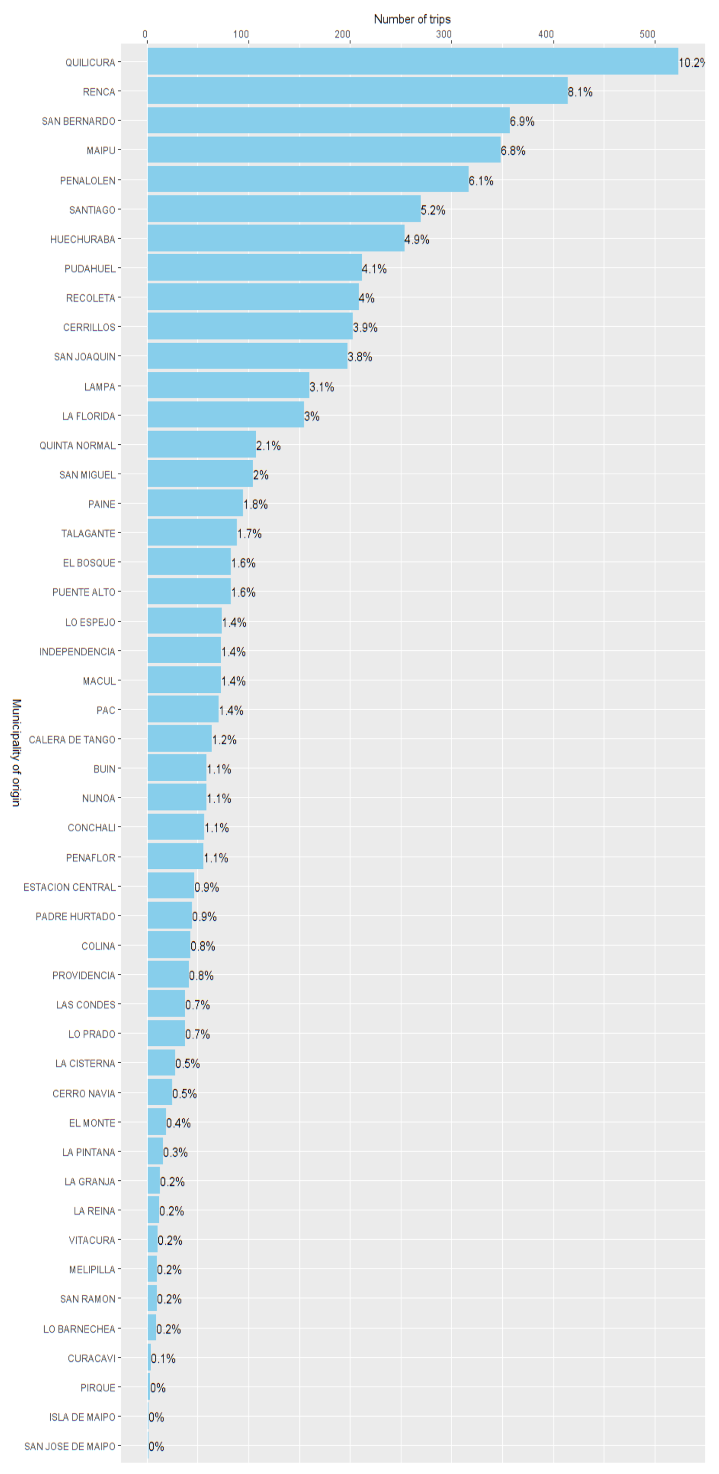
, while histograms of the numeric variables can be found in Figure A1, Figure A2 and Figure A3 in the Appendix A. Figure 6 shows the distribution of trip origins, which provides the first insights into the AC’s freight trips.

After the SR final dataset was constructed, we trained the decision tree described in Section 4.3. First, to assess the model’s performance, we adopted a training validation approach. In particular, we trained the model on a random subset of 4512 observations (80%), pruning the tree at the level that reached the minimum error on this training base. Then, we used this model to predict the remaining 1038 observations (20%). Using 80% of the sample to train statistical learning models and using the remaining 20% to validate it is a common practice (e.g., [30,31,32]). Using more balanced training and validation datasets sizes (e.g., 50%–50%) has the disadvantage of reducing the training set size, and consequently, increasing the trained model variance [33]. This, coupled with decision trees being high-variance methods [34], can lead to unreliable estimates.

With this approach, we obtained a validation mean absolute percentage validation error (MAPE) of 14.5%. This error was in line with results reported in the literature for similar contexts, for example, passenger origin–destination estimates using statistical learning methods. For instance, using a probabilistic model, Dai et al. [35] reports an average MAPE of 13.26% for subway short-term passenger inflow in Zhengzhou City, China. Similarly, using convolutional neural networks, Yao et al. [36] shows that its best-performing model presents a MAPE of 24.3% for taxi flows in Beijing, China.

We then adjusted the decision tree model using the complete SR final database. After pruning the tree at the lowest training error level, we obtained a tree of 44 levels.

Table 9. Importance of the input variables.

Variable	Importance
Start time	623.32
Journey time	375.74
Distance covered	313.88
Gate of entry	661.77
Gate of exit	578.33
Economic sector	267.75

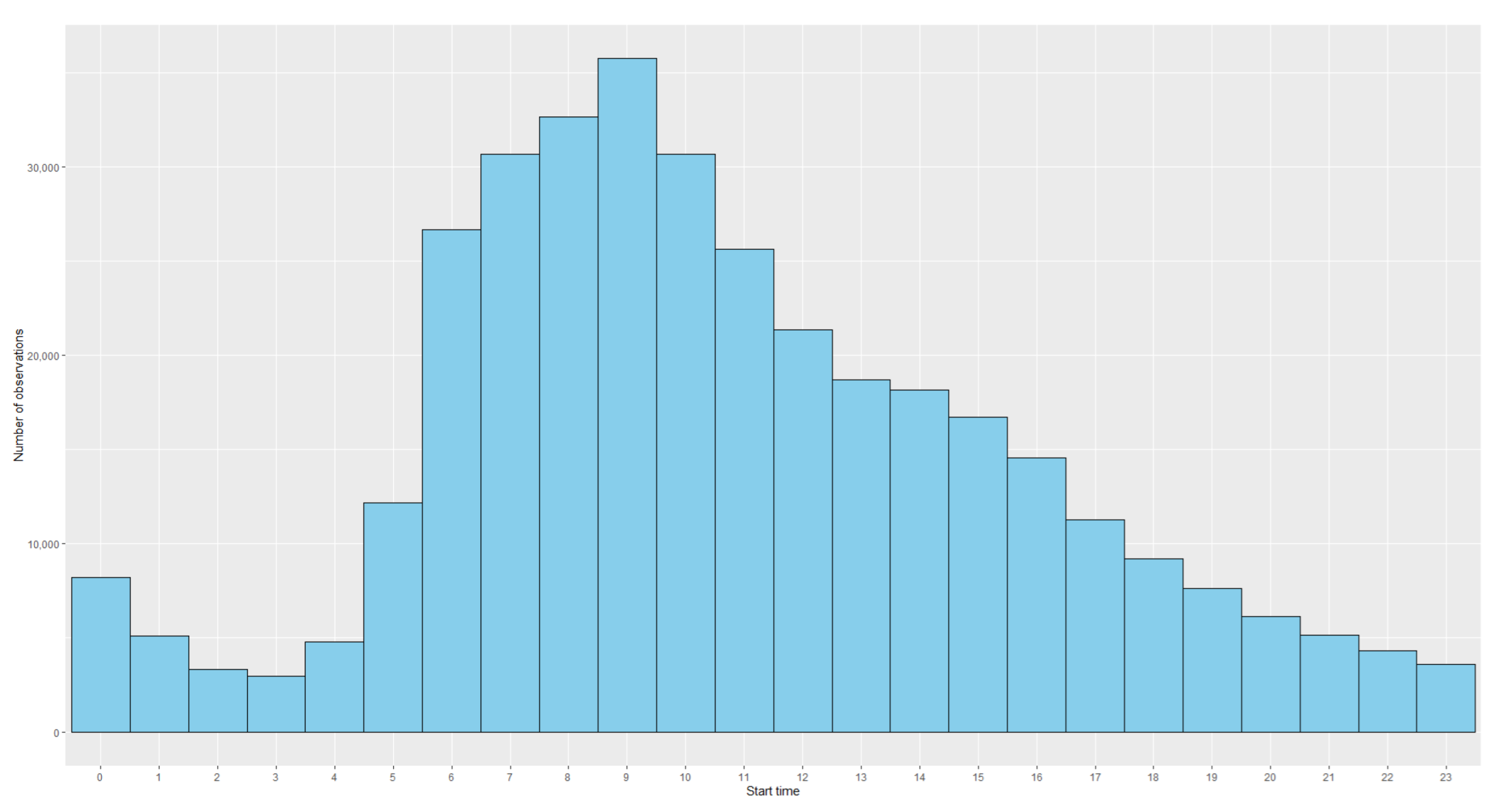
shows the variable importance in the tree, as described in Section 4.3. The gate of entry was the variable with the highest importance since, intuitively, it tended to be the one most correlated with the start of the trip. Likewise, note that the start time was also a high-importance variable. From this, we could imply that, depending on the municipality, trips started at significantly different times. Conversely, the economic sector was the least important variable for the decision tree. Therefore, the trip start municipality was not significantly influenced by the economic sector of the vehicle owner company.

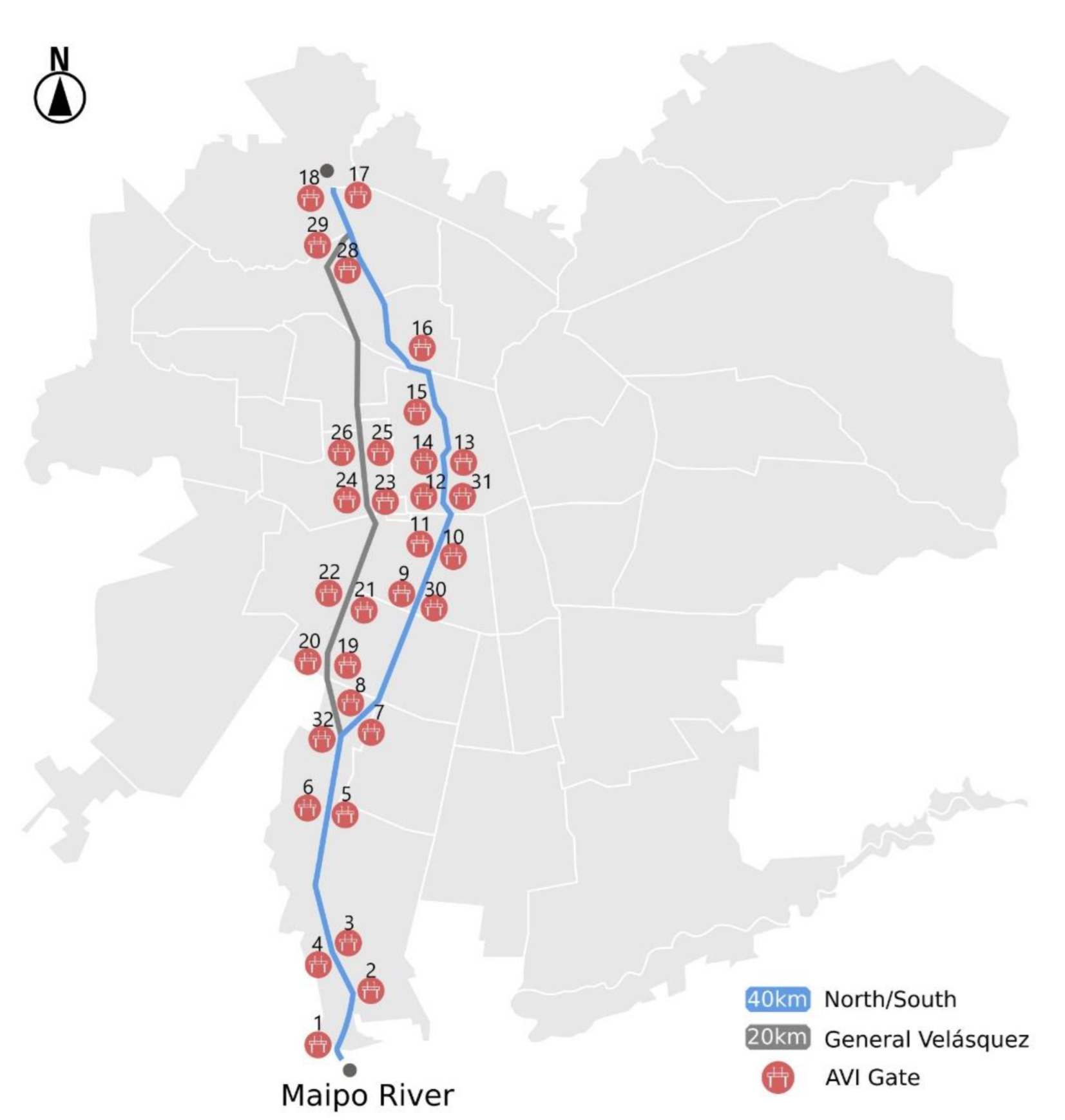
Afterward, the AC database was generated following Section 4.2. To do so, we considered the 3,751,553 AVI gate observations during July 2019. From this, we constructed 759,576 AC trips. This dataset was reduced to 355,400 trips by considering the day’s first trip for each license plate only.

Table 10. Descriptive statistics of AC variables.

Variables	Mean (SD)	Mode (Number of Observations)
Journey time (s)	547.25 (398.75)	111 (1024)
Distance covered (m)	11,344.11 (8309.87)	10,750.61 (19,267)
Start time	10.67 (4.89)	09:00 (35,738)
Gate of entry	-	Gate 2 (69,091)
Gate of exit	-	Gate 17 (61,098)
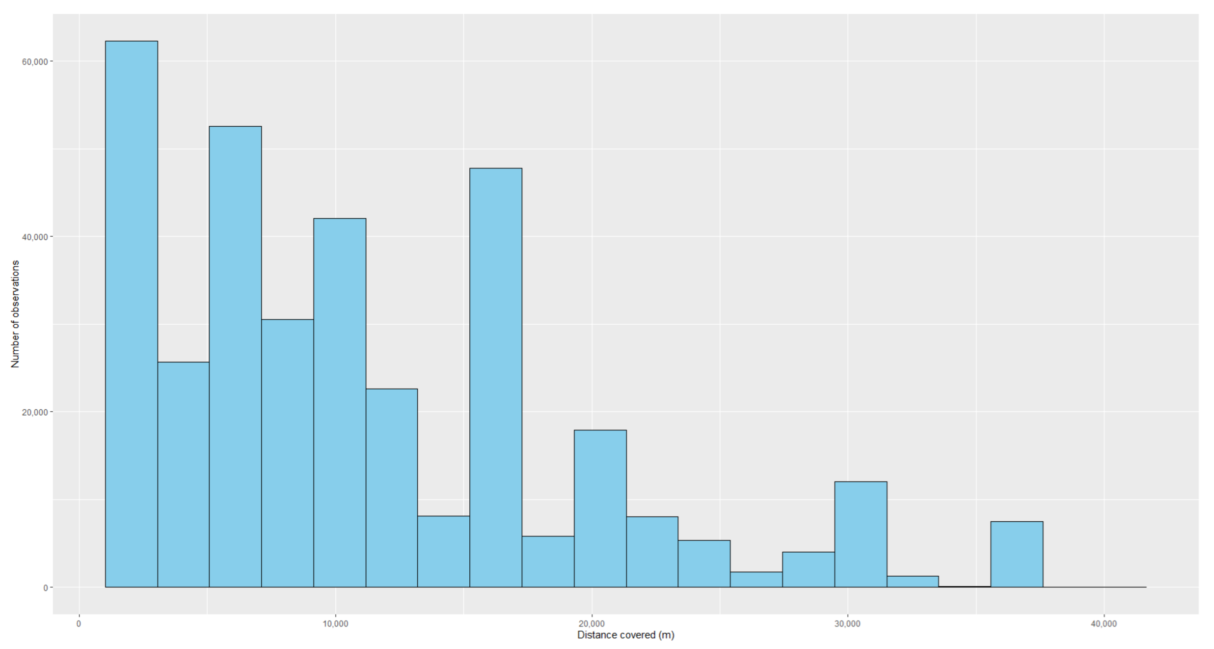
Economic sector	-	J (111,339)

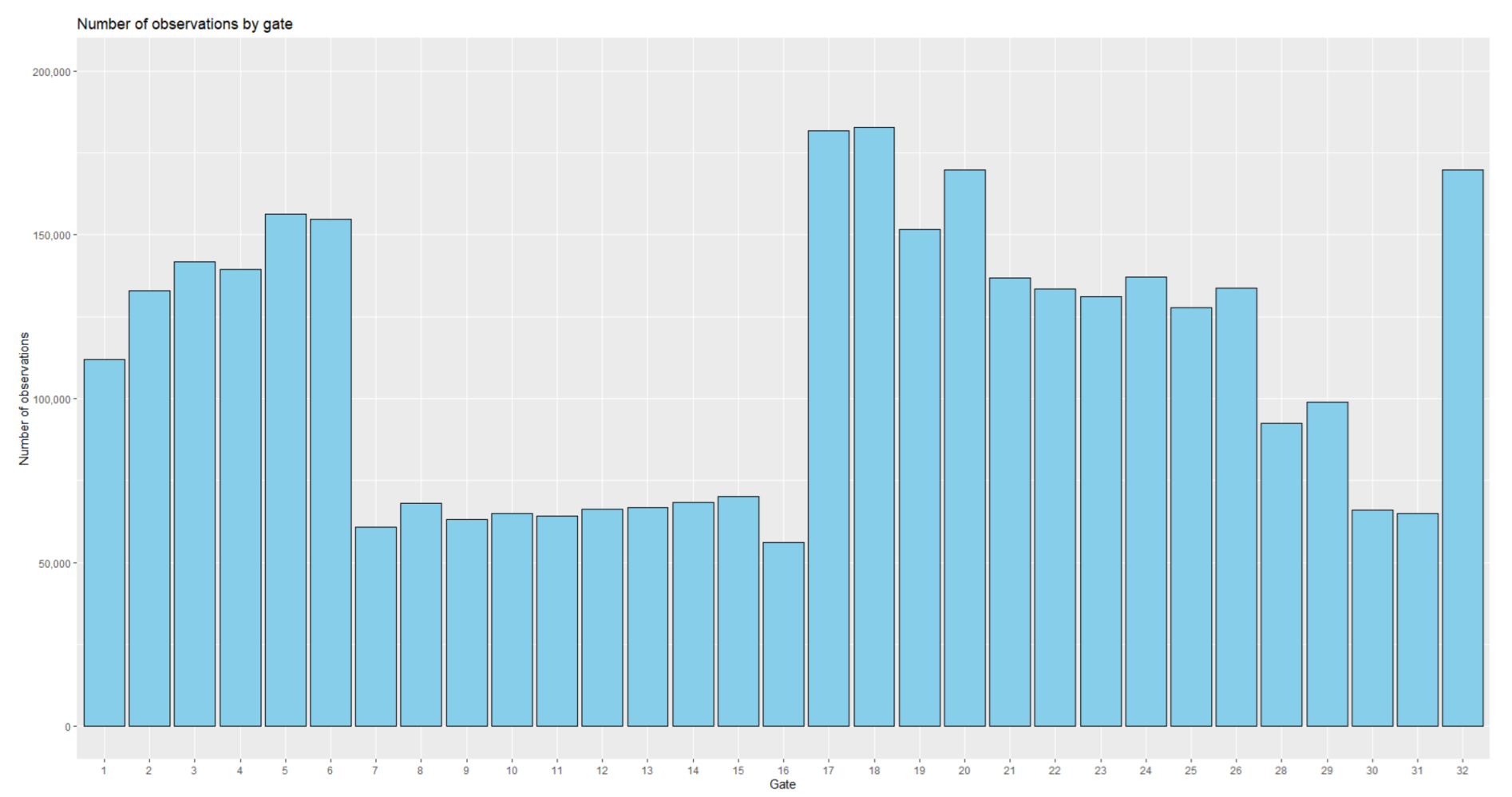
shows a descriptive analysis of the variables associated with these trips, while histograms of the numeric variables can be found in Figure A4, Figure A5 and Figure A6 in the Appendix A. Figure 7 shows the distribution of the number of trips depending on the entry gate’s municipality. This distribution provided further insights into the AC’s freight trip origins.

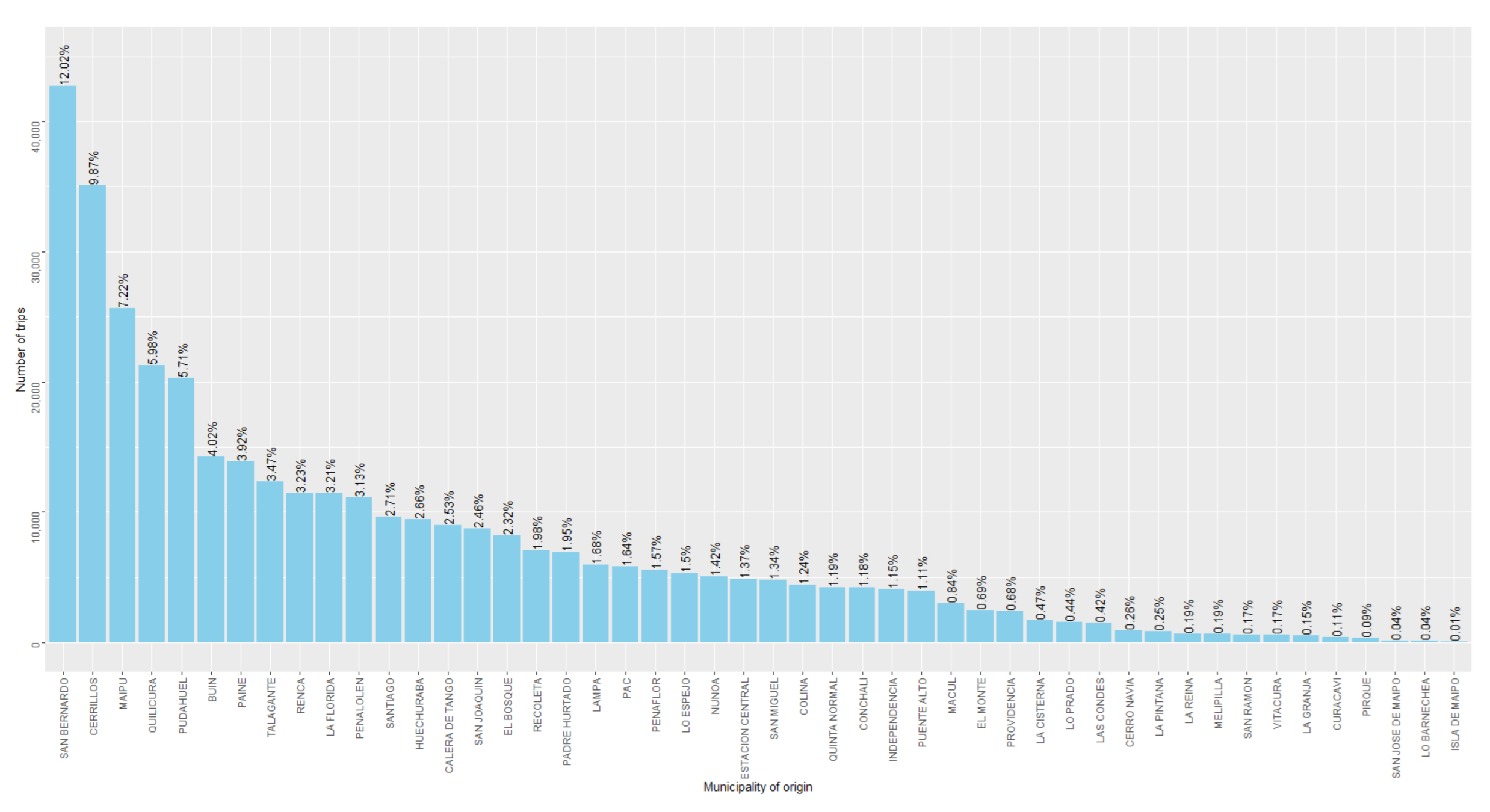
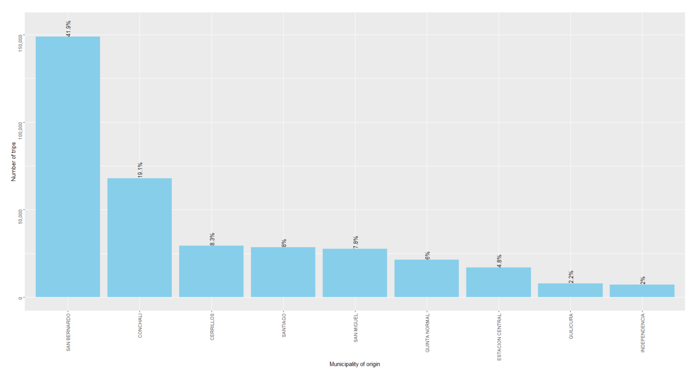
Once the AC database was obtained, the decision tree previously trained in the complete SR base was applied to the observations obtained from AC, calculating the values of $O_{js}$ for all the municipalities j ∈ J and economic sectors s ∈ S following Equation (3). Using Equation (4), summing over the economic sectors s ∈ S, we obtained the number of trips $O_j$ starting at each municipality j ∈ J. The distribution of the estimated trips per origin is depicted in Figure 8.

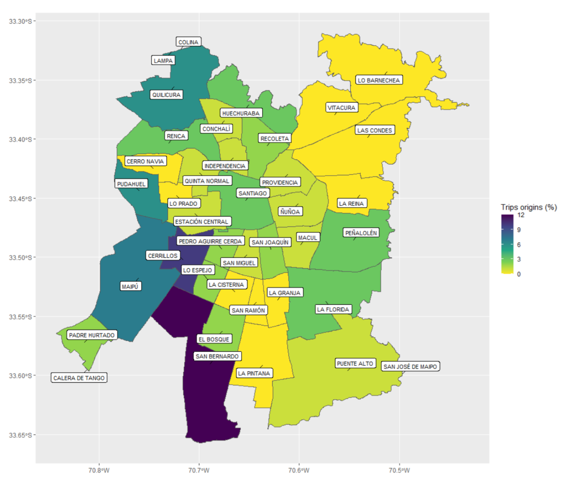
Figure 9 and Figure 10 present the distribution maps of trip origins and destinations per municipality, respectively. From Figure 9, we could see that most of the trips started on the westernmost outskirts. The suburbanization of warehousing is an increasingly common phenomenon in cities [37], and it has been termed as “Logistics Sprawl” [38]. Indeed, for example, in most US cities, freight distribution activity has moved from its traditional central city locations to suburban in the last decades [39]. The main reason for this shift is the increase in land prices in central areas, combined with both the availability of affordable land and connections to transport infrastructure in suburban locations [40]. This last is indeed the case of Santiago, where the westernmost municipalities provide at the same time some of the lowest land prices and connections to the largest urban highways and the two most important ports in the country, Valparaíso and San Antonio.

This pattern of freight trips brings multiple challenges to cities. For example, more distant terminals increase the freight transport total mileage since central locations—the main destinations of the trips—lack affordable and available land to locate logistics facilities [38]. This, in turn, increases both congestion and total emissions generated by logistics activities [41]. In this regard, different measures and policies have been proposed to make urban logistics more sustainable. For instance, some authors argue that local authorities should evaluate the benefits of easing the presence of logistics facilities in the inner city to reduce travel distances (e.g., [42]), while other authors have shown that freight time restrictions can help alleviate the negative effects of logistics sprawl [43].

As in most countries, there is no public data in Chile to validate these results. For this reason, we proposed a validation based on land use information provided by Chile’s Internal Revenue Service. This method establishes the total square meters destined for commercial land use for each municipality. Subsequently, we computed the Pearson correlation between such land use and the proportion of trips by origin obtained according to (i) original distribution of SR data (Figure 6), (ii) distribution according to the municipality of the gate of entry of the trip (Figure 7), and (iii) the distribution predicted by our approach (Figure 8). These correlations were 0.504, −0.501, and 0.548, respectively. Thus, our approach maximized the mentioned correlation. This suggests that our OD matrix could better represent the distribution of commercial activities in the city, compared to the other two simpler approaches, by mitigating the bias of the GPS data.

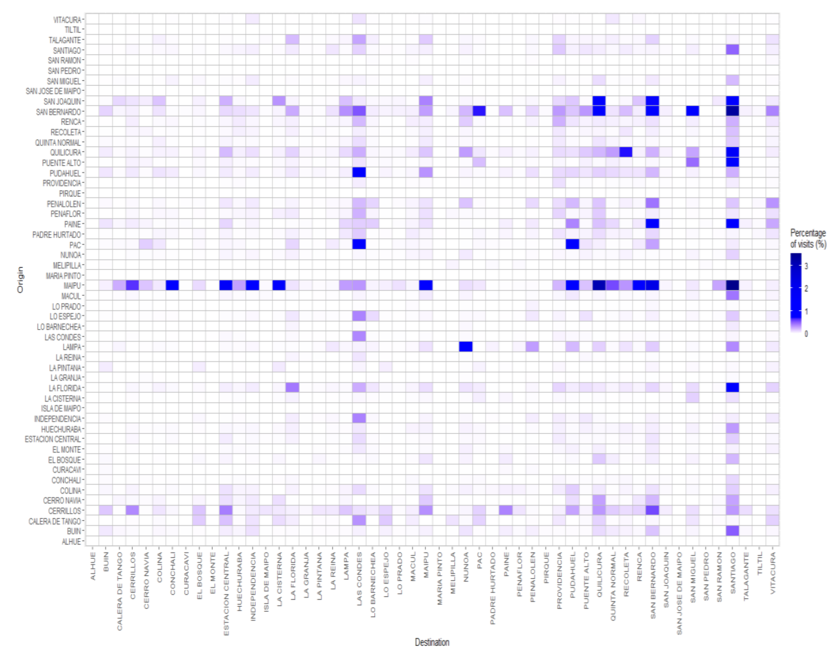
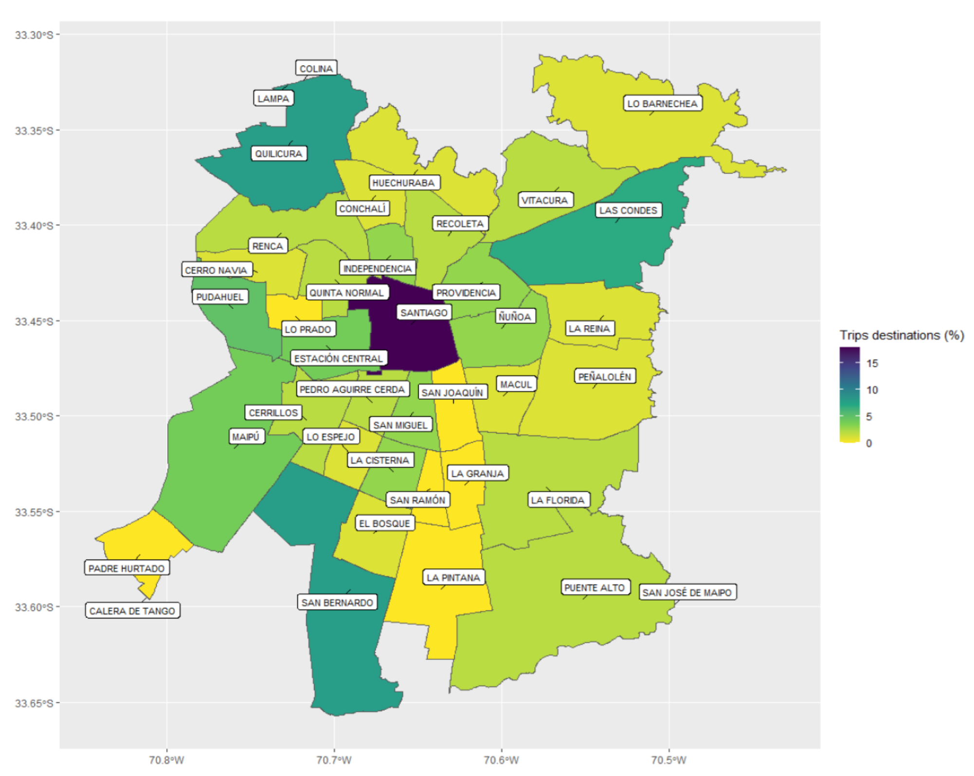
Finally, using Equations (5) and (6), we estimated the entries $T_{jk}$ of the estimated OD matrix. Figure 11 shows these results as percentages of the overall estimated visits.

6. Discussion and Conclusions

Freight transportation can generate several negative externalities such as pollution, congestion, and wear and tear on infrastructure. These externalities negatively impact the urban environment [44]. Thus, it becomes relevant to characterize freight transportation to facilitate the implementation of public policies designed to mitigate these problems. This assessment is particularly important in cities, since pollution and congestion impact people’s health and life quality. This endeavor usually begins with understanding where the freight comes from and where it goes. This information might be stored using a freight OD matrix. However, the study of freight OD lags behind OD matrices involving passengers due to the difficulty of obtaining complete data. This drawback is caused mainly by the large number of logistics companies that usually coexist in the freight transportation market. For the same reason, most articles that estimate OD matrices are not generalizable to a broader environment beyond the company, including all the vehicles using a highway, as we do. This is explained due to the inherent bias of using small data sizes obtained without sampling.

To bridge this gap, this research developed a multi-data source methodology to estimate an OD matrix for all the trucks using Autopista Central in Santiago, Chile. We used information gathered from SR, a Chilean routing company. This allowed us to identify the origin and destination of the trips of SR’s customers using Autopista Central. However, SR information was not necessarily representative of all the trips on the highway. To cope with this issue, we developed a framework to mitigate the bias, which involved building a decision tree model for estimating the trips’ origin, whose input data was complemented with other public databases. On the other hand, the trips’ destinations were calculated using proportionality factors obtained from the SR data. Then, the model was applied to estimate the OD matrix, using data gathered from AVI free-flow gates, which have an exceptionally low failure rate.

The results show that most trips originated in the outskirt municipalities of San Bernando, Cerrillos, Maipú, Quilicura, and Pudahuel, while the destinations were mainly located in the downtown area. Additionally, the estimated trip distribution differed greatly from the empirical distribution obtained from the (biased) SR base, as well as from that determined through the use of the entry gate municipality. By way of validation, we calculated the Pearson correlation of these three origin distributions with the total square meters destined for commercial land use. This analysis showed that our approach maximized the mentioned correlation, supporting the validity of estimations.

We think that the methodology proposed in this paper could be easily employed in other cities and countries due to, on the one hand, the rapid increase in the available transportation massive data, and on the other, the advancements of big data technologies [45]. Nowadays, most highways in developed countries, as well as in some developing countries, such as Chile, are equipped with technologies capable of tracking individual freight vehicles, such as device recognition for toll payment [46] and license plate recognition [47]. In addition, GPS devices are quite common in trucks of many logistics providers worldwide, increasing the monitoring of logistics performance indicators [48].

Our findings might help improve freight transport understanding in the city, enabling the implementation of focused transport policies and investments to help mitigate negative externalities, such as congestion and pollution. Moreover, our results can be used as an input for developing Intelligent Visualizations tools [49] or to better support the development of freight-efficient land-use (FELU) planning [50].

The methodology proposed in this research can be regarded as a building block for estimating logistics indicators in a highly atomized industry, such as the freight transportation industry. Even though our methodology aims to compute a less-biased estimation of the OD matrix for an urban highway, the expansion of our estimates to the whole city remains an open challenge. To achieve this goal, a step forward requires incorporating additional data sources, such as traffic control information from cameras. This is a promising research stream due to recent video analytics tools and vehicle classification developments (e.g., [51]).

Finally, it is important to point out that this effort belongs to a broader research project which aims to understand the urban freight transportation in Santiago, Chile, using multiple data sources. The project is funded by the public agency Production Development Corporation (CORFO by its acronym in Spanish) and seeks to generate public information to improve public policies and decision making. Additionally, CORFO has the objective of promoting new business and technologies. Hence, as a side-product of this research project, we expect to start a technology company that helps both private and public sectors access customized logistics performance indicators in order to improve productivity. This could be done by using an open innovation model, in which companies and selected partners develop and sell ideas in the form of a valuable product for some customers [52].