Precipitation Forecasting in Northern Bangladesh Using a Hybrid Machine Learning Model

Abstract

Precipitation forecasting is essential for the assessment of several hydrological processes. This study shows that based on a machine learning approach, reliable models for precipitation prediction can be developed. The tropical monsoon-climate northern region of Bangladesh, including the Rangpur and Sylhet division, was chosen as the case study. Two machine learning algorithms were used: M5P and support vector regression. Moreover, a novel hybrid model based on the two algorithms was developed. The performance of prediction models was assessed by means of evaluation metrics and graphical representations. A sensitivity analysis was also carried out to assess the prediction accuracy as the number of exogenous inputs reduces and lag times increases. Overall, the hybrid model M5P-SVR led to the best predictions among used models in this study, with R² values up to 0.87 and 0.92 for the stations of Rangpur and Sylhet, respectively.

1. Introduction

Precipitation forecasting plays a key role in the assessment of several hydrological processes. Precipitation variability is a critical input parameter for both the management of water resources for urban and agricultural purposes [1,2], flood, and drought prediction [3]. However, due to climate changes observed in the past decades, an evaluation of the meteorological parameters has become more complex. This makes the precipitation prediction a challenging task [4].

Precipitation is usually measured by means of rain gauges, which are relatively inexpensive, and easy-to-use methodology, with however the disadvantage of providing data relating to a limited area [5]. In order to avoid the problems related to ungauged basins, for which no data are available, radar-based models were developed, which have the advantage of high spatial-temporal resolution [6,7]. The accuracy of this method has been discussed in different studies [8,9].

Precipitation forecasting is based on two different approaches: dynamic and empirical. The first one considers process-based equations through physical models. However, operation complexities and computational efficiency have limited the applicability of these models on a large scale [10]. Therefore, following an empirical approach, based on data-driven models, should represent a valid alternative, in particular with limited time series [11]. However, using the conventional empirical approach for the precipitation predictions is complex given the chaotic nature of the meteorological variables. From this point of view, an artificial intelligence (AI) algorithm-based approach has proved to be the most reliable technique, allowing high computational speed without the need to define analytical relationships between the input data and the target [12]. This led the AI algorithms to be widely used for the hydro-meteorological phenomena modeling [13]. A literature review of the technique-based approaches, including machine learning models, for weather forecasting was provided by Fathi et al. (2021) [14]. In the following, only fairly recent references are considered. Ramesh Babu et al. (2015) [15] showed a comparison between autoregressive integrated moving average model (ARIMA) and adaptive network-based fuzzy inference system (ANFIS) for the weather forecasting, including relative humidity, air temperature, pressure, and wind direction as exogenous inputs. They proved that ARIMA is more accurate but slower in comparison with ANFIS. Xiang et al. (2017) [16] developed a hybrid model based on the support vector regression (SVR) algorithm and ANN for short-period and long-period component prediction, respectively, with preliminary data decomposition into several components using the ensemble empirical mode decomposition (EEMD) processing method. Tran Anh et al. (2019) [17] developed hybrid models for monthly rainfall prediction, based on two pre-processing methods of the rainfall time series, the seasonal decomposition and the discrete wavelet transform, and two neural networks, feed-forward neural network (FFNN) and seasonal artificial neural network (SANN). They found that both wavelet transform and seasonal decomposition methods combined with the SANN model could satisfactorily simulate rainfall time series, but wavelet transform with SANN led to the best prediction compared to the other tested models. Danandeh Mehr et al. (2019a) [18] developed a hybrid model based on the integration of SVR and Fire-Fly (FFA) algorithms, for the monthly rainfall forecasting in two rain gauges located in a semiarid region of Iran. They showed also a comparison between the predictions performed with the individual SVR algorithm and a multigene genetic programming (MGGP) algorithm, finding that MGGP led to better forecasts in comparison with the individual SVR but was outperformed by the hybrid SVR-FFA. Danandeh Mehr et al. (2019b) [19] developed an approach based on the integration of multi-period simulated annealing (MPSA) optimizer with multigene genetic programming (MGGP), developing a hybrid model that reflects the periodic patterns in rainfall time series into a pareto-optimal multigene forecasting equation. Pham et al. (2020) [20] compared different AI algorithms: ANFIS combined with particle swarm optimization (PSOANFIS), ANN, and support vector machines (SVM) for the daily rainfall prediction in the Hoa Binh province, Vietnam. As exogenous input, they considered different meteorological variables: maximum and minimum temperatures, wind speed, relative humidity, and solar radiation. They found that, among the models tested, SVM led to the best predictions. Diez-Sierra and Jesus (2020) [21] also provided long-term rainfall prediction for the Island of Tenerife, Spain, based on different AI algorithms: SVM, K-nearest neighbors (K-NN), random forest (RF), K-means clustering, and neural network. They founded that for the semi-arid climate of the investigated area, neural network led to the best predictions, closely followed by SVM. Ghamariadyan and Imteaz (2021) [22] developed a medium-term rainfall forecast model for the monthly rainfall prediction based on a hybrid wavelet artificial neural network (WANN) for Queensland, Australia. They also provided a comparison with other models based on different AI algorithms: ANN, ARIMA, multiple linear regression (MLR), and Australian Community Climate Earth-System Simulator-Seasonal (ACCESS-S), showing the greater accuracy of the WANN models over the others. Danandeh Mehr (2021) [23] introduced an ensemble evolutionary model that integrates two genetic programming techniques: gene expression programming (GEP) and multi-stage genetic programming (MSGP), in an ensemble model, referred to as evolutionary ensemble multi-stage genetic programing (EMSGP). He compared the performance of both standalone and ensemble genetic models with an MLR-based model for the seasonal rainfall hindcasting in the Antalya Province, Turkey, showing the superiority of the genetic ones, with EMSGP that led to the best predictions.

This study aims to developing precipitation forecasting models for the Northern Bangladesh region, with a lag time (i.e., the time in advance of the prediction) up to 3 months. Monthly precipitations, expressed in mm, were considered for the modeling in two stations located in the Rangpur and Sylhet Divisions. Two machine learning (ML) algorithms were considered: M5P and SVR. Furthermore, a hybrid model, based on both algorithms (M5P-SVR) was developed. The particle swarm optimization (PSO) algorithm was used for an optimization of the SVR parameters. To the authors’ knowledge, in literature, no study provides a hybrid model based on M5P and SVR algorithms for the prediction of the monthly precipitation. Furthermore, in the current literature there is no predictive model based on the hybridization of ML algorithms for the monsoon climate of Northern Bangladesh. Due to the considerable variability in rainfall throughout the year, it is more difficult to provide accurate precipitation forecasts, particularly for the monsoon season. In addition, a sensitivity analysis related to the number of exogenous input parameters and to lag time was performed and discussed.

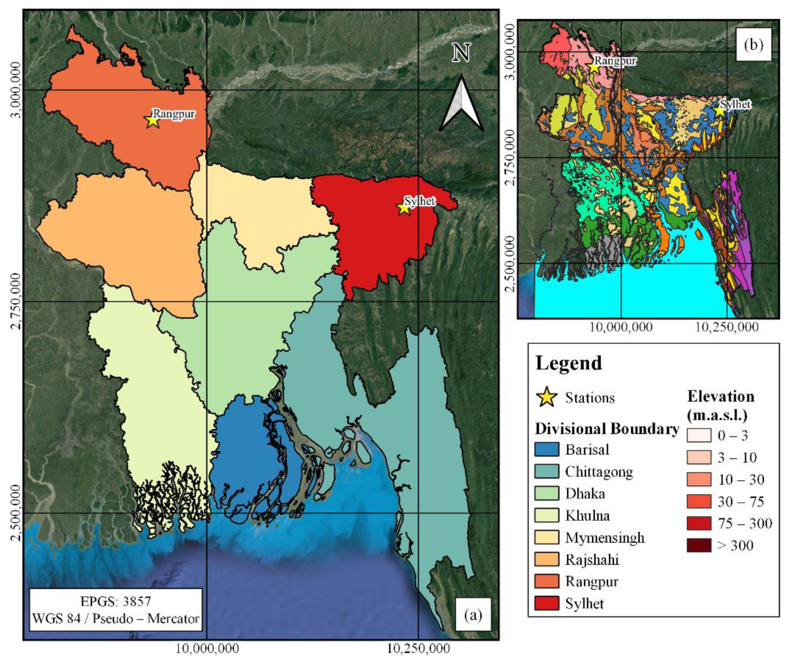
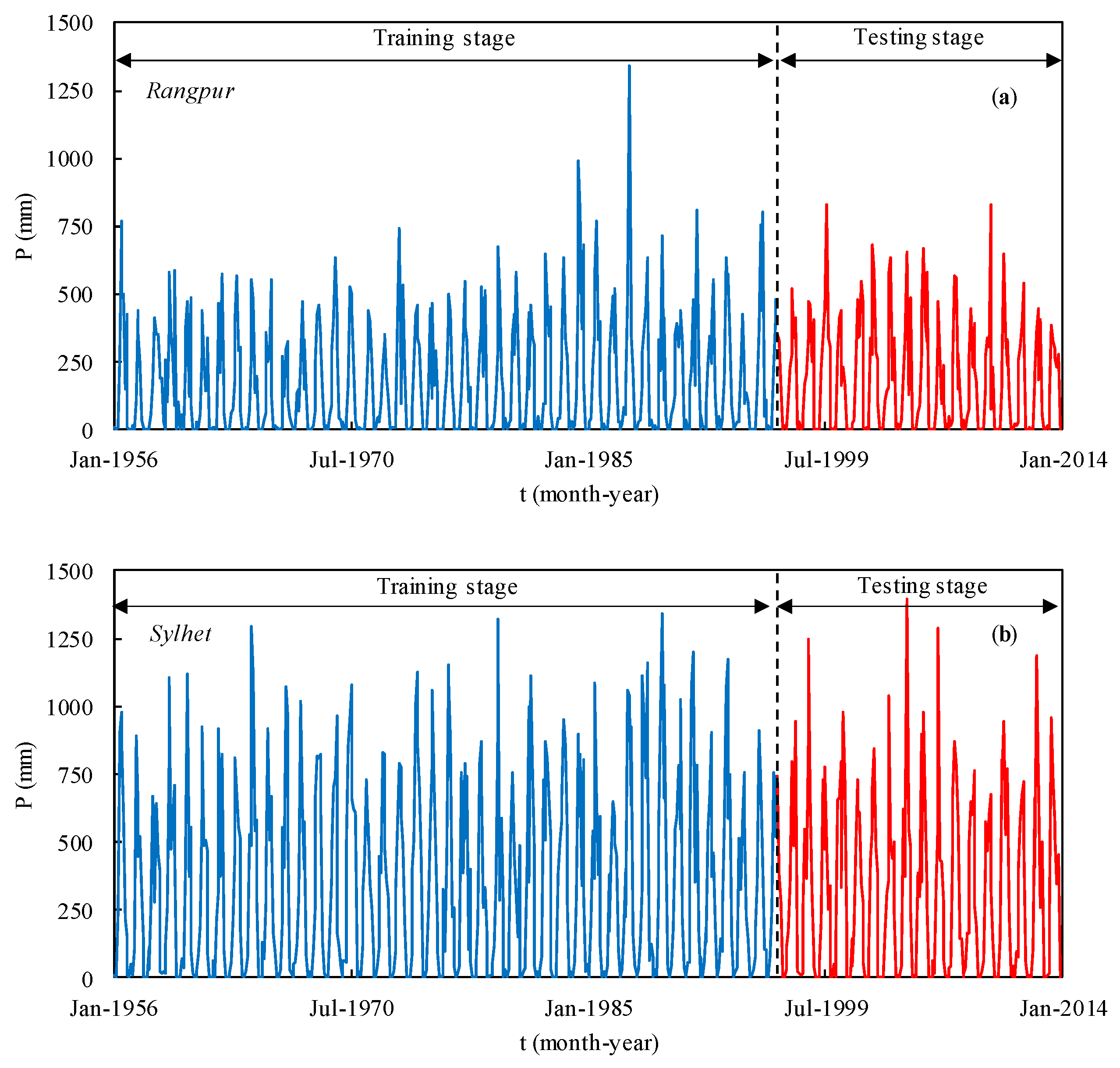
2. Study Area and Datasets

The study area consists of two divisions located in the northern region of Bangladesh: Rangpur and Sylhet. Rangpur Division shares its border with the Indian states of West Bengal, to the west and north, Assam and Meghalaya, to the east, and with the Bangladesh Division of Rajshahi to the south.

Sylhet Division shares its border with the Indian states of Meghalaya, to the north, Assam, to the east, and Tripura, to the south, and with the Bangladesh Division of Mymensingh and Dhaka, to the west, and Chittagong, to the southwest (Figure 1a). Elevations in the Rangpur Division range from values lower than 10 m in its southern area to 100 m in its northern area while in the Sylhet Division the terrain is flat, with an elevation that never exceeds 10 m (Figure 1b).

The physiographic of the Rangpur Division is mainly characterized by the floodplains, with alluvial fan deposits of both young and old gravelly sand, and the Barind clay deposits, that cover the southern part extending within the Rajshahi division. Sylhet Division is also covered by floodplains with alluvial silt and clay deposits, in particular in its central region, while in the western region, at the border with the Mymensingh and Dhaka Divisions and also in some areas of the central region, is covered by paludal deposits consisting in marsh clay and pea.

Overall, the climate in Northern Bangladesh is tropical monsoon with three distinct seasons: winter (between November and February), which is relatively cool with nearly no rainfall, pre-monsoon (between March and May), which is warm and characterized by thunderstorms, and monsoon (between June and October), with heavy rainfall [24]. Furthermore, due to its location just south of the Himalayas foothills, where monsoon winds blow from west and northwest, northeastern Bangladesh, in particular the Sylhet Division, receives the greatest average annual precipitation, over 4000 mm, while the national average is about 2550 mm [25].

Dataset consisted of time series measured from two monitoring stations, one in each division, both equipped with rain gauges for the precipitation measurement. The Rangpur station is located on a floodplain characterized by gravelly sands deposits, while the Sylhet station is situated on the paludal deposits of the central Sylhet. Monthly values of maximum temperature (T_max), minimum temperature (T_min), relative humidity (H), wind speed (V_wind), cloud coverage (C) and a monthly average of daily bright sunshine (S), were used for the precipitation (P) forecasting, from January 1956 to December 2013. Cloud coverage was measured in okta, ranging from 0 oktas, which indicates a completely clear sky, to 8 oktas, completely covered sky.

A normalization of the data with respect to the maximum values of each variable was performed, in order to improve forecasting efficiency [26], providing a common interval between 0 and 1. Moreover, datasets were split with a 70–30% ratio for training and testing stages, respectively [27,28,29].

Time series of precipitation for both Rangpur and Sylhet were reported in Figure 2.

Five different models were developed, allowing to evaluate the accuracy of the prediction as the number of exogenous inputs changes (

Table 1. Models developed based on the different exogenous inputs.

Model	Exogenous Inputs
A	Tmax, Tmin, H, Vwind, C, S
B	H, Vwind, C, S
C	Tmax, Tmin, H, Vwind
D	H, Vwind
E	H

). Furthermore, four evaluation metrics were computed to assess the accuracy of the ML algorithms [30,31]. The coefficient of determination (R²), which assess how well the model replicates measured values and predicts future values, the mean absolute error (MAE), equal to the average magnitude of the difference between measured and predicted values, the root mean square error (RMSE), equal to the root of the average square difference between measured and predicted values, and the relative absolute error (RAE), equal to the ratio between absolute error and absolute value of the difference between average of the measured value and each measured value. These metrics are defined as:

$${\mathrm{R}}^2=1-\frac{{{\displaystyle \sum }}_{i=1}^n{\left(P_{predicted,i}-P_{measured,i}\right)}^2}{{{\displaystyle \sum }}_{i=1}^n{\left(\overline{P}-P_{measured,i}\right)}^2}$$

(1)

$$\mathrm{MAE}=\frac{{{\displaystyle \sum }}_{i=1}^n\left|P_{predicted,i}-P_{measured,i}\right|}{n}$$

(2)

$$\mathrm{RMSE}=\sqrt{\frac{{{\displaystyle \sum }}_{i=1}^n{\left(P_{predicted,i}-P_{measured,i}\right)}^2}{n}}$$

(3)

$$\mathrm{RAE}=\frac{{{\displaystyle \sum }}_{i=1}^n\left|P_{predicted,i}-P_{measured,i}\right|}{{{\displaystyle \sum }}_{i=1}^n\left|\overline{P}-P_{measured,i}\right|}$$

(4)

where $P_{predicted,i}$ is the predicted precipitation for the i-th data, $P_{measured,i}$ is the measured precipitation for the i-th data; n is the total number of measured data; $\overline{P}$ is the mean value of the measured precipitation.

3. Methods

3.1. M5P

The M5P algorithm develops a regression tree, which is a decision tree with the real numbers as target variables, to get predictions [32]. Three different types of nodes are included in a regression tree: the root node, which includes the complete dataset, the internal nodes, which assign conditions on the input variables, and the leaf nodes, consisting of linear regression models of the target values.

The input dataset is iteratively divided into sub-domains, in which multivariable linear regression models are built, in the development process. In particular, the first step consists of a subdivision of the dataset into two subsets, assessing the possible binary split. In the subsequent steps, each subset is divided into smaller subsets considering the couple of subsets that maximized a least-squared deviation (LSD) function, with:

$$R\left(t\right)=\frac{1}{N\left(t\right)}{\displaystyle \sum }_{i\in t}\left(y_i-y_m\left(t\right)\right)$$

(5)

where R(t) is the within variance in the node t, N indicates the number of subset units, y_i is the target variable value for the i-th unit, and y_m is the target variable mean. The function Φ(s_p, t) to be maximized is expressed as:

$$\Phi \left(s_p,t\right)=R\left(t\right)-p_{L}R\left(t_L\right)-p_{R}R\left(t_R\right)$$

(6)

where p_L and p_R are the portion units allocated to the left node t_L and right node t_R, and s_p indicated the split value [33]. Different stopping rules were considered: minimum impurity level, minimum impurity change in the subdivision, minimum elements number for each node, and maximum tree depth. Furthermore, the pruning technique was considered to avoid overfitting problems for the fully developed tree. This technique removes branches that provide a low contribution to the prediction ability in order to reduce the tree size. The following parameters were considered: Batch size = 100; minimum number of instances to allow at a leaf node = 6.

3.2. Support Vector Regression (SVR)

Support vector machine algorithms (SVMs) are supervised learning models with associated learning algorithms. SVMs have proved to be among the most robust prediction algorithms, being particularly efficient for classification and regressions analysis [34,35,36]. These are assumed and proven to be highly robust in nature for extremely noise-mixed data in comparison to the other local models and algorithms which use traditional chaotic methods. Furthermore, SVMs are more reliable for noise-mixed data in comparison to other models and algorithms based on traditional chaotic methods. When applied to regression problems, the SVM algorithm is generally called support vector regression (SVR).

The objective of the SVR is to find a function f(x) with a deviation lower than a value ε from the target values y_i. Based on the following training dataset: {(x_i, y_i), i = 1, …, l} ⊂ X × R, where X indicates the space of the input arrays, the Euclidean norm ||w||² must be minimized, by solving a constrained convex optimization problem, in order to find a linear function f(x) = 〈w, x〉 + b, where b ∈ R and w ∈ X. In addition, slack variables were introduced to tolerate to allow deviations from ε.

The optimization can be expressed as:

$$\mathrm{minimize}:\frac{1}{2}{\Vert w\Vert }^2+C{{\displaystyle \sum }}_{i=1}^l\left({\xi }_i+{\xi }_i^{*}\right)$$

(7)

$$\mathrm{subject}\mathrm{to}:\begin{array}{c}{y}_i-\langle w,x_i\rangle -b\le \epsilon +{\xi }_i\\ \langle w,x_i\rangle +b-y_i\le \epsilon +{\xi }_i^{*}\end{array}$$

(8)

where deviation and function flatness depend on the constant C, which is greater than 0 [37]. The effectiveness of SVR depends also on the selection of the kernel function, which defines the feature space, and of its parameters. The Pearson VII universal function kernel (PUK) was considered, whose parameters were optimized through the PSO algorithm. PUK kernel can be expressed as:

$$k\left(x_i,x_j\right)=\frac{1}{{\left[1+{\left(\left(2\sqrt{{\left|x_i-x_j\right|}^2\sqrt{2^{\left(1/\omega \right)}-1}}\right)/\sigma \right)}^2\right]}^{\omega }}$$

(9)

with σ and ω that control the half-width and the tailing factor of the peak, respectively.

3.3. Hybrid Model M5P-SVR

In order to improve the modeling performances, based on the predictions made with the M5P and SVR algorithms, it is possible to build hybrid models, leading to better forecasts. A key parameter to configure the hybrid model is how the predictions performed by the single algorithms are combined. More details on the rules for the combination of classifiers are reported in Kittler et al. (1998) [38]. In the present study, the average of probabilities was considered as the combination rule, which evaluates the mean value of each class among the independent classifiers [39].

The parameters considered for the individual algorithms, M5P and SVR, within the hybrid model, were the same reported in the previous sections.

3.4. Particle Swarm Optimization (PSO)

The particle swarm optimization (PSO) is a well-known algorithm, which is widely applied in optimization problems, including the parameters calibration of machine learning algorithms in order to improve their performance in hydrological applications [40,41,42]. PSO is a population-based technique that was motivated by studying the social behavior of fish and birds in finding the shortest route to find the food [43]. The PSO performs an iterated research based on a population, namely as a swarm, of individuals, namely as particles. The velocity update equation manages the population as it moves through the search space searching of the optimal state. In each iteration, the algorithm saves the local optimum value and compares it with the global ones, with the optimum state which is chosen based on the fitness of an objective function [44]. In addition, due to its high learning speed and the low memory requirement, the PSO algorithm was used to solve several non-linear applications in hydrologic field [45,46]. The PSO algorithm was applied to optimize the following parameters for SVR: Batch size = 100; C = 1.0; Kernel = PUK with σ = 2.0 and ω = 0.1.

4. Results

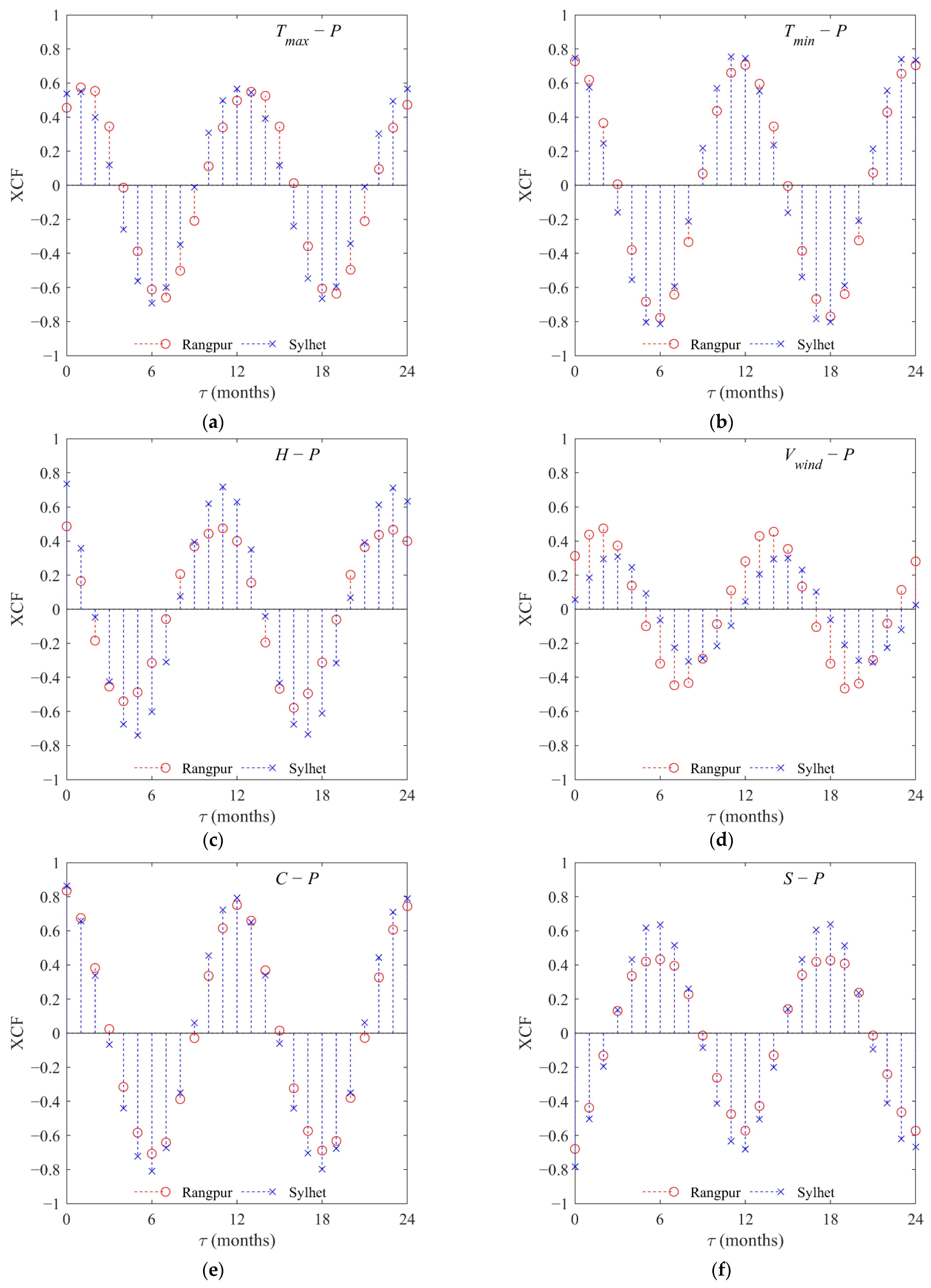
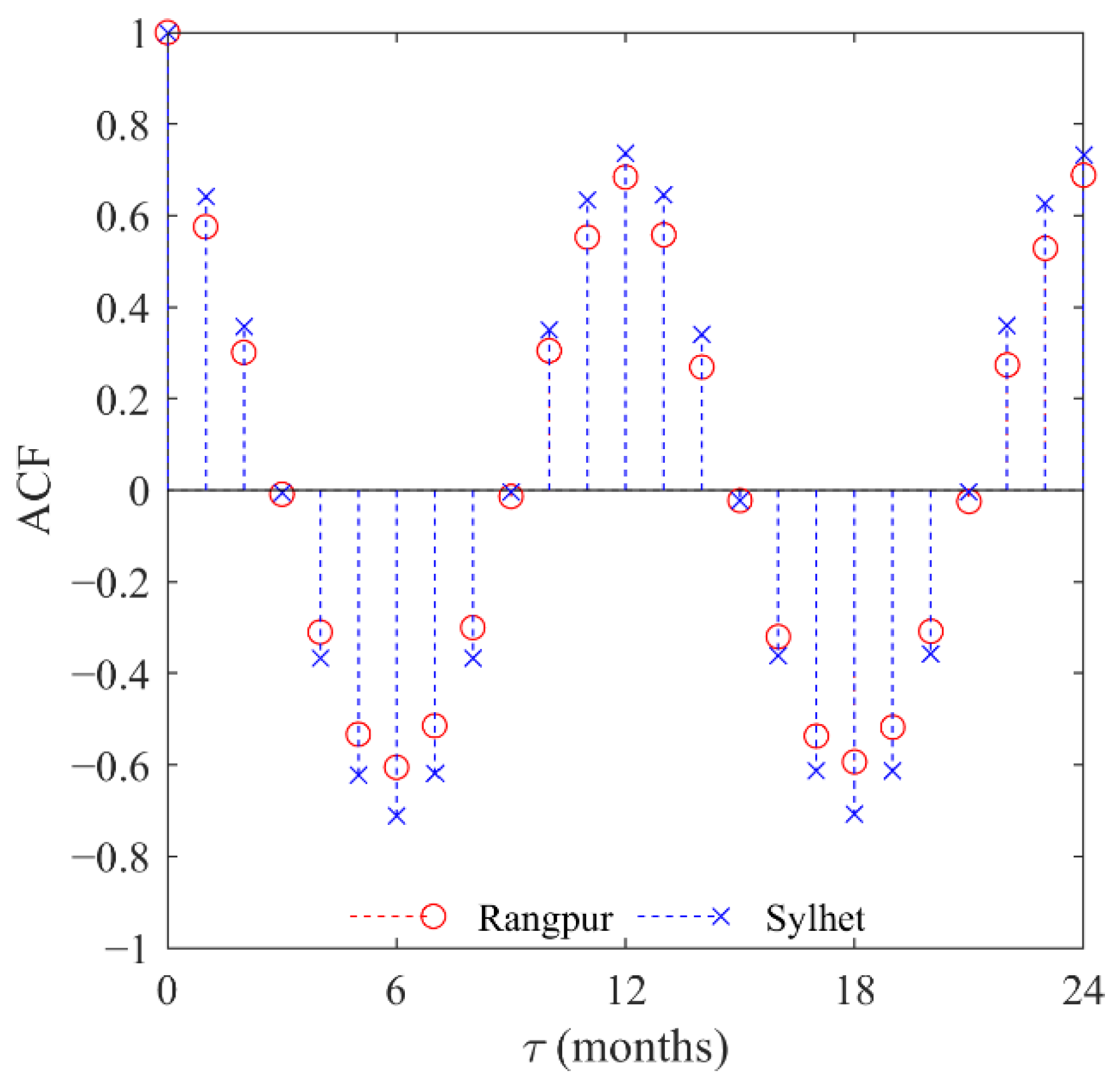
4.1. Time Series Analysis

Figure 3 shows a bar plot of the average monthly precipitation for Rangpur and Sylhet from 1956 to 2013. Maximum precipitations were observed during the monsoon season, equal to 457 mm for Rangpur and 799 mm for Sylhet, in July and June, respectively. Minimum precipitations were instead observed for the dry season, equal to 8 mm for both Rangpur and Sylhet, in January and December, respectively.

During the dry season, from November to February, both stations showed values of the average monthly precipitation lower than 30 mm. However, pre-monsoon season highlighted marked difference between the two stations, with average monthly precipitation that increased from 29 mm in March to 263 mm in May for Rangpur and from 114 mm in March to 571 mm in May for Sylhet.

These differences became even more marked during the monsoon season until they fade at the end of the season, in the month of October, where the two stations showed similar average precipitations (170 mm for Rangpur and 218 mm for Sylhet). Overall, the mean annual rainfall estimated in the monitored period was equal to 2149 mm for Rangpur and 4004 mm for Sylhet.

Table 2. Statistics for Rangpur and Sylhet stations.

Variable	Rangpur					Sylhet
	Mean	σ	CV	Max	Min	Mean	σ	CV	Max	Min
Tmax (°C)	32.9	3.6	0.11	43.3	21.6	33.2	2.8	0.08	39.6	25.8
Tmin (°C)	19.9	5.5	0.28	27.7	7.3	20.3	4.5	0.22	26.3	10.6
P (mm)	179.1	203.9	1.14	1344.0	0.0	333.7	336.3	1.01	1394.0	0.0
H (%)	80.6	7.1	0.09	92.0	40.0	78.7	8.1	0.10	93.0	47.0
Vwind (m/s)	1.2	0.6	0.50	3.3	0.2	1.5	0.7	0.47	5.4	0.3
C (okta)	3.3	2.0	0.61	7.2	0.1	4.3	2.2	0.51	7.7	0.3
S (hours)	6.4	1.5	0.23	10.8	1.7	6.3	2.0	0.32	10.6	0.0

provides the statistics of the monthly data for both Rangpur and Sylhet stations, where σ indicates the standard deviation and CV the coefficient of variation, equal to the ratio between σ and mean.

For the input selection, different techniques can be used, e.g., average mutual information [47] and Akaike Selection Criterion (AIC) [48]. In the present study, the cross-correlation function (XCF) and auto-correlation function (ACF) were used to assess the feedback delay between the exogenous input variables and the precipitation (Figure 4) and the input delay (Figure 5), respectively. This approach is in agreement with different machine-learning-based models developed to solve hydrological problems [49,50]. XCF is expressed as:

$$\mathrm{XCF}=\underset{0}{\overset{s}{{\displaystyle \int }}}I\left(t\right)·\left[P\left(t+\tau \right)\right]d\tau$$

(10)

where I is the exogenous input variable, s is the duration of the time series, and τ the delay [51]. Patterns between the two stations were very similar. In particular, T_min (Figure 4b) showed XCF peaks equal to 0.8, higher than those computed for T_max (Figure 4a), equal to 0.6, highlighting a greater correlation of the minimum temperatures with the precipitation. Both peaks were observed for τ = 12 months. The cross-correlation between relative humidity and precipitation (Figure 4c) exhibited peaks at τ = 11 months for both stations. A higher correlation for Sylhet was computed, with XCF close to 0.8. However, Rangpur also showed a good correlation, with XCF higher than 0.5. For the cross-correlation between wind speed and precipitation, peaks were instead observed for a τ = 14 months (Figure 4d), with a lower correlation in comparison to temperature and humidity, with XCF = 0.4 for Rangpur and XCF = 0.3 for Sylhet. Cross-correlation between cloud coverage and precipitation (Figure 4e) showed high peaks at τ = 12 months, with XCF close to 0.8 for both stations.

The cross-correlation between bright sunshine and precipitation (Figure 4f) showed an opposite trend in comparison with the other exogenous input, with XCF positive peak equal to 0.4 for Rangpur and 0.6 for Sylhet at τ = 6 months. However, for τ = 12 months a greater XCF negative peak, in absolute value, was computed, equal to −0.6 for Rangpur and −0.7 for Sylhet. The strong negative correlation is closely linked to the tropical monsoon climate of the region. During the monsoon season, heavy rainfalls are followed by a reduced number of hours of sunshine per day, up to a minimum monthly average value of 2 h a day in July and August, while, during the winter and pre-monsoon seasons, sunny days with low rainfalls prevail, with a maximum monthly average value of 9 h a day in December and January.

The auto-correlation function (ACF), which was also computed for both stations which is expressed as:

$$\mathrm{ACF}=\underset{0}{\overset{s}{{\displaystyle \int }}}P\left(t\right)·P\left(t+\tau \right)d\tau$$

(11)

Also in this case, similar patterns were found between the two stations, with a similar positive peak ACF close to 0.8 for a delay τ = 12 months. This strong autocorrelation can be related to the seasonal nature of the precipitation. ACF results were in agreement with Chowdhury et al. (2019) [52], which also investigate the monthly precipitations for different stations located in the Sreemangal sub-district of the Sylhet Division.

Overall, based on the XCF and ACF analyses, both delays for exogenous inputs and targets were set to 12 months.

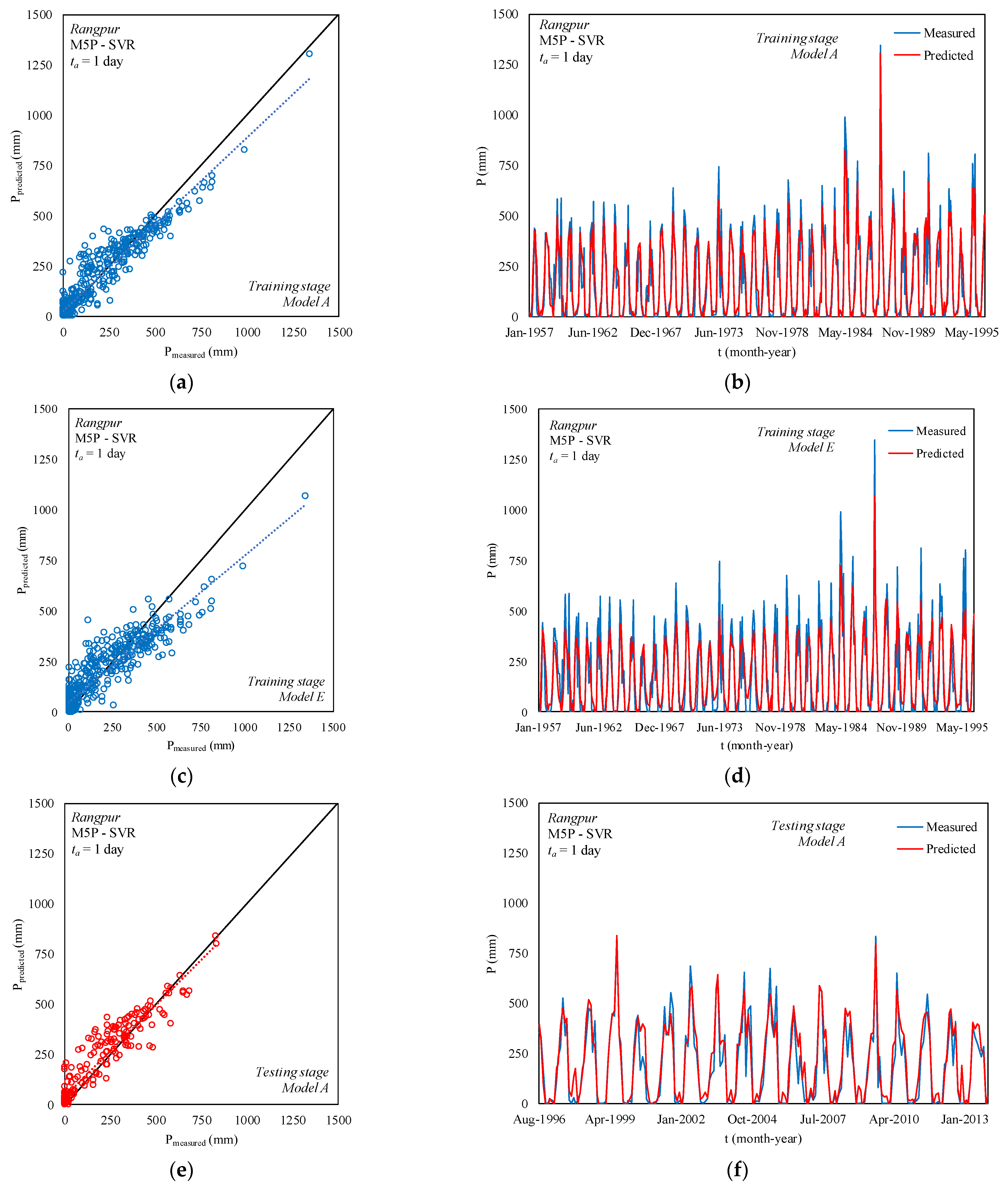
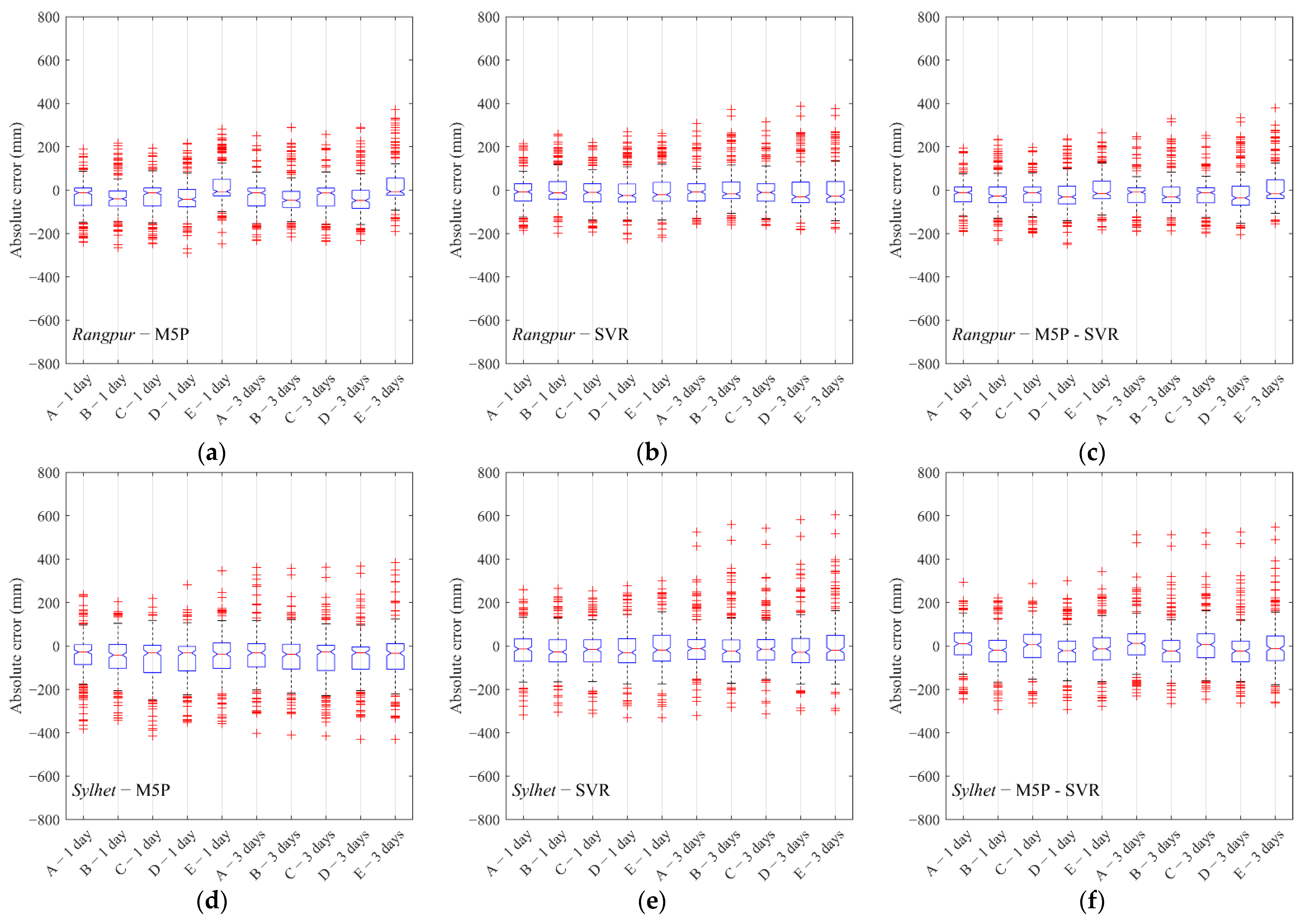
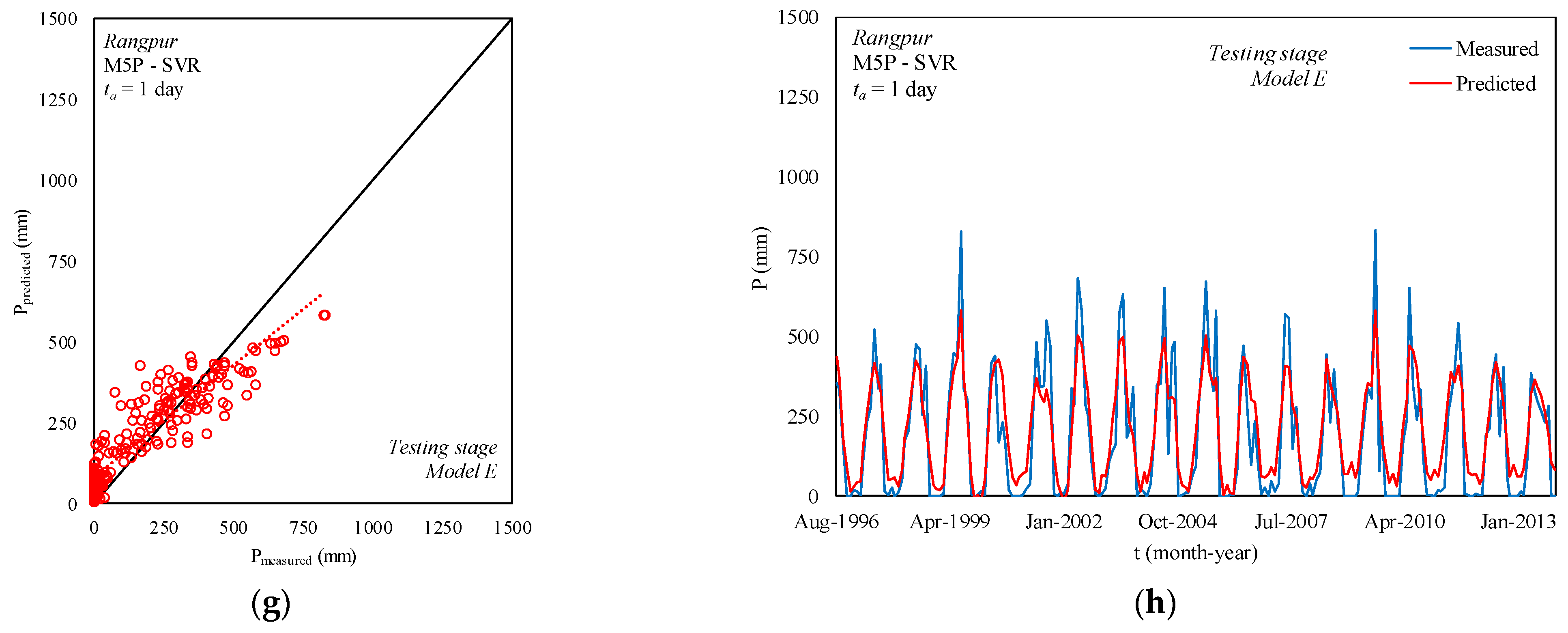
4.2. Rangpur Station

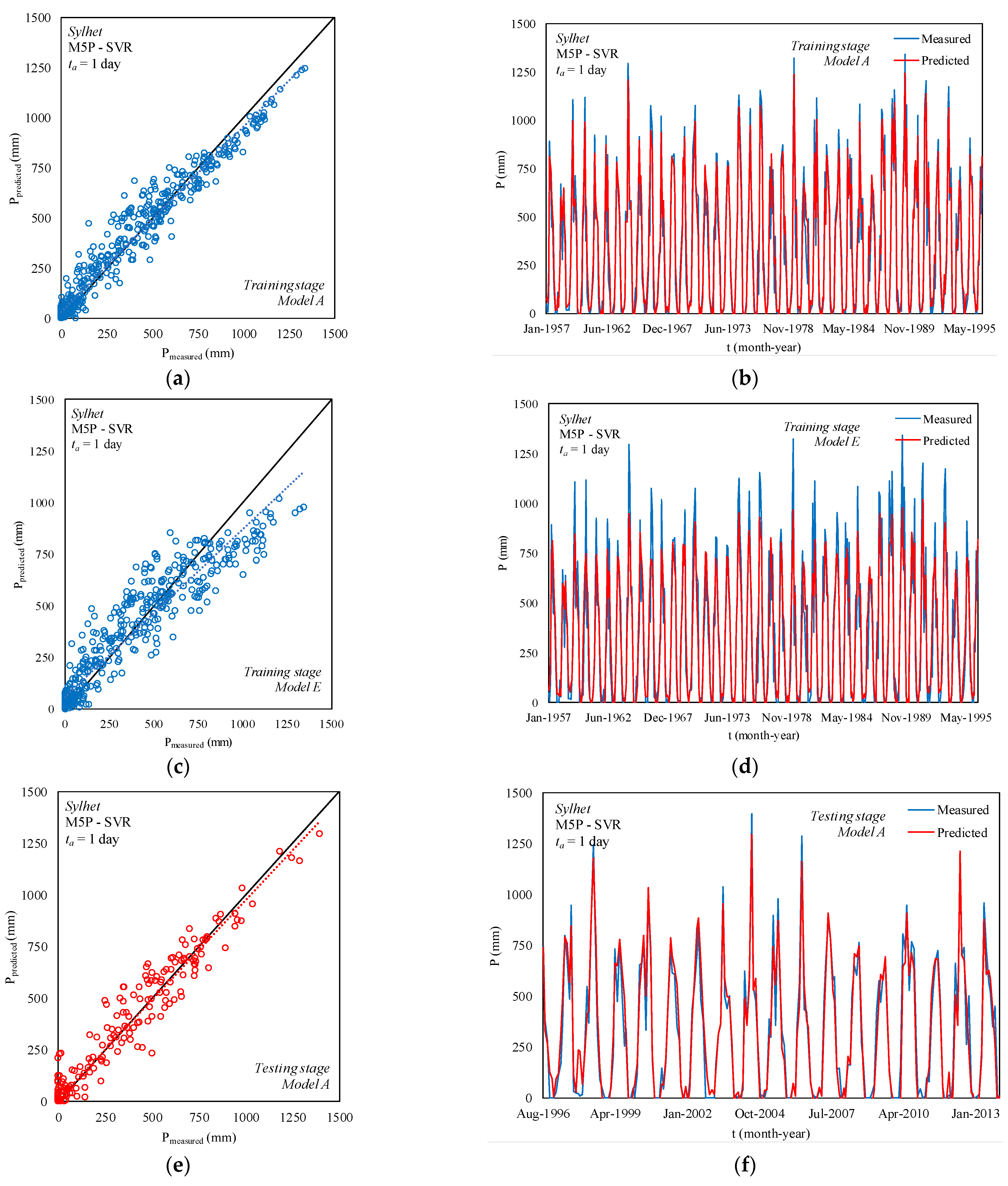
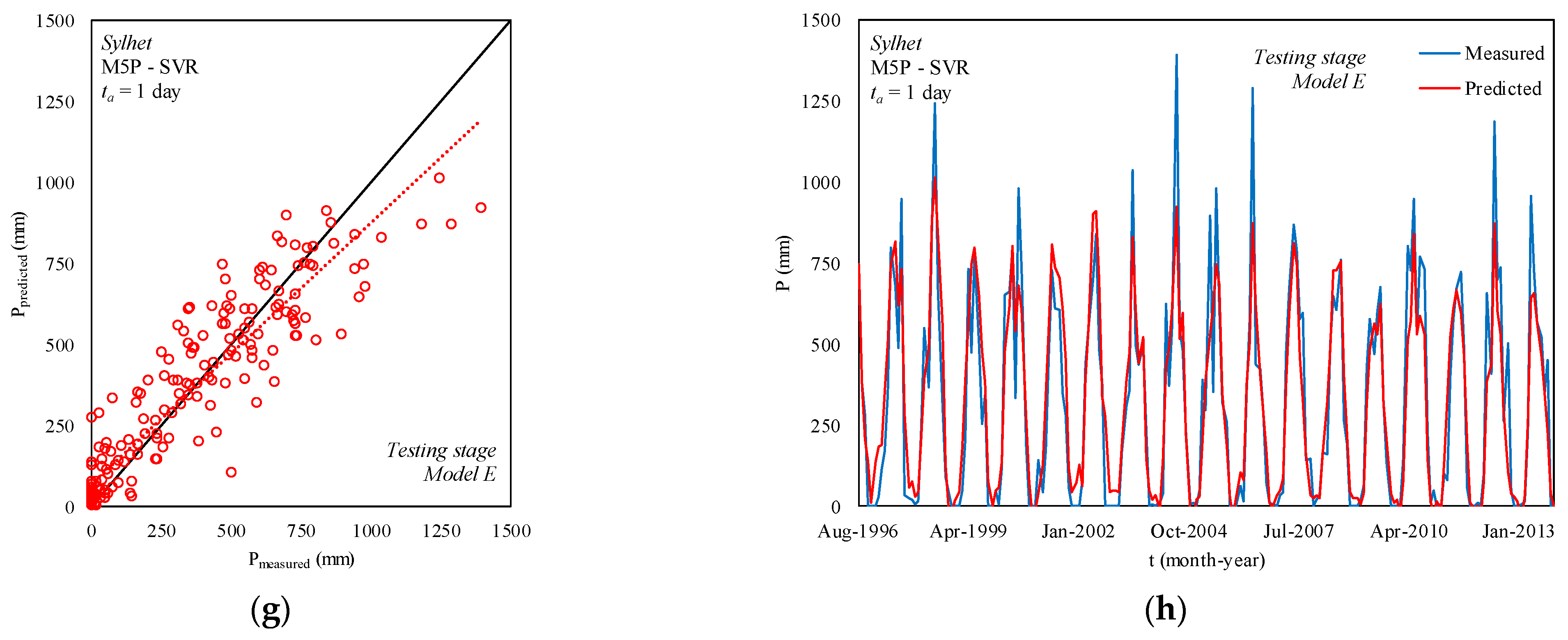
Predictions obtained for the Rangpur station are discussed in this section. The evaluation metrics computed for the training and testing stages are reported in

Table 3. Evaluation metrics computed for the Rangpur station.

Stage	ta	Algorithm	Metrics	Model
				A	B	C	D	E
Training	1 month	M5P	R2	0.88	0.85	0.87	0.80	0.79
			MAE (mm)	47	53	48	64	67
			RMSE (mm)	71	77	73	86	90
			RAE (%)	28.05	30.88	28.04	37.55	39.59
		SVR	R2	0.85	0.79	0.85	0.78	0.77
			MAE (mm)	51	61	52	62	65
			RMSE (mm)	75	88	78	89	92
			RAE (%)	30.13	35.55	30.09	37.05	38.12
		M5P-SVR	R2	0.89	0.87	0.87	0.80	0.79
			MAE (mm)	47	49	47	62	64
			RMSE (mm)	68	71	71	85	88
			RAE (%)	27.42	28.31	27.52	36.44	37.98
	3 months	M5P	R2	0.88	0.84	0.87	0.79	0.78
			MAE (mm)	48	54	49	65	69
			RMSE (mm)	71	78	73	86	89
			RAE (%)	28.22	31.48	28.24	38.25	40.69
		SVR	R2	0.85	0.77	0.84	0.76	0.74
			MAE (mm)	52	62	52	65	67
			RMSE (mm)	76	91	78	94	95
			RAE (%)	30.33	36.46	30.35	38.42	39.52
		M5P-SVR	R2	0.89	0.87	0.87	0.79	0.78
			MAE (mm)	47	49	47	63	66
			RMSE (mm)	69	71	71	87	90
			RAE (%)	27.50	28.73	27.50	37.20	39.25
Testing	1 month	M5P	R2	0.86	0.82	0.86	0.80	0.72
			MAE (mm)	69	75	69	83	84
			RMSE (mm)	96	91	96	95	103
			RAE (%)	41.99	44.84	42.02	48.64	49.41
		SVR	R2	0.84	0.79	0.83	0.78	0.78
			MAE (mm)	66	74	67	79	79
			RMSE (mm)	91	94	92	97	98
			RAE (%)	40.51	43.73	41.05	46.46	46.89
		M5P-SVR	R2	0.87	0.82	0.86	0.80	0.79
			MAE (mm)	62	73	65	76	79
			RMSE (mm)	88	91	89	92	94
			RAE (%)	38.09	43.15	39.65	45.04	46.56
	3 months	M5P	R2	0.86	0.82	0.86	0.79	0.72
			MAE (mm)	69	75	69	86	87
			RMSE (mm)	97	93	97	98	104
			RAE (%)	42.35	50.81	42.39	44.35	51.70
		SVR	R2	0.83	0.79	0.83	0.77	0.77
			MAE (mm)	67	75	68	82	83
			RMSE (mm)	92	95	92	99	100
			RAE (%)	40.81	44.83	41.40	48.38	49.05
		M5P-SVR	R2	0.87	0.82	0.86	0.80	0.78
			MAE (mm)	63	75	65	78	83
			RMSE (mm)	89	93	90	93	96
			RAE (%)	38.45	44.25	39.71	46.16	48.94

.

For the training stage, with a lag time t_a = 1 month, the best performances were obtained with the hybrid algorithm M5P-SVR and Model A, which included all the monitored exogenous inputs (R² = 0.89, MAE = 47 mm, RMSE = 68 mm, MAE = 27.42%, Figure 6a,b). Performances reduced passing to Model B, which did not consider T_max and T_min as exogenous inputs (R² = 0.87, MAE = 49 mm, RMSE = 71 mm, MAE = 28.31%). Model B was outperformed by Model C, which instead did not include the cloud overage and the daily bright sunshine as exogenous inputs, while it took into account both maximum and minimum temperatures (R² = 0.87, MAE = 47 mm, RMSE = 71 mm, MAE = 27.52%). This highlights a greater impact on the algorithms training of the temperature, in comparison with the cloud coverage and bright sunshine. However, Model D (R² = 0.80, MAE = 62 mm, RMSE = 85 mm, MAE = 36.44%), which included only H and V_wind as exogenous inputs, exhibited much lower performances with respect to both Models B and C. Therefore, not considering the cloud overage and the daily bright sunshine as exogenous inputs still had a negative impact on the algorithms training. The worst performances were achieved for Model E (R² = 0.79, MAE = 64 mm, RMSE = 88 mm, MAE = 37.98%, Figure 6c,d), which included only the relative humidity as exogenous input. Both M5P and SVR algorithms showed similar performances reduction passing from Model A (M5P–R² = 0.88, MAE = 47 mm, RMSE = 10,471 mm, MAE = 28.05%; SVR–R² = 0.85, MAE = 51 mm, RMSE = 75 mm, MAE = 30.13%) to Model E (M5P–R² = 0.79, MAE = 67 mm, RMSE = 90 mm, MAE = 39.59%; SVR–R² = 0.77, MAE = 65 mm, RMSE = 92 mm, MAE = 38.12%). However, a marked difference between the algorithms was observed for Model B, with M5P (R² = 0.85, MAE = 53 mm, RMSE = 77 mm, MAE = 30.88%) that showed better performances in comparison with SVR (R² = 0.79, MAE = 61 mm, RMSE = 88 mm, MAE = 35.55%). As the lag time increases, from t_a = 1 month to t_a = 3 months, a slight performance reduction was observed for all algorithms and models. However, M5P-SVR with Model A was confirmed as the most performing algorithm (R² = 0.89, MAE = 47 mm, RMSE = 69 mm, MAE = 27.50%).

For the testing stage, the best predictions were achieved also with the hybrid algorithm M5P-SVR and Model A, with no relevant difference as the lag time increases (t_a = 1 month–R² = 0.87, MAE = 62 mm, RMSE = 88 mm, MAE = 38.09%, Figure 6e,f; t_a = 3 months–R² = 0.87, MAE = 63 mm, RMSE = 89 mm, MAE = 38.45%). It should be noted that, passing from the training to the testing stage, only a slight performance reduction was observed. The difference in terms of performances between Model B and Model C, observed for the training stage in particular for SVR, has been observed also for the hybrid model M5P-SVR for the testing stage (t_a = 1 month, Model B–R² = 0.82, MAE = 73 mm, RMSE = 91 mm, MAE = 43.15%; t_a = 1 month, Model C–R² = 0.86, MAE = 65 mm, RMSE = 89 mm, MAE = 39.65%). However, the worst predictions were achieved with Model E, for both lag times (t_a = 1 month, R² = 0.79, MAE = 79 mm, RMSE = 94 mm, MAE = 46.56%, Figure 6g,h; t_a = 3 months, R² = 0.78, MAE = 83 mm, RMSE = 96 mm, MAE = 48.94%).

Overall, SVR algorithm led to predictions in line, in terms of accuracy, with M5P algorithm. However, while for Model A the M5P (t_a = 1 month, R² = 0.86, MAE = 69 mm, RMSE = 96 mm, MAE = 41.99%) led to slightly better prediction in comparison with SVR (t_a = 1 month, R² = 0.84, MAE = 66 mm, RMSE = 91 mm, MAE = 40.51%), for Model E, SVR (t_a = 1 month, R² = 0.78, MAE = 79 mm, RMSE = 98 mm, MAE = 46.89%) outperformed significantly M5P (t_a = 1 month, R² = 0.72, MAE = 84 mm, RMSE = 103 mm, MAE = 49.41%) for both lag times.

4.3. Sylhet Station

This section shows the precipitation forecasts for the Sylhet station, with the performances for both training and testing stages reported in

Table 4. Evaluation metrics computed for the Sylhet station.

Stage	ta	Algorithm	Metrics	Model
				A	B	C	D	E
Training	1 month	M5P	R2	0.92	0.90	0.91	0.89	0.88
			MAE (mm)	62	68	66	73	84
			RMSE (mm)	85	95	92	102	114
			RAE (%)	21.14	24.21	22.98	25.32	28.87
		SVR	R2	0.90	0.86	0.88	0.84	0.84
			MAE (mm)	62	75	68	81	88
			RMSE (mm)	89	106	98	116	124
			RAE (%)	21.45	25.95	23.54	28.42	30.30
		M5P-SVR	R2	0.94	0.93	0.93	0.91	0.88
			MAE (mm)	55	59	58	64	82
			RMSE (mm)	76	84	83	91	112
			RAE (%)	18.64	20.67	20.28	22.38	28.28
	3 months	M5P	R2	0.92	0.90	0.91	0.89	0.88
			MAE (mm)	63	70	67	75	86
			RMSE (mm)	85	97	93	104	118
			RAE (%)	21.50	24.38	23.30	26.48	34.30
		SVR	R2	0.89	0.85	0.88	0.84	0.84
			MAE (mm)	64	75	69	82	90
			RMSE (mm)	90	108	99	117	126
			RAE (%)	21.89	26.24	24.08	28.77	30.64
		M5P-SVR	R2	0.94	0.92	0.92	0.90	0.88
			MAE (mm)	56	62	60	69	85
			RMSE (mm)	78	85	85	95	114
			RAE (%)	19.12	21.37	20.83	24.35	28.99
Testing	1 month	M5P	R2	0.91	0.87	0.87	0.87	0.85
			MAE (mm)	77	83	83	89	102
			RMSE (mm)	99	113	111	121	133
			RAE (%)	28.60	31.13	31.16	33.27	35.96
		SVR	R2	0.91	0.84	0.86	0.82	0.82
			MAE (mm)	69	78	73	83	92
			RMSE (mm)	92	106	99	118	125
			RAE (%)	25.38	27.58	27.39	31.74	34.08
		M5P-SVR	R2	0.92	0.89	0.89	0.88	0.85
			MAE (mm)	68	73	73	77	86
			RMSE (mm)	91	99	99	107	119
			RAE (%)	25.26	27.45	27.12	29.34	31.84
	3 months	M5P	R2	0.90	0.87	0.87	0.85	0.83
			MAE (mm)	80	86	87	92	106
			RMSE (mm)	103	117	117	130	147
			RAE (%)	29.31	32.26	32.63	34.79	37.70
		SVR	R2	0.90	0.84	0.87	0.83	0.82
			MAE (mm)	70	80	75	86	93
			RMSE (mm)	93	108	102	116	126
			RAE (%)	25.86	28.03	27.95	32.03	34.37
		M5P-SVR	R2	0.91	0.87	0.88	0.86	0.83
			MAE (mm)	69	75	74	79	89
			RMSE (mm)	93	102	100	109	122
			RAE (%)	25.57	27.94	27.73	30.07	32.87

.

For the training stage, the best performances were observed for the hybrid model M5P-SVR with Model A, for both lag times (t_a = 1 month–R² = 0.94, MAE = 55 mm, RMSE = 76 mm, MAE = 18.64%, Figure 7a,b; t_a = 3 months–R² = 0.94, MAE = 56 mm, RMSE = 78 mm, MAE = 19.12%). As the number of exogenous inputs reduces, a performance decrease was observed. In particular, Models B and C exhibited performances similar to each other and lower to Model A, for both lag times. A further slight performance decrease occurs passing to Model D (t_a = 1 month–R² = 0.91, MAE = 64 mm, RMSE = 91 mm, MAE = 22.38%; t_a = 3 months–R² = 0.90, MAE = 69 mm, RMSE = 95 mm, MAE = 24.35%). However, a marked performance decrease occurs passing from Model D to Model E, with the latter that considered only the relative humidity as exogenous input (t_a = 1 month–R² = 0.88, MAE = 82 mm, RMSE = 112 mm, MAE = 28.28%, Figure 7c,d; t_a = 3 months–R² = 0. 88, MAE = 85 mm, RMSE = 114 mm, MAE = 28.99%).

Both M5P and SVR algorithms led to lower performances in comparison with the hybrid model. However, M5P outperformed SVR for both lag times and for all the five models, with higher R² values and lower values of MAE, RMSE, and MAE.

For the testing stage, hybrid model M5P-SVR was confirmed as the best algorithm, for all models and lag times. In particular, Model A led to the best predictions with a slight performance decrease passing from t_a = 1 month (R² = 0.92, MAE = 68 mm, RMSE = 91 mm, MAE = 25.26%, Figure 7e,f) to t_a = 3 months (R² = 0.91, MAE = 69 mm, RMSE = 93 mm, MAE = 25.57%). As for the training stage, performances of Model B and Model C were in line and lower than those computed for Model A. Model D (t_a = 1 month–R² = 0.88, MAE = 77 mm, RMSE = 107 mm, MAE = 29.34%; t_a = 3 months–R² = 0.86, MAE = 79 mm, RMSE = 109 mm, MAE = 30.07%) was slightly outperformed by both models B and C, proving its reliability despite it included only relative humidity and the wind speed as exogenous inputs. A lower prediction ability was observed for Model E (t_a = 1 month, R² = 0.85, MAE = 86 mm, RMSE = 119 mm, MAE = 31.84%, Figure 7g,h; t_a = 3 months, R² = 0.83, MAE = 89 mm, RMSE = 122 mm, MAE = 32.87%). However, the hybrid model M5P-SVR with Model E, even including the only relative humidity as exogenous input, was still able to properly detect the precipitations trend.

As for the Rangpur station, SVR led to predictions in line with M5P algorithm. However, both individual M5P and SVR were outperformed by the hybrid model M5P-SVR. It should be noted that also the individual M5P and SVR algorithms did not show particularly marked reductions in performances as the number of exogenous inputs decreased, with Model E that exhibited quite good performances for both algorithms and lag times (M5P-t_a = 1 month, R² = 0.85, MAE = 102 mm, RMSE = 133 mm, MAE = 35.96%; SVR-t_a = 1 month, R² = 0.82, MAE = 92 mm, RMSE = 125 mm, MAE = 34.08%).

4.4. Performance Comparisons of the Models

Figure 8 shows the box plots of absolute errors, providing further analysis of the precipitation predictions performed with the different algorithms and models for the two stations of Rangpur and Sylhet. Absolute errors are expressed as the differences between measured and predicted precipitations. Therefore, a positive error denotes an underestimation of the measured value while a negative error denotes an overestimation of the same.

For Rangpur station, M5P box plot (Figure 8a) showed notches, which reflect the 95% confidence interval of the median, between −84 mm for Model D-t_a = 3 days and 55 mm for Model E-t_a = 3 days, while outliers (indicated with the red crosses) with positive and negative absolute errors between −291 mm and 370 mm. Overall, Model E led to the higher underestimation of heavy rainfalls. A narrow box plot was computed for Model A with a notch between −70 mm and 9 mm, a median equal to −14 mm and the outliers between −240 mm and 190 mm. SVR box plot (Figure 8b) showed similar results, with the exception of the Model E for which the SVR algorithm led to a narrower box plot in comparison with the M5P one. The narrowest box plots and the lowest outliers where, however, computed for the hybrid model M5P-SVR (Figure 8c) with a notch for Model A between −54 mm and 14 mm and a median equal to −11 mm.

For Sylhet station, M5P box plot (Figure 8d) exhibited more asymmetrical notches in comparison with Rangpur with a notch for Model A between −85 mm and 6 mm and a median equal to −18 mm.

SVR (Figure 8e) and M5P-SVR (Figure 8f) notches were instead more symmetrical, following an almost normal distribution of absolute errors. In Particular, for M5P-SVR and Model A, the notch was between −40 mm and 60 mm with the median equal to 10 mm. It should be noted that higher positive outliers where instead computed for both SVR and M5P-SVR, up to values close to 600 mm, while M5P led to outliers lower than 400 mm. On the other hand, the negative outliers reached values close to −320 mm and −300 mm for SVR and M5P-SVR, respectively, which were lower (in absolute value) than those reached with the M5P algorithm, close to −430 mm.

5. Discussion

The performance of the machine learning algorithms was assessed for the precipitation modeling for two stations located in Northern Bangladesh. Results revealed that ML algorithms, with particular reference to the hybrid model M5P-SVR, should be reliable for the precipitation prediction in tropical monsoon-climate areas.

In particular, for M5P-SVR, the scatter plots between measured and predicted precipitation for the two stations (Figure 6 and Figure 7 on the left) exhibited regression lines (dotted lines) located just above the best fit line (continuous lines) for the Model A, which considered all the available exogenous inputs. Major discrepancies between the two lines were observed for Model E, which includes the only relative humidity as input.

Further comparison between individual algorithms and the hybrid one was made using box plots (Figure 8). The result confirmed that M5P-SVR combined with Model A led to the narrower notches and to the lower absolute errors in comparison with the individual algorithms and the other models, for both stations and lag times.

A further interesting aspect is represented by the ability of the developed models to provide accurate predictions of extreme events. The difficulties in providing an accurate estimate of extreme precipitation events also appear clear from recent literature studies [20,22]. However, as shown in the time series with the measured and predicted precipitation for the two stations (Figure 6e,f and Figure 7e,f) M5P-SVR model combined with Model A led to good prediction also of relevant peaks, with precipitation higher than 750 mm and 1000 mm, respectively for Rangpur and Sylhet. It should be noted that as the number of exogenous inputs reduces, there is a marked reduction in the accuracy of the peaks prediction, this is particularly visible for Model E (Figure 6g,h and Figure 7g,h).

Predictions obtained from this study were also compared with recent work conducted in areas with different climates. Chiang et al. (2007) [5] for the subtropical climate of Taiwan, where typhoons, usually coupled with heavy rainfall, hit the island more than three times a year, modeling short-term daily rainfall time series with a recurrent neural network (RNN), leading to R² values up to 0.63. Pham et al. (2020) [20] model the short-term daily rainfall for the tropical climate of Vietnam, reaching R² values up to 0.69 with the SVR algorithms. Diez-Sierra and Jesus (2020) [21] for the long-term rainfall time series for semi-arid climates of Tenerife reached the best performances with a neural network model (R² = 0.30) and with an individual SVR algorithm (R² = 0.27).

A comparison with monthly rainfall forecast performed for the Bangladesh and reported in literature was also performed. Rahman et al. (2013) [53] provided a comparison of the ANFIS and ARIMA models for the rainfall prediction for the Dhaka region, showing the superiority of ARIMA with respect to ANFIS, with R² values equal to 0.78 and −1.01, respectively. Mahmud et al. (2017) [54] developed a seasonal autoregressive integrated moving average (SARIMA) model for the monthly rainfall forecast for different Bangladesh stations. However, the performances for the Rangpur and Sylhet division were lower compared to the present study, with R² values equal to 0.76 and 0.75, respectively, against values up to 0.87 and 0.92 obtained with the hybrid model M5P-SVR. Navid and Niloy (2018) [55] also developed a multiple linear regression (MLR) model for the rainfall prediction of the Rajshahi Division, showing however low correlation coefficient, equal to 0.315, between predicted and measured precipitation.

Therefore, despite the precipitation modeling representing a challenging task, the hybrid model M5P-SVR developed in this study led to a significant improvement in performances, with R² values up to 0.87 and 0.92 for the stations of Rangpur and Sylhet, respectively.

Despite the good predictions obtained with the M5P-SVR model, further developments may concern the long-term precipitation predictions, in particular for the tropical monsoon climate regions. The complexities of long-term predictions may depend on the intermittent and non-stationary pattern of the monthly precipitation time series.

Moreover, being this study limited to a lag time of up to 3 months and to observations from a tropical monsoon climate region, future investigations will evaluate the suitability of the hybrid M5P-SVR to provide accurate precipitation predictions in areas with different climates (e.g., semi-arid and Mediterranean regions) and for higher lag times.

In order to improve the model predictions, further developments may concern both the application of data preprocessing algorithms (e.g., principal component analysis or wavelet transform) or of different hybridization algorithm, with the combination of the different machine learning algorithms using a further method such as stacking.

6. Conclusions

This study developed and compared different precipitation prediction models based on two machine learning algorithms and six meteorological exogenous inputs. Precipitation time series from two stations located in the north region of Bangladesh, Rangpur and Sylhet, were used for the training and testing of the two individual ML algorithm, M5P and SVR, and of the hybrid one M5P-SVR. The particle swarm optimization (PSO) algorithm was used for an optimization of the SVR parameters. In order to evaluate the performance of the three ML algorithms, four evaluation metrics have been computed: coefficient of determination (R²), mean absolute error (MAE), root mean square error (RMSE), and relative absolute error (RAE). Box plots have been also employed to compare the predictions made with the different combinations of algorithms, exogenous inputs, and lag times. The hybrid model M5P-SVR outperformed both the individual M5P and SVR algorithms.

The M5P-SVR model, in particular with reference to Model A, which took into account all the available exogenous inputs, provided good precipitation predictions for both stations with no marked performance decrease as the lag times increased, up to a lag time of 3 months.

This research was limited to the precipitation modeling on two divisions in the northern Bangladesh. In the future, further studies should be performed in other areas characterized both by a tropical monsoon climate and by climates with different features, e.g., Mediterranean and semi-arid.

References

1. Murali, J.; Afifi, T. Rainfall variability, food security and human mobility in the Janjgir-Champa district of Chhattisgarh state, India. Clim. Dev. 2014, 6, 28–37. [Google Scholar] [CrossRef]
2. Lockart, N.; Willgoose, G.; Kuczera, G.; Kiem, A.S.; Chowdhury, A.K.; Parana Manage, N.; Twomey, C. Case study on the use of dynamically downscaled climate model data for assessing water security in the Lower Hunter region of the eastern seaboard of Australia. J. South. Hemisph. Earth Syst. Sci. 2016, 66, 177–202. [Google Scholar] [CrossRef]
3. Lehner, B.; Döll, P.; Alcamo, J.; Henrichs, T.; Kaspar, F. Estimating the impact of global change on flood and drought risks in Europe: A continental, integrated analysis. Clim. Chang. 2006, 75, 273–299. [Google Scholar] [CrossRef]
4. Kang, J.; Wang, H.; Yuan, F.; Wang, Z.; Huang, J.; Qiu, T. Prediction of Precipitation Based on Recurrent Neural Networks in Jingdezhen, Jiangxi Province, China. Atmosphere 2020, 11, 246. [Google Scholar] [CrossRef] [Green Version]
5. Chiang, Y.M.; Chang, L.C.; Jou, B.J.D.; Lin, P.F. Dynamic ANN for precipitation estimation and forecasting from radar observations. J. Hydrol. 2007, 334, 250–261. [Google Scholar] [CrossRef]
6. Grecu, M.; Krajewski, W.F. A large-sample investigation of statistical procedures for radar-based short-term quantitative precipitation forecasting. J. Hydrol. 2000, 239, 69–84. [Google Scholar] [CrossRef]
7. Peleg, N.; Ben-Asher, M.; Morin, E. Radar subpixel-scale rainfall variability and uncertainty: Lessons learned from observations of a dense rain-gauge network. Hydrol. Earth Syst. Sci. 2013, 17, 2195–2208. [Google Scholar] [CrossRef] [Green Version]
8. Morin, E.; Krajewski, W.F.; Goodrich, D.C.; Gao, X.; Sorooshian, S. Estimating rainfall intensities from weather radar data: The scale-dependency problem. J. Hydrometeorol. 2003, 4, 782–797. [Google Scholar] [CrossRef] [Green Version]
9. Barszcz, M.P. Quantitative rainfall analysis; flow simulation for an urban catchment using input from a weather radar. Geomat. Nat. 2019, 10, 2129–2144. [Google Scholar] [CrossRef]
10. Dash, S.S.; Sahoo, B.; Raghuwanshi, N.S. Comparative Assessment of Model Uncertainties in Streamflow Estimation from a Paddy-Dominated Integrated Catchment Reservoir Command; AGU Fall Meeting: Washington, DC, USA, 2018; p. H43C-2386. [Google Scholar]
11. Chen, C.; Zhang, Q.; Kashani, M.H.; Jun, C.; Bateni, S.M.; Band, S.S.; Dash, S.S.; Chau, K.W. Forecast of rainfall distribution based on fixed sliding window long short-term memory. Eng. Appl. Comput. Fluid Mech. 2022, 16, 248–261. [Google Scholar] [CrossRef]
12. Di Nunno, F.; Granata, F.; Gargano, R.; de Marinis, G. Prediction of spring flows using nonlinear autoregressive exogenous (NARX) neural network models. Environ. Monitor. Assess. 2021, 193, 350. [Google Scholar] [CrossRef]
13. Granata, F.; Di Nunno, F. Forecasting evapotranspiration in different climates using ensembles of recurrent neural networks. Agric. Water Manag. 2021, 255, 107040. [Google Scholar] [CrossRef]
14. Fathi, M.; Kashani, M.H.; Jameii, S.M.; Mahdipour, E. Big Data Analytics in Weather Forecasting: A Systematic Review. Arch. Comput. Methods Eng. 2022, 29, 1247–1275. [Google Scholar] [CrossRef]
15. Ramesh Babu, N.; Bandreddy Anand Babu, C.; Dhanikar, P.R.; Medda, G. Comparison of ANFIS and ARIMA Model for Weather Forecasting. Indian J. Sci. Technol. 2015, 8 (Suppl. S2), 70–73. [Google Scholar] [CrossRef]
16. Xiang, Y.; Gou, L.; He, L.; Xia, S.; Wang, W. A SVR–ANN combined model based on ensemble EMD for rainfall prediction. Appl. Soft Comput. 2018, 73, 874–883. [Google Scholar] [CrossRef]
17. Tran Anh, D.; Duc Dang, T.; Pham Van, S. Improved Rainfall Prediction Using Combined Pre-Processing Methods and Feed-Forward Neural Networks. J 2019, 2, 65–83. [Google Scholar] [CrossRef] [Green Version]
18. Danandeh Mehr, A.; Nourani, V.; Karimi Khosrowshahi, V.; Ghorbani, M.A. A hybrid support vector regression–firefly model for monthly rainfall forecasting. Int. J. Environ. Sci. Technol. 2019, 16, 335–346. [Google Scholar] [CrossRef]
19. Danandeh Mehr, A.; Jabarnejad, M.; Nourani, V. Pareto-optimal MPSA-MGGP: A new gene-annealing model for monthly rainfall forecasting. J. Hydrol. 2019, 571, 406–415. [Google Scholar] [CrossRef]
20. Pham, B.T.; Le, L.M.; Le, T.T.; Bui, K.T.T.; Le, V.M.; Ly, H.B.; Prakash, I. Development of Advanced Artificial Intelligence Models for Daily Rainfall Prediction. Atmos. Res. 2020, 237, 104845. [Google Scholar] [CrossRef]
21. Diez-Sierra, J.; Jesus, M.d. Long-term rainfall prediction using atmospheric synoptic patterns in semi-arid climates with statistical and machine learning methods. J. Hydrol. 2020, 586, 124789. [Google Scholar] [CrossRef]
22. Ghamariadyan, M.; Imteaz, M.A. A Wavelet Artificial Neural Network method for medium-term rainfall prediction in Queensland (Australia) and the comparisons with conventional methods. Int. J. Climatol. 2021, 41, E1396–E1416. [Google Scholar] [CrossRef]
23. Danandeh Mehr, A. Seasonal rainfall hindcasting using ensemble multi-stage genetic programming. Theor. Appl. Climatol. 2021, 143, 461–472. [Google Scholar] [CrossRef]
24. Jahan, C.S.; Mazumder, Q.H.; Islam, A.T.M.M.; Adham, M.I. Impact of irrigation in Barind area, NW Bangladesh—an evaluation based on the meteorological parameters and fluctuation trend in groundwater table. J. Geol. Soc. India 2010, 76, 134–142. [Google Scholar] [CrossRef]
25. Rahman, M.S.; Islam, A.R.M.T. Are precipitation concentration and intensity changing in Bangladesh overtimes? Analysis of the possible causes of changes in precipitation systems. Sci. Total Environ. 2019, 690, 370–387. [Google Scholar] [CrossRef] [PubMed]
26. Di Nunno, F.; de Marinis, G.; Gargano, R.; Granata, F. Tide prediction in the Venice Lagoon using Nonlinear Autoregressive Exogenous (NARX) neural network. Water 2021, 13, 1173. [Google Scholar] [CrossRef]
27. Coulibaly, P.; Anctil, F.; Aravena, R.; Bobee, B. Artificial neural network modeling of water table depth fluctuations. Water Resour. Res. 2001, 37, 885–896. [Google Scholar] [CrossRef]
28. Guzman, S.M.; Paz, J.O.; Tagert, M.L.M.; Mercer, A.E. Evaluation of seasonally classified inputs for the prediction of daily groundwater levels: NARX networks vs support vector machines. Environ. Model. Assess. 2019, 24, 223–234. [Google Scholar] [CrossRef]
29. Mohammadi, B.; Mehdizadeh, S.; Ahmadi, F.; Lien, N.T.T.; Linh, N.T.T.; Pham, Q.B. Developing hybrid time series and artificial intelligence models for estimating air temperatures. Stoch. Environ. Res. Risk Assess. 2021, 35, 1189–1204. [Google Scholar] [CrossRef]
30. Di Nunno, F.; Granata, F. Groundwater level prediction in Apulia region (Southern Italy) using NARX neural network. Environ. Res. 2020, 190, 110062. [Google Scholar] [CrossRef]
31. Di Nunno, F.; Granata, F.; Gargano, R.; de Marinis, G. Forecasting of Extreme Storm Tide Events Using NARX Neural Network-Based Models. Atmosphere 2021, 12, 512. [Google Scholar] [CrossRef]
32. Quinlan, J.R. Learning with continuous classes. In Proceedings of the 5th Australian Joint Conference on Artificial Intelligence, Hobart, Australia, 16–18 November 1992; pp. 343–348. [Google Scholar]
33. Granata, F.; Di Nunno, F. Artificial Intelligence models for prediction of the tide level in Venice. Stoch. Environ. Res. Risk Assess. 2021, 35, 2537–2548. [Google Scholar] [CrossRef]
34. Cortes, C.; Vapnik, V. Support-vector networks. Mach. Learn. 1995, 20, 273–297. [Google Scholar] [CrossRef]
35. Vapnik, V. Statistical Learning Theory; J. Wiley: New York, NY, USA, 1998. [Google Scholar]
36. Collobert, R.; Bengio, S. SVMTorch: Support vector machines for large-scale regression problems. J. Mach. Learn. Res. 2001, 1, 143–160. [Google Scholar]
37. Granata, F.; Di Nunno, F. Air Entrainment in Drop Shafts: A Novel Approach Based on Machine Learning Algorithms and Hybrid Models. Fluids 2022, 7, 20. [Google Scholar] [CrossRef]
38. Kittler, J.; Hatef, M.; Duin, R.P.W.; Matas, J. On Combining Classifiers. IEEE Trans. Pattern Anal. Mach. Intell. 1998, 20, 226–239. [Google Scholar] [CrossRef] [Green Version]
39. Gandhi, I.; Pandey, M. Hybrid Ensemble of classifiers using voting. In Proceedings of the 2015 International Conference on Green Computing and Internet of Things (ICGCIoT), Greater Noida, India, 8–10 October 2015; pp. 399–404. [Google Scholar] [CrossRef]
40. Adnan, R.M.; Mostafa, R.R.; Kisi, O.; Yaseen, Z.; Shahid, S.; Zounemat-Kermani, M. Improving streamflow prediction using a new hybrid ELM model combined with hybrid particle swarm optimization and grey wolf optimization. Knowl.-Based Syst. 2021, 230, 107379. [Google Scholar] [CrossRef]
41. Kilinc, H.C. Daily Streamflow Forecasting Based on the Hybrid Particle Swarm Optimization and Long Short-Term Memory Model in the Orontes Basin. Water 2022, 14, 490. [Google Scholar] [CrossRef]
42. Xu, Y.; Hu, C.; Wu, Q.; Jian, S.; Li, Z.; Chen, Y.; Zhang, G.; Zhang, Z.; Wang, S. Research on Particle Swarm Optimization in LSTM Neural Networks for Rainfall-Runoff Simulation. J. Hydrol. 2022, 608, 127553. [Google Scholar] [CrossRef]
43. Kennedy, J.; Eberhart, R.C. Particle swarm optimization. In Proceedings of the IEEE International Conference on Neutral Networks, Perth, Australia, 27 November–1 December 1995; pp. 1942–1948. [Google Scholar]
44. Zhang, F.; Dai, H.; Tang, D. A Conjunction Method of Wavelet Transform-Particle Swarm Optimization-Support Vector Machine for Streamflow Forecasting. J. Appl. Math. 2014, 2014, 910196. [Google Scholar] [CrossRef]
45. Tien Bui, D.; Shirzadi, A.; Amini, A.; Shahabi, H.; Al-Ansari, N.; Hamidi, S.; Singh, S.K.; Thai Pham, B.; Ahmad, B.B.; Ghazvinei, P.T. A Hybrid Intelligence Approach to Enhance the Prediction Accuracy of Local Scour Depth at Complex Bridge Piers. Sustainability 2020, 12, 1063. [Google Scholar] [CrossRef] [Green Version]
46. Feng, Z.K.; Niu, W.J.; Tang, Z.Y.; Jiang, Z.Q.; Xu, Y.; Liu, Y.; Zhang, H.R. Monthly runoff time series prediction by variational mode decomposition and support vector machine. based on quantum-behaved particle swarm optimization. J. Hydrol. 2020, 583, 124627. [Google Scholar] [CrossRef]
47. Danandeh Mehr, A.; Gandomi, A.H. MSGP-LASSO: An improved multi-stage genetic programming model for streamflow prediction. Inf. Sci. 2021, 561, 181–195. [Google Scholar] [CrossRef]
48. Dabral, P.P.; Murry, M.Z. Modelling and Forecasting of Rainfall Time Series Using SARIMA. Environ. Process. 2017, 4, 399–419. [Google Scholar] [CrossRef]
49. Alsumaiei, A.A. A Nonlinear Autoregressive Modeling Approach for Forecasting Groundwater Level Fluctuation in Urban Aquifers. Water 2020, 12, 820. [Google Scholar] [CrossRef] [Green Version]
50. Di Nunno, F.; Race, M.; Granata, F. A nonlinear autoregressive exogenous (NARX) model to predict nitrate concentration in rivers. Environ. Sci. Pollut. Res. 2022. [Google Scholar] [CrossRef]
51. Iannello, J.P. Time Delay Estimation Via Cross-Correlation in the Presence of Large Estimation Errors. IEEE Trans. Signal Process. 1982, 30, 998–1003. [Google Scholar] [CrossRef] [Green Version]
52. Chowdhury, A.F.M.K.; Kar, K.K.; Shahid, S.; Chowdhury, R.; Rashid, M.D.M. Evaluation of Spatio-temporal Rainfall Variability and Performance of a Stochastic Rainfall Model in Bangladesh. Int. J. Climatol. 2019, 39, 4256–4273. [Google Scholar] [CrossRef]
53. Rahman, M.; Islam, A.H.M.S.; Nadvi, S.Y.M.; Rahman, R.M. Comparative Study of ANFIS and ARIMA Model for Weather Forecasting in Dhaka. In Proceedings of the 2013 International Conference on Informatics, Electronics and Vision (ICIEV), Dhaka, Bangladesh, 17–18 May 2013; pp. 1–6. [Google Scholar] [CrossRef]
54. Mahmud, I.; Bari, S.H.; Rahman, M.T.U. Monthly rainfall forecast of Bangladesh using autoregressive integrated moving average method. Environ. Eng. Res. 2017, 22, 162–168. [Google Scholar] [CrossRef] [Green Version]
55. Navid, M.A.I.; Niloy, N.H. Multiple Linear Regressions for Predicting Rainfall for Bangladesh. Communications 2018, 6, 1–4. [Google Scholar] [CrossRef] [Green Version]
Figure 1. Location of the stations: with a representation of the Bangladesh divisions (a); with the elevation in meter above the sea level (b).
Sustainability 14 02663 g001
Figure 2. Time series of precipitation for the stations of: Rangpur (a) and Sylhet (b).
Sustainability 14 02663 g002
Figure 3. Bar plot of the average monthly precipitation.
Sustainability 14 02663 g003
Figure 4. XCF between precipitation and: maximum temperature (a); minimum temperature (b); relative humidity (c); wind speed (d); cloud coverage (e); bright sunshine (f).
Sustainability 14 02663 g004
Figure 5. Auto-correlation function computed on the precipitation time series.
Sustainability 14 02663 g005
Figure 6. Rangpur station–M5P-SVR, ta = 1 month–Measured vs. predicted precipitation (on the left): Training stage—Model A (a), Training stage—Model E (c), Testing stage—Model A (e), Testing stage—Model E (g); time series with the measured and predicted precipitation (on the right): Training stage—Model A (b), Training stage—Model E (d), Testing stage—Model A (f), Testing stage—Model E (h).
Sustainability 14 02663 g006aSustainability 14 02663 g006b
Figure 7. Sylhet station–M5P-SVR, ta = 1 month–Measured vs. predicted precipitation (on the left): Training stage—Model A (a), Training stage—Model E (c), Testing stage—Model A (e), Testing stage—Model E (g); time series with the measured and predicted precipitation (on the right): Training stage—Model A (b), Training stage—Model E (d), Testing stage—Model A (f), Testing stage—Model E (h).
Sustainability 14 02663 g007aSustainability 14 02663 g007b
Figure 8. Absolute errors box plots for Rangpur (ac) and Sylhet (df) stations.
Sustainability 14 02663 g008