
Assessing the Effects of Urban Morphology Parameters on PM2.5 Distribution in Northeast China Based on Gradient Boosted Regression Trees Method


Abstract
:1. Introduction
2. Methodology
2.1. Study Area
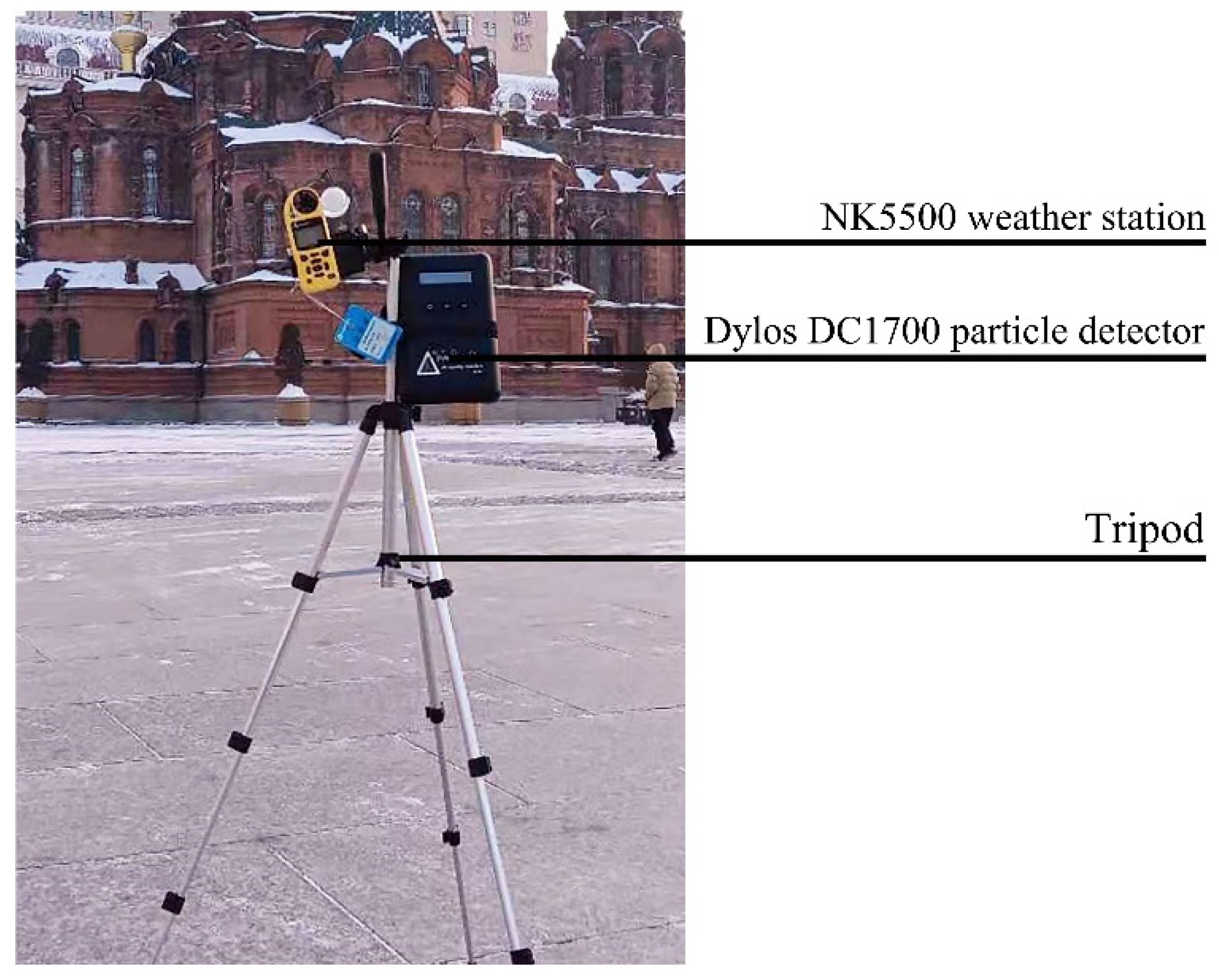
2.2. Measurement of PM2.5 and Microclimate Parameter
- (1)
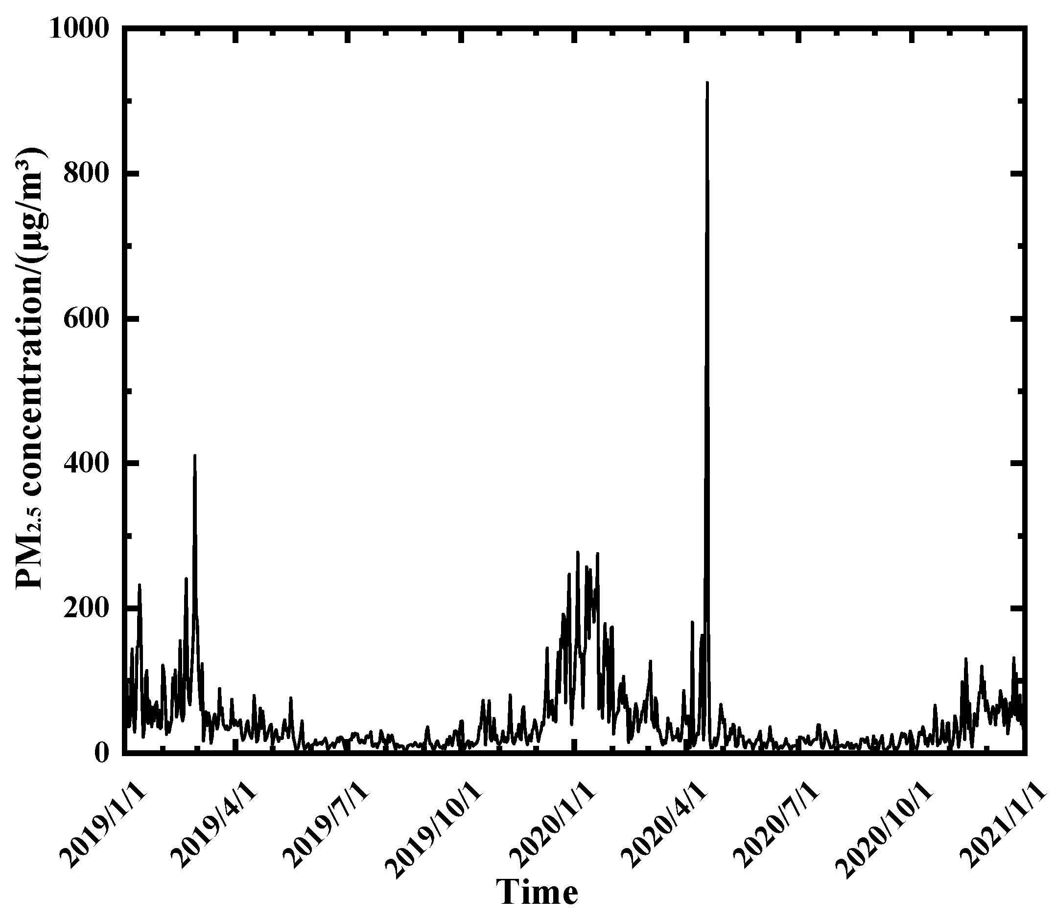
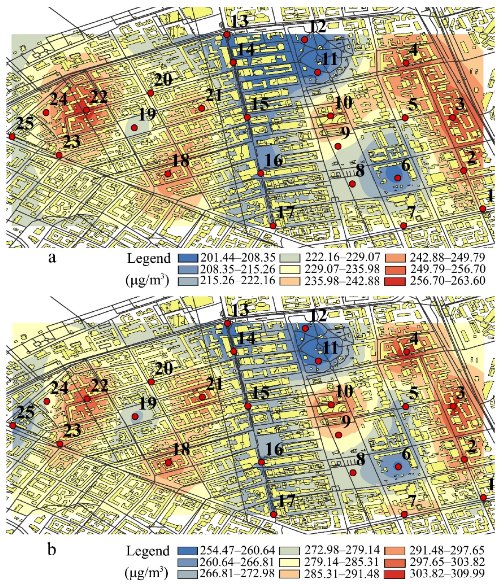
- Observe the temporal and spatial variation of PM2.5 concentration. The hourly PM2.5 concentration data of each measuring point for 21 days were collected, and then the hourly average was calculated to observe the temporal distribution characteristics of PM2.5 concentration. The PM2.5 concentration data of each measuring point at 10:00 and 22:00 for 21 days were collated, and then the mean value of these two times was calculated to observe the spatial distribution characteristics of PM2.5 concentration.
- (2)
- Observe the influence of urban microclimate on PM2.5 concentration. According to the temporal distribution characteristics of PM2.5 concentration, the typical moments when PM2.5 concentration changes were selected. The PM2.5 concentration and microclimate data at the corresponding moments of each measuring point for 21 days were collected, and then the average value at the corresponding moments was calculated to observe the influence of microclimate change on PM2.5 concentration.
- (3)
- Collect data for predictive model training and validation. The hourly PM2.5 concentration and microclimate data of each measuring point for 21 days were collected and combined with the subsequent urban morphology and other related data, finally, 12,600 sets of data were obtained, and then the training and verification of the prediction model was carried out.
2.3. Urban Morphology Parameters Analysis
2.3.1. Urban Morphology Parameters Selection and Computation
- (1)
- The parameters should significantly affect PM2.5 concentration.
- (2)
- The parameters should be easy to extract and calculate.
- (3)
- The parameters affect the design.
- (4)
- Parameter redundancy should be avoided.
2.3.2. Determination of Influence Radius of Urban Morphology Parameters
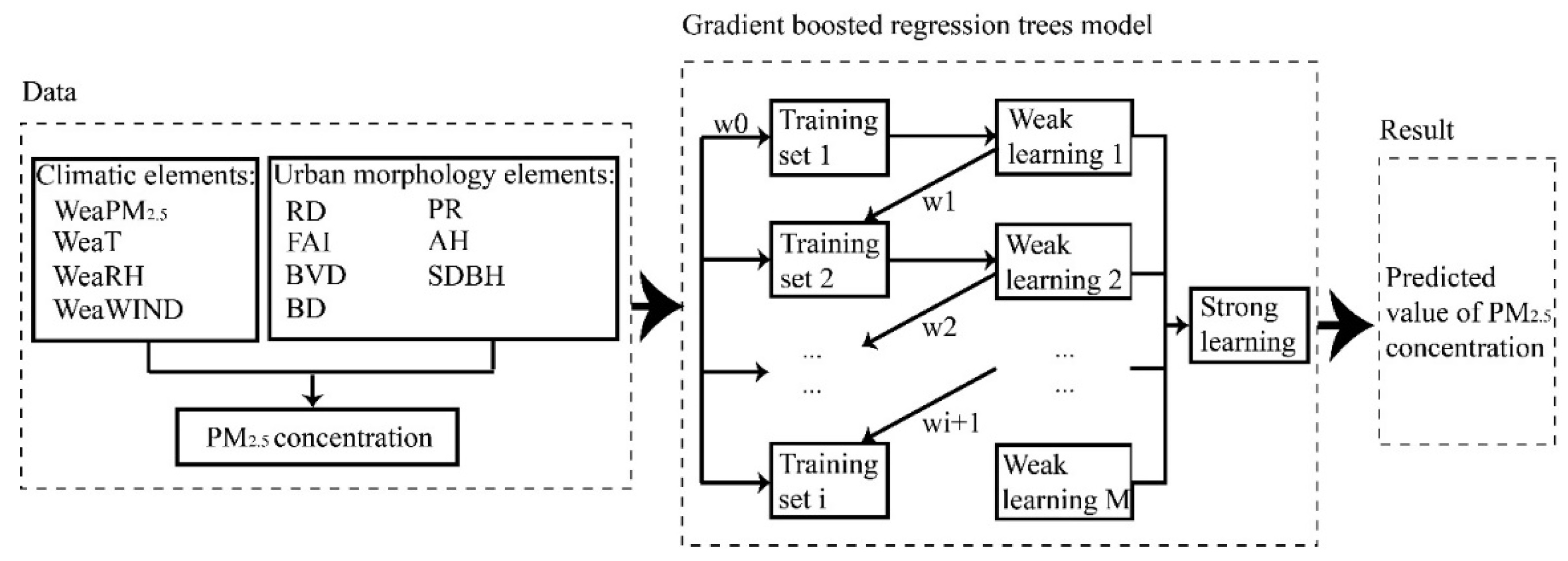
2.4. Gradient Boosted Regression (GBRT) Trees Model
2.4.1. Model Construction Principle
- (a)
- For i = 1, 2, …, N. The negative gradient direction of the loss function was calculated, and the predicted value of the model was obtained, which was used as the prediction residual. The negative gradient of the i-th training data is as follows:
- (b)
- Build a regression tree on the basis of rmi, and obtain the leaf node area Rmj of the m-th tree. Predict the leaf node area of the decision tree to obtain an approximate value of the fitting residual.
- (c)
- For j = 1, 2, …, J. Linear search is used to obtain the value in the range of leaf nodes. Minimize the loss function. The best residual fitting value of each blade is as follows:
- (d)
- Update the regression tree:
2.4.2. Model Construction and Comparative Validation
3. Results and Analysis
3.1. Temporal and Spatial Distribution of PM2.5 at Urban Block Scale
3.2. Correlation Analysis of PM2.5 Concentration and Microclimate
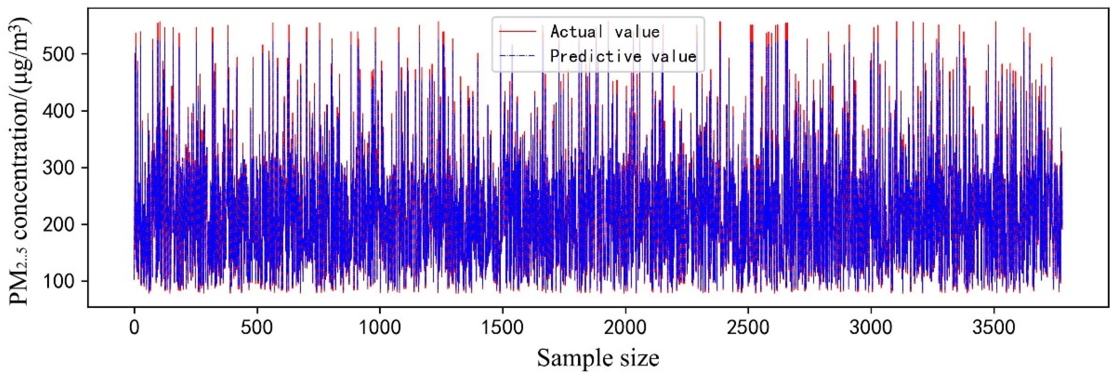
3.3. Model Analysis and Comparison of Validation Results
3.4. The Influence of Urban Spatial Morphology on PM2.5 Distribution
4. Discussion and Urban Design Recommendations
- (1)
- Horizontal layout of buildings: Building density is the urban morphology factor that has the greatest impact on PM2.5 concentration, with an impact degree of 57%; plot ratio and building volume density have an impact degree of 33% and 22% respectively. Therefore, building density parameters should be given priority.
- (2)
- Vertical layout of buildings: the influence degree of average building height and standard deviation of building height is 49% and 12% respectively, so it is necessary to make reasonable restrictions on building height. Attention should also be paid to the diversity of building height.
- (3)
- Existing buildings: it is unrealistic to demolish buildings on a large scale, but the existing urban spatial form can be improved. The impact degree of frontal area index and road density is 11% and 23% respectively. The essence of the impact of road density on PM2.5 concentration comes from automobile exhaust emissions. Based on this, removing part of the windward wall and controlling street vehicles is a practical solution.
5. Conclusions
- (1)
- There are significant temporal and spatial differences in PM2.5 concentration. The temporal difference indicates that the daily variations in PM2.5 concentration are influenced by human activities and meteorological factors. The curves of the average daily variations of PM2.5 concentration are similar, with two peaks. The spatial difference indicates that the variation in PM2.5 concentration is influenced by urban morphology factors, and PM2.5 concentration is different under different urban morphology.
- (2)
- There is a significant linear relationship between microclimate and PM2.5 concentration. Wind speed and temperature are negatively correlated with PM2.5 concentration, while humidity is positively correlated with PM2.5 concentration. However, both microclimate and PM2.5 concentrations are affected by urban morphology, indicating that urban morphology, microclimate, and PM2.5 concentration interact with each other.
- (3)
- Compared with other models, it is found that the gradient boosted regression trees (GBRT) prediction model has higher prediction accuracy and stability. The GBRT model was used to rank the influencing factors, and it was found that, except for the local PM2.5 concentration and climate data released by meteorological stations, urban morphology factors contributed significantly to the change of PM2.5 concentration. The highest influence degree is building density and average building height, followed by plot ratio, road density, building volume density, and finally standard deviation of building height and frontal area index.
Author Contributions
Funding
Institutional Review Board Statement
Informed Consent Statement
Data Availability Statement
Conflicts of Interest
Nomenclature
| RD | Road density (%) |
| FAI | Frontal area index (%) |
| BVD | Building volume density (%) |
| BD | Building density (%) |
| PR | Plot ratio |
| AH | Average building height (m) |
| SDBH | Standard deviation of building height (m) |
| T | Measured hourly temperature (°C) |
| WIND | Measured hourly wind speed (m/s) |
| RH | Measured hourly humidity (%) |
| WeaT | Hourly temperature released by the Meteorological Observatory (°C) |
| WeaWIND | Hourly wind speed released by the Meteorological Observatory (m/s) |
| WeaRH | Hourly humidity released by the Meteorological Observatory (%) |
| WeaPM2.5 | Hourly PM2.5 concentration released by the Meteorological Observatory (μg/m3) |
References
- Ma, K.; Li, C.; Xu, J.; Ren, F.; Xu, X.; Liu, C.; Niu, B.; Li, F. LncRNA Gm16410 regulates PM2.5-induced lung Endothelial-Mesenchymal Transition via the TGF-β1/Smad3/p-Smad3 pathway. Ecotoxicol. Environ. Saf. 2020, 205, 111327. [Google Scholar] [CrossRef]
- Zhang, Q.; Shen, Z.; Zhang, T.; Kong, S.; Lei, Y.; Wang, Q.; Tao, J.; Zhang, R.; Wei, P.; Wei, C.; et al. Spatial distribution and sources of winter black carbon and brown carbon in six Chinese megacities. Sci. Total Environ. 2021, 762, 143075. [Google Scholar] [CrossRef] [PubMed]
- Chen, J.; Shan, M.; Xia, J.; Jiang, Y. Effects of space heating on the pollutant emission intensities in “2+26” cities. Build. Environ. 2020, 175, 106817. [Google Scholar] [CrossRef]
- Luo, Y.; Liu, S.; Che, L.; Yu, Y. Analysis of temporal spatial distribution characteristics of PM2.5 pollution and the influential meteorological factors using Big Data in Harbin, China. J. Air Waste Manag. Assoc. 2021, 71, 964–973. [Google Scholar] [CrossRef] [PubMed]
- Liu, Z.; Jin, Y.; Jin, H. The Effects of Different Space Forms in Residential Areas on Outdoor Thermal Comfort in Severe Cold Regions of China. Int. J. Environ. Res. Public Health 2019, 16, 3960. [Google Scholar] [CrossRef] [PubMed] [Green Version]
- Fang, G.-C.; Huang, W.-J.; Chen, H.-L.; Chang, M.-C.; Chen, Y.; Huang, C.-Y. Concentrations of particulates and metallic elements in slow wind (average 1.5 m/s) in the winter season. Environ. Forensics 2017, 18, 188–196. [Google Scholar] [CrossRef]
- Yoshie, R.; Jiang, G.; Shirasawa, T.; Chung, J. CFD simulations of gas dispersion around high-rise building in non-isothermal boundary layer. J. Wind Eng. Ind. Aerodyn. 2011, 99, 279–288. [Google Scholar] [CrossRef]
- Zhang, J.; Cui, P.; Song, H. Impact of urban morphology on outdoor air temperature and microclimate optimization strategy base on Pareto optimality in Northeast China. Build. Environ. 2020, 180, 107035. [Google Scholar] [CrossRef]
- Huang, H.; Akutsu, Y.; Arai, M.; Tamura, M. A two-dimensional air quality model in an urban street canyon: Evaluation and sensitivity analysis. Atmos. Environ. 2000, 34, 689–698. [Google Scholar] [CrossRef]
- Longley, I.D.; Gallagher, M.W.; Dorsey, J.R.; Flynn, M.; Allan, J.D.; Alfarra, M.R.; Inglis, D. A case study of aerosol (4.6 nm < Dp < 10 μm) number and mass size distribution measurements in a busy street canyon in Manchester, UK. Atmos. Environ. 2003, 37, 1563–1571. [Google Scholar] [CrossRef]
- Oke, T.R. Street design and urban canopy layer climate. Energy Build. 1988, 11, 103–113. [Google Scholar] [CrossRef]
- Kaplan, H.; Dinar, N. A lagrangian dispersion model for calculating concentration distribution within a built-up domain. Atmos. Environ. 1996, 30, 4197–4207. [Google Scholar] [CrossRef]
- Chan, L.Y.; Kwok, W.S. Vertical dispersion of suspended particulates in urban area of Hong Kong. Atmos. Environ. 2000, 34, 4403–4412. [Google Scholar] [CrossRef]
- Ziomas, I.C.; Melas, D.; Zerefos, C.S.; Bais, A.F.; Paliatsos, A.G. Forecasting peak pollutant levels from meteorological variables. Atmos. Environ. 1995, 29, 3703–3711. [Google Scholar] [CrossRef]
- Kukkonen, J.; Partanen, L.; Karppinen, A.; Ruuskanen, J.; Junninen, H.; Kolehmainen, M.; Niska, H.; Dorling, S.; Chatterton, T.; Foxall, R.; et al. Extensive evaluation of neural network models for the prediction of NO2 and PM10 concentrations, compared with a deterministic modelling system and measurements in central Helsinki. Atmos. Environ. 2003, 37, 4539–4550. [Google Scholar] [CrossRef]
- McKendry, I.G. Evaluation of Artificial Neural Networks for Fine Particulate Pollution (PM10 and PM2.5) Forecasting. J. Air Waste Manag. Assoc. 2002, 52, 1096–1101. [Google Scholar] [CrossRef] [Green Version]
- Gao, Y.; Wang, Z.; Li, C.-Y.; Zheng, T.; Peng, Z.-R. Assessing neighborhood variations in ozone and PM2.5 concentrations using decision tree method. Build. Environ. 2021, 188, 107479. [Google Scholar] [CrossRef]
- Lu, W.-Z.; Wang, D. Ground-level ozone prediction by support vector machine approach with a cost-sensitive classification scheme. Sci. Total Environ. 2008, 395, 109–116. [Google Scholar] [CrossRef]
- Lu, W.-Z.; Wang, D. Learning machines: Rationale and application in ground-level ozone prediction. Appl. Soft Comput. 2014, 24, 135–141. [Google Scholar] [CrossRef]
- Wang, H.-W.; Li, X.; Wang, D.; Zhao, J.; He, H.-D.; Peng, Z.-R. Regional prediction of ground-level ozone using a hybrid sequence-to-sequence deep learning approach. J. Clean. Prod. 2019, 253, 119841. [Google Scholar] [CrossRef]
- Pach, F.P.; Abonyi, J. Association rule and decision tree based methods for fuzzy rule base generation. World Acad. Sci. Eng. Technol. 2006, 13, 45–50. [Google Scholar]
- Sachdeva, K.; Hanmandlu, M.; Kμmar, A. Real life applications of fuzzy decision tree. Int. J. Comput. Appl. 2012, 42, 24–28. [Google Scholar] [CrossRef]
- Friedman, J.H. Greedy function approximation: A gradient boosting machine. Ann. Stat. 2001, 45, 1189–1232. Available online: https://www.jstor.org/stable/2699986 (accessed on 14 January 2022). [CrossRef]
- Shi, K.; Shen, J.; Wang, L.; Ma, M.; Cui, Y. A multiscale analysis of the effect of urban expansion on PM2.5 concentrations in China: Evidence from multisource remote sensing and statistical data. Build. Environ. 2020, 174, 106778. [Google Scholar] [CrossRef]
- Liu, C.; Henderson, B.H.; Wang, D.; Yang, X.; Peng, Z.-R. A land use regression application into assessing spatial variation of intra-urban fine particulate matter (PM2.5) and nitrogen dioxide (NO2) concentrations in City of Shanghai, China. Sci. Total Environ. 2016, 565, 607–615. [Google Scholar] [CrossRef] [PubMed]
- Cheng, Y.; Yu, Q.-Q.; Liu, J.-M.; Zhu, S.; Zhang, M.; Zhang, H.; Zheng, B.; He, K.-B. Model vs. observation discrepancy in aerosol characteristics during a half-year long campaign in Northeast China: The role of biomass burning. Environ. Pollut. 2021, 269, 116167. [Google Scholar] [CrossRef] [PubMed]
- de Kok, T.M.; Driece, H.A.; Hogervorst, J.G.; Briedé, J. Toxicological assessment of ambient and traffic-related particulate matter: A review of recent studies. Mutat. Res. Mutat. Res. 2006, 613, 103–122. [Google Scholar] [CrossRef]
- Han, I.; Symanski, E.; Stock, T.H. Feasibility of using low-cost portable particle monitors for measurement of fine and coarse particulate matter in urban ambient air. J. Air Waste Manag. Assoc. 2017, 67, 330–340. [Google Scholar] [CrossRef] [Green Version]
- Liu, C.; Xu, N.; Song, J.; Hu, S. Research on visitors’ thermal sensation and space choices in an urban forest park. Acta Ecol. Sin. 2017, 37, 3561–3569. [Google Scholar] [CrossRef] [Green Version]
- Shi, Y.; Xie, X.; Fung, J.C.-H.; Ng, E. Identifying critical building morphological design factors of street-level air pollution dispersion in high-density built environment using mobile monitoring. Build. Environ. 2018, 128, 248–259. [Google Scholar] [CrossRef] [Green Version]
- Franklin, J. The elements of statistical learning: Data mining, inference and prediction. Math. Intell. 2005, 27, 83–85. [Google Scholar] [CrossRef]
- Cao, Q.; Luan, Q.; Liu, Y.; Wang, R. The effects of 2D and 3D building morphology on urban environments: A multi-scale analysis in the Beijing metropolitan region. Build. Environ. 2021, 192, 107635. [Google Scholar] [CrossRef]
- Mo, L.; Yu, X.X.; Zhao, Y.; Sun, F.B.; Mo, N.; Xia, H.L. Correlation analysis between urbanization and particle pollution in Beijing. Ecol. Environ. Sci. 2014, 23, 806–811. [Google Scholar]
- Shi, Y.; Lau, K.K.-L.; Ng, E. Developing Street-Level PM2.5 and PM10 Land Use Regression Models in High-Density Hong Kong with Urban Morphological Factors. Environ. Sci. Technol. 2016, 50, 8178–8187. [Google Scholar] [CrossRef]
- Wang, Z.; Zhong, S.; He, H.-D.; Peng, Z.-R.; Cai, M. Fine-scale variations in PM2.5 and black carbon concentrations and corresponding influential factors at an urban road intersection. Build. Environ. 2018, 141, 215–225. [Google Scholar] [CrossRef]


| Name | Usage | Technical Parameter |
|---|---|---|
| NK5500 weather station | Wind speed, Temperature, Humidity | Wind speed measurement range is 0.6–60 m/s, accuracy is ±3%, 1 inch|25 mm diameter impeller with precision axle and low-friction Zytel® bearings; Temperature measurement range is −29–70 °C, accuracy ±0.5 °C, platinum resistance temperature sensor; Humidity measurement range is 0–100%, accuracy is ±2%, polymeric capacitance humidity sensor. The measurement range is the number of particles in the air per 0.01 cubic feet of volume. The unit is μg/m3. Laser scattering method. |
| DylosDC1700 particle detector | PM2.5 concentration | Two kinds of particles of 0.5 μm and 2.5 μm can be detected. This value divided by 100 is the mass concentration of PM2.5, commonly used in China. |
| 8:00–10:00 | 12:00–15:00 | 19:00–22:00 | |
|---|---|---|---|
| WeaT (°C)/WeaRH (%)/WeaWIN (m/s)/WeaPM2.5 (μg/m3) | |||
| 1 December 2020 | −12.6/70/2.8/112.7 | −9.2/54.2/3/86.8 | −12.4/72/2.6/117 |
| 2 December 2020 | −13.1/69.3/3.3/79 | −10.2/61.8/2.9/70.3 | −13.1/74/2.5/98.5 |
| 9 December 2020 | −8.6/53.3/5.2/66 | −5.4/60.5/5.3/90 | −7.9/67.3/2.6/115 |
| 16 December 2020 | −20.6/63.7/3/78 | −16.4/51.5/3.9/65.5 | −17.9/52.8/4.5/77.8 |
| 22 December 2020 | −7/72.7/6.2/115 | −5.7/62.5/4.7/134.3 | −13.1/88.5/0.7/147.3 |
| 24 December 2020 | −17/71.7/2.5/114.7 | −14.1/59.5/2.6/139 | −19.4/86/0.73/149.3 |
| 1 January 2021 | −23.2/72/2.4/62.3 | −18.6/57.5/2.5/95 | −22.8/65/1.6/83.5 |
| 4 January 2021 | −20.9/65.7/3.3/77.3 | −17.4/55.3/2.9/92.3 | −20.9/73.3/2.2/65.5 |
| 5 January 2021 | −21.5/65.7/2.7/56.3 | −17.5/55.3/3/77.5 | −19.8/64.8/2.4/99 |
| 9 January 2021 | −22.7/68/2.4/99 | −17.9/54/3.2/155.8 | −19.8/65.5/2/135.5 |
| 11 January 2021 | −15.2/67.3/3.7/101.3 | −12.1/57/3.4/90.3 | −15.1/78.8/1.3/74.5 |
| 12 January 2021 | −15.7/84.3/1.6/102.3 | −8.9/73.8/2.7/96.5 | −8.6/92.5/2/91.3 |
| 13 January 2021 | −17/79.3/4/83.7 | −14.3/70.8/3.8/104.5 | −16.4/84/1.9/96.8 |
| 14 January 2021 | −19.3/75.7/2.3/112.3 | −16.4/66.3/1.9/99.3 | −18.7/77.5/1.4/53.8 |
| 20 January 2021 | −13.9/83/1.7/68 | −4.2/85.5/4.8/99 | −6.4/83.3/2.9/68.8 |
| 21 January 2021 | −15.3/82.7/1.2/107.7 | −8.9/56.8/3/198.8 | −15.9/71.3/2.4/70 |
| 23 January 2021 | −16/77/1/142.3 | −7.6/52.8/1.3/162.3 | −13.8/80.5/1.3/214.5 |
| 24 January 2021 | −11.2/83.3/0.7/263.3 | −2.5/56.3/1.3/210.5 | −13.8/88.3/1.1/62 |
| 8 February 2021 | −10.5/78/2.1/118 | −3.2/63/2.3/116 | −14.5/82/2.4/121 |
| 14 February 2021 | −8.4/62/3.2/89 | −2.3/54/3.6/78 | −11.6/76/3.5/95 |
| 15 February 2021 | −7.6/79/2.8/91 | −1.9/69/3.4/88 | −10.8/86/2.6/111 |
| Urban Morphology Factor | Unit | Equation of Calculation | Theoretical Meaning |
|---|---|---|---|
| RD | % | Traffic pollution intensity | |
| FAI | % | The blocking effect of the buildings in the plot on the airflow | |
| BVD | % | The spatial density of the buildings in the plot | |
| BD | % | The level of building density in the horizontal direction within the plot | |
| PR | - | The overall volume and development intensity of the buildings in the plot | |
| AH | m | Vertical building development intensity | |
| SDBH | - | The degree of difference and dislocation of the vertical building height within the plot |
| Urban Morphology Factor | RD | FAI | BVD | BD | PR | AH | SDBH |
|---|---|---|---|---|---|---|---|
| No.1: R2/sig (50 m) | 0.696/0.0 | 0.633/0.5 | 0.766/0.0 | 0.580/0.0 | 0.635/0.0 | 0.663/0.09 | 0.731/0.06 |
| No.2: R2/sig (100 m) | 0.754/0.0 | 0.685/0.0 | 0.829/0.0 | 0.628/0.0 | 0.605/0.0 | 0.718/0.0 | 0.792/0.0 |
| No.3: R2/sig (200 m) | 0.792/0.0 | 0.720/0.01 | 0.87/0.0 | 0.660/0.02 | 0.794/0.0 | 0.754/0.0 | 0.890/0.0 |
| No.4: R2/sig (300 m) | 0.895/0.0 | 0.814/0.0 | 0.915/0.03 | 0.846/0.0 | 0.750/0.0 | 0.752/0.02 | 0.840/0.0 |
| No.5: R2/sig (400 m) | 0.625/0.0 | 0.568/0.0 | 0.688/0.0 | 0.521/0.0 | 0.753/0.0 | 0.795/0.0 | 0.656/0.0 |
| No.6: R2/sig (500 m) | 0.533/0.1 | 0.485/0.0 | 0.586/0.0 | 0.444/0.0 | 0.640/0.0 | 0.852/0.01 | 0.560/0.2 |
| GBRT | MLR | RF | DT | |
|---|---|---|---|---|
| MAE (μg/m3) | 1.452 | 3.690 | 1.631 | 2.308 |
| MSE (μg/m3) | 3.246 | 8.872 | 4.285 | 5.197 |
| R2 | 0.978 | 0.791 | 0.966 | 0.894 |
| Model | Advantage | Disadvantage | ||
|---|---|---|---|---|
| Empirical model | Linear regression model | Land use regression (LUR) | Fast calculation speed | Failed to capture the nonlinear relationships |
| Multiple linear regression (MLR) | Fast calculation speed | Failed to capture the nonlinear relationships | ||
| Machine learning method | Decision tree (DT) | Capture the nonlinear relationships | Low prediction accuracy | |
| Random forest (RF) | Capture the nonlinear relationships; Rank the influencing variables based on their importance | - | ||
| Gradient boosted regression trees (GBRT) | Capture the nonlinear relationships; Rank the influencing variables based on their importance | - | ||
| Support vector machine (SVM) | Capture the nonlinear relationships | Cannot rank the influencing variables based on their importance | ||
| Multi-layer perceptron | Capture the nonlinear relationships | Cannot rank the influencing variables based on their importance | ||
| Sequence learning | Capture the nonlinear relationships | Cannot rank the influencing variables based on their importance | ||
| Deterministic model | - | Weather research and forecasting (WRF) | Applicable to macroscale | Limited the analysis of air quality at microscales |
| Community multiscale air quality (CMAQ) | Applicable to macroscal | Limited the analysis of air quality at microscales |
Publisher’s Note: MDPI stays neutral with regard to jurisdictional claims in published maps and institutional affiliations. |
© 2022 by the authors. Licensee MDPI, Basel, Switzerland. This article is an open access article distributed under the terms and conditions of the Creative Commons Attribution (CC BY) license (https://creativecommons.org/licenses/by/4.0/).
Share and Cite
Cui, P.; Dai, C.; Zhang, J.; Li, T. Assessing the Effects of Urban Morphology Parameters on PM2.5 Distribution in Northeast China Based on Gradient Boosted Regression Trees Method. Sustainability 2022, 14, 2618. https://doi.org/10.3390/su14052618
Cui P, Dai C, Zhang J, Li T. Assessing the Effects of Urban Morphology Parameters on PM2.5 Distribution in Northeast China Based on Gradient Boosted Regression Trees Method. Sustainability. 2022; 14(5):2618. https://doi.org/10.3390/su14052618
Chicago/Turabian StyleCui, Peng, Chunyu Dai, Jun Zhang, and Tingting Li. 2022. "Assessing the Effects of Urban Morphology Parameters on PM2.5 Distribution in Northeast China Based on Gradient Boosted Regression Trees Method" Sustainability 14, no. 5: 2618. https://doi.org/10.3390/su14052618
APA StyleCui, P., Dai, C., Zhang, J., & Li, T. (2022). Assessing the Effects of Urban Morphology Parameters on PM2.5 Distribution in Northeast China Based on Gradient Boosted Regression Trees Method. Sustainability, 14(5), 2618. https://doi.org/10.3390/su14052618