Predicting Demand for Shared E-Scooter Using Community Structure and Deep Learning Method

Abstract

The shared e-scooter is a popular and user-convenient mode of transportation, owing to the free-floating manner of its service. The free-floating service has the advantage of offering pick-up and drop-off anywhere, but has the disadvantage of being unavailable at the desired time and place because it is spread across the service area. To improve the level of service, relocation strategies for shared e-scooters are needed, and it is important to predict the demand for their use within a given area. Therefore, this study aimed to develop a demand prediction model for the use of shared e-scooters. The temporal scope was selected as October 2020, when the demand for e-scooter use was the highest in 2020, and the spatial scope was selected as Seocho and Gangnam, where shared e-scooter services were first introduced and most frequently used in Seoul, Korea. The spatial unit for the analysis was set as a 200 m square grid, and the hourly demand for each grid was aggregated based on e-scooter trip data. Prior to predicting the demand, the spatial area was clustered into five communities using the community structure method. The demand prediction model was developed based on long short-term memory (LSTM) and the prediction results according to the activation function were compared. As a result, the model employing the exponential linear unit (ELU) and the hyperbolic tangent (tanh) as the activation function produced good predictions regarding peak time demands and off-peak demands, respectively. This study presents a methodology for the efficient analysis of the wider spatial area of e-scooters.

1. Introduction

The shared e-scooter service (e.g., Lime and Bird) first appeared in the United States in 2017 [1,2,3,4]. Since then, it has been introduced in many cities around the world in order to reduce traffic congestion and air pollution, and to enhance community relationships as well as resilience in urban mobility, which is an important asset for sustainable urban mobility [5]. In addition, during the COVID-19 pandemic, the use of shared e-scooters as an alternative to public transportation for short-distance travel is increasing [6]. In Seoul, Korea, the shared e-scooter service (e.g., Kickgoing) began in 2018 and, as of August 2020, there are 16 services sharing more than 36,000 e-scooters in the city [7]. In Korea, shared e-scooter services are very popular due to user convenience, as the serviced is available in a free-floating manner without a fixed station, unlike previous shared mobilities such as bike sharing and car sharing. The free-floating nature of the service has the advantage that users can drop off the e-scooters in the desired area; however, there are disadvantages because this can cause urban problems such as traffic accidents and impaired pedestrian environment due to reckless service operations [8,9]. In addition, there is a problem that the e-scooters are spread across the service area, so that they may not be available in the desired area. To solve this problem, it is necessary to relocate the e-scooters in order to meet the demand for use.

The relocation method is simple: move e-scooters from areas where there is no demand for use to areas where demand is expected to be high. The key to this simple process is to determine whether a certain area is in high demand or not. In other words, to predict the demand for use in the area. Therefore, this study aims to predict the demand for shared e-scooters.

This study is organized as follows. Section 2 reviews studies on the demand for the use of e-scooters. Section 3 explains how data were collected and processed, how the unit of analysis for demand was set, and what methodologies were used to predict the demand. In Section 4, we present the results of predicting demand based on the analysis unit set out in Section 3. Finally, in Section 5, we briefly summarize the results of this study, mention the implications and limitations of the study, and suggest future research directions.

2. Literature Review

Previous studies using shared e-scooter trip data analyzed simple travel characteristics [2,4,10,11] and identified factors affecting demand (e.g., gender, age, education level, income level, population density, employment density, student ratio, land-use diversity, residential type, distance from the city center, public transportation accessibility, bicycle road, and intersection density) [12,13,14,15]. Recently, a study [16] on predicting demand using deep learning methods was also performed. There have been other studies suggesting ways to improve the legal system [1,8,17,18], promoting ways to enhance inclusiveness such as gender equity [19], selecting the location of battery charging systems [20], and estimating travel purpose [21]. Furthermore, a teaching concept differentiated by education level was introduced to improve the understanding of electric mobility including e-scooter [22].

Liu et al. [2] evaluated travel patterns by analyzing shared e-scooter trip data in Indianapolis from September to November 2018. Of the total trips, 60% and 65% were shorter than 10 min and less than 1 mile, respectively. Looking at the usage distribution by time period, the usage increases from 11:00 to 21:00, which is different from the morning and afternoon peak distributions of typical transportation modes. McKenzie [4] compared the usage patterns of scooter-share and bike-share in Washington, D.C. from June to August 2018. Users of bike-share used the service a great deal in the morning and afternoon on weekdays, while casual users of bike-share and scooter-share did not show a special peak pattern. Looking at the spatial distribution, it was found that bike-shares were more concentrated in the city center than scooter-shares. Zou et al. [10] used e-scooter trip data in Washington, D.C. from March to April 2019. The average trip duration was 14 min, and the average travel speed was 4.5 mph. On weekdays, the trip volume increased rapidly from 8:00, at rush hour, while it increased from 9:00 on weekends. Looking at the spatial distribution, it was found that e-scooters are mainly used in commercial areas in the center of the city and are also partially used in parks and the riverside. Raptopoulou et al. [11] surveyed the attitudes and behaviors of 271 users toward e-scooters in Thessaloniki, Greece. Most users used the service for less than once a month, and used it for short durations of less than 10 min. In addition, more than half of the users used a combination of other means of transportation and e-scooters less than once a week. The e-scooters were mainly used for leisure or shopping purposes, and they were not much used for commuting. In addition, bad driving behavior, traffic congestion, and weather conditions were considered important factors with respect to e-scooter use.

Bai and Jiao [12] compared the usage pattern of dockless e-scooters in Austin, Texas, and Minneapolis, Minnesota, in August and November 2018. Dockless e-scooters were used for longer in Minneapolis than in Austin; the trip duration and distance were longer by 4 min and 0.4 miles, respectively. In both cities, e-scooters were mainly used in the city center and near the university campuses. In addition, the factors affecting usage were explored using a negative binomial regression model. As a result of the analysis, it was shown that factors linked to the urban built environment, such as distance to city center, transit accessibility, land use diversity, and various facility areas (e.g., residential, commercial, office, transportation facility, and so on), affected average daily ridership. Caspi et al. [13] used shared e-scooter trip records in Austin, Texas, from August 2018 to February 2019. Of the total number of trips, 18% occurred in the afternoon (16:00 to 19:00). Spatially, the service was mainly used in the city center and near the University of Austin. By estimating a spatial lag model (SLM) and a spatial durbin model (SDM), the influencing factors were identified on the basis of a 200 m square grid. As a result of the analysis, land use variables (e.g., residential, commercial, educational, and recreation land use area ratio), transportation facility variables (e.g., bikeways in cell, bus stops in cell, intersection density), and demographic variables (e.g., student ratio, employment density) were found to affect e-scooter trip generation. In addition, geographically weighted regression (GWR) models were developed to examine the influencing factors for each cell. Residential land use area ratio had a greater influence in the west and the south of the city center in Austin, and median annual income and student ratio were determined to have a negative influence on trips in the west. Hosseinzadeh et al. [14] investigated the relationship between the density of e-scooter trips and characteristics of sustainable urban development in Louisville, Kentucky, from August 2018 to February 2020. Spatial factors were identified by developing a generalized additive modeling (GAM) based on 159 traffic analysis zones (TAZ). The results of the models for all trips and peak-time trips demonstrated that land use affects e-scooter trip density. Regarding the urbanism score, almost all combinations of walk, bike, and transit scores were found to be significant in both models. Lee et al. [15] developed a multivariate log-linear regression model to estimate e-scooter trips based on TAZ. The trip data was collected from a pilot program in Portland conducted from July to November 2019. It was found that sociodemographic attributes such as population density, 20–40 age range, labor force participation, health insurance coverage, and income affect the demand for e-scooter sharing systems.

In addition, the studies in which models for predicting demand through deep learning approaches were developed were performed mainly on shared bicycles. There are two approaches in building models: using deep learning combined with other machine learning methods [23,24,25,26], and using deep learning alone [27,28,29,30].

Chang et al. [23] predicted the overall city-wide demand of shared bicycles by integrating AIS (Artificial Immune Systems), one of the optimization techniques, and ANN (Artificial Neural Network). The process steps of the proposed model consist of cell generation, antibody generation, and antibody adaptation, and ANN is used in the cell generation step. To consider temporal features, dummy variables for holidays and weekends were added, and variables related to weather such as temperature and wind speed were used. Xu et al. [24] proposed a SOM-RT technique that integrates a self-organizing mapping network (SOM) and a regression tree (RT). The SOM layer clusters the historical shared bicycle data with similar characteristics, and based on the clusters, RT predicts the demand. Zhou et al. [25] conducted the bicycle demand prediction in two stages. In the first step, a variety of models, like MLP (multilayer perceptron), SVM (support vector machine), and linear regression model were used and compared to predict the city-wide bicycle demand. After that, in the second step, the demand of each station was predicted based on the city-wide demand predicted earlier through the Markov chain. It was found that the linear regression model was most suitable for forecasting city-wide bicycle demand. However, there was a limitation in these studies in that temporal dependency was not directly reflected, being processed through a dummy variable on the day of the week. Yang et al. [26] derived variables affecting the demand of bicycles using the XGBoost (extreme gradient boosting) algorithm. Unlike other studies, the relationship between bicycle stations, including demand, was represented by a graph, and graph structure variables such as betweenness centrality of each node were constructed. As a result, the importance of the variables related to the graph structure was higher than the weather-related variables used in previous studies. Using the selected variables, XGBoost, MLP, and long short-term memory (LSTM) methods were used to predict the demand of each station, and LSTM had the best performance among them.

Most of the studies predicting the demand for bicycle use based on deep learning have used LSTM. These can be divided into studies using only the LSTM layer and studies using LSTM integrated with different layers. First, Pan et al. [27] and Xu et al. [28] used LSTM layers alone; Pan et al. [27] predicted the demand of fixed bicycle stations, whereas Xu et al. [28] predicted the demand of a free-floating bicycle. Since free-floating services do not occur in a fixed place, Xu et al. [28] predicted the demand by aggregating the demand for bicycles using TAZ. Meanwhile, Ai et al. [29] and Lin et al. [30] combined the LSTM layer, the convolution layer, and the graph-convolution layer, respectively. These layers are often used to capture spatial features. Ai et al. [29] predicted the demand for free-floating bicycles. After dividing the city to be analyzed into 7 × 7 grids with a size of 4 km, the demand for each grid was predicted, spatial features were captured through a convolution layer, and temporal dependency was then reflected through an LSTM layer. However, since the grid size was large, at 4 km, the prediction had limitations with respect to capturing detailed spatial features. Lin et al. [30] predicted the demand at fixed bicycle stations, and similar to the Yang et al. [26] study mentioned above, the relationship between stations was represented in a graph so that the characteristics of the nearby bicycle station could be reflected. However, these studies did not consider variables (weather, day of the week, etc.) other than demand.

Looking at the activation functions, Ai et al. [29] used hyperbolic tangent (tanh), Chang et al. [23] and Pan et al. [27] used sigmoid, Lin et al. [30] used ReLU, and Xu et al. [28] used sigmoid and tanh. In addition, some studies [23,24,25,26,27,28] have applied external factors (e.g., weather, land use, and so on) as well as previous timestep demand as input data.

Unlike previous studies predicting bicycle demand, Ham et al. [16] recently performed a study that aimed to establish a methodology for predicting e-scooters demand using e-scooter sharing service usage data collected from 8 August 2019 to 10 September 2019 in Gwangjin-gu, Seoul, Korea. A spatial unit was constructed by dividing the analysis area into a 250 m square grid, considering walking speed and app execution time. The demand covered both the actual demand and the “unmet demand” that was not actually used even though the app was executed. An encoder–recurrent neural network–decoder (ERD) framework was constructed to predict demand by time-period, including unmet demand. The prediction model included long short-term memory (LSTM) and gated recurrent unit (GRU), and the activation functions were a sigmoid, a rectified linear unit (ReLU), and an exponential linear unit (ELU). The prediction model with the LSTM cell and ReLU as the activation function, and the learning rate of 0.0010 showing the best results.

On the other hand, Zhang et al. [31], who predicted dynamic urban traffic flow, considered temporal effects in the same way as other studies, but suggested ST-GAN (Spatial-Temporal Generative Adversarial Network) based on GAN rather than LSTM for time series prediction. Sigmoid, tanh, and sigmoid were used as activation functions of the last layer of Discriminator, Generator, and Encoder composing ST-GAN, respectively, and Leaky ReLU was used for the other layers.

Summarizing the previous studies, most of the studies related to the demand for shared e-scooter used a statistical model to explain the factors affecting trip generation. Those studies that predicted the demand for use by means of deep learning methods were mainly conducted for shared bicycle services, and Ham et al. [16] was the only study that predicted the demand for shared e-scooters. This study, similar to Ham et al. [16], tried to predict the demand for shared e-scooters using the deep learning approach. Unlike the previous study, the study was conducted on a small scale with 252 grids; moreover, in this study, the demand for use was predicted for 1164 grids in Seocho and Gangnam, which are the most used areas in Seoul. For efficiency of analysis, the concept of community structure, a methodology for simplifying complex networks by clustering, was applied. Community structure was proposed by Girvan and Newman [32], and suitable methodologies for large-scale networks are continuously being studied [33,34]. Community structure methodologies will be dealt with in detail in Section 3. Zhang et al. [35] applied the community structure methodology to the transportation field. They presented a methodology for covering the maximum service area with the minimum number of shared bikes and allocating bikes so that the maximum number of users can use them. The community structure was applied to 24 TAZ of Sioux Falls, South Dakota and 100 TAZ of Singapore. Both cities were grouped into five TAZ, and allocation positions were selected at which to place the shared bikes. In other words, the maximum efficiency was derived with the minimum cost through the community structure. Therefore, in this study, the demand for use is predicted by applying the community structure method to a large-scale network of 1164 TAZ. We think that community structure is a key process for the efficient conclusion of the e-scooter relocation problem.

3. Data and Methodology

This section explains the data used in this study, the community structure method for establishing a service cluster, and the LSTM for predicting the demand for e-scooters. The equations of the community structure and LSTM are cited from Blondel et al. [34] and Olah [36], respectively.

3.1. Data Collection

Trip data of XingXing, a shared e-scooter service of the PUMP Corporation, were used in this study. XingXing started in Seocho and Gangnam in June 2019 and as of July 2021 is in service in more than 60 cities. The data include the rental date and time, rental location, return date and time, return location, trip duration, and trip distance. The temporal and spatial scopes of the data were selected as October 2020 and Seocho and Gangnam, respectively, by reviewing the trip frequency. The total number of trips excluding errors was 713,622 trips, of which Seocho and Gangnam accounted for 224,096 trips, thus accounting for approximately 31% of the total trips. The data errors include location information omission, trip duration less than 20 s (company policy), trip distance of 0 m, and average speed exceeding 25 km/h (maximum speed limit of vehicle). Seocho and Gangnam have 41 subway stations, being one of the central business districts (CBD) in Seoul.

Since the shared e-scooter service is a free-floating service, it was necessary to set the spatial unit for efficient analysis. In this study, the spatial unit was set as a square grid. Following Caspi et al. [13], the size of the square grid was 200 m. Seocho and Gangnam are composed of approximately 2300 square grids. The free-floating service is available anywhere in the service area, excluding some areas such as private areas, parks, and schools, as shown in the left-hand image of Figure 1. Therefore, these areas are assumed to be unavailable areas, where there is no pick-up and drop-off. As a result, 1164 square grids were set as the analysis area, as shown in the right-hand image of Figure 1.

This study aimed to predict the hourly demand for each square grid. The hourly demand is the aggregated pick-up demand for 1164 square grids and 744 time windows (31 days × 24 h). The explanatory variables include time variables and weather variables. For the weather variables, temperature and wind speed were measured using the automatic weather system (AWS) of the Meteorological Data Open Portal of the Korea Meteorological Administration. Variables are described in

Table 1. Explanation of variables.

Variables		Type	Explanation
Hourly demand (Pick-up)		Numeric	The number of hourly demand (pick-up)
Time variables	Weekday	Binary	1: a weekday, 0: otherwise
	Weekend	Binary	1: a weekend, 0: otherwise
	Hour of day	Numeric	Time window
Weather variables	Temperature	Numeric	Temperature in Celsius
	Wind speed	Numeric	Wind speed in meter per second

.

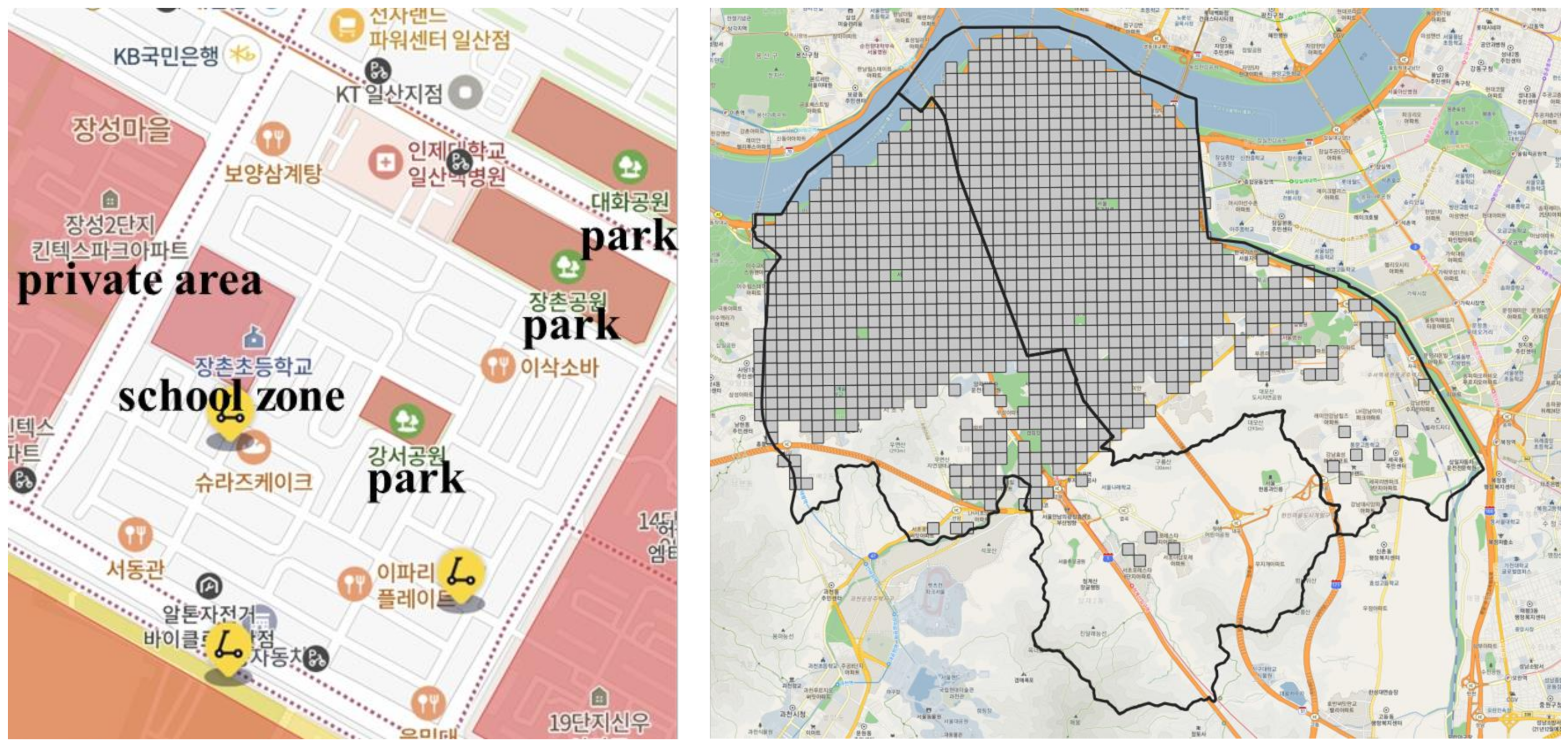
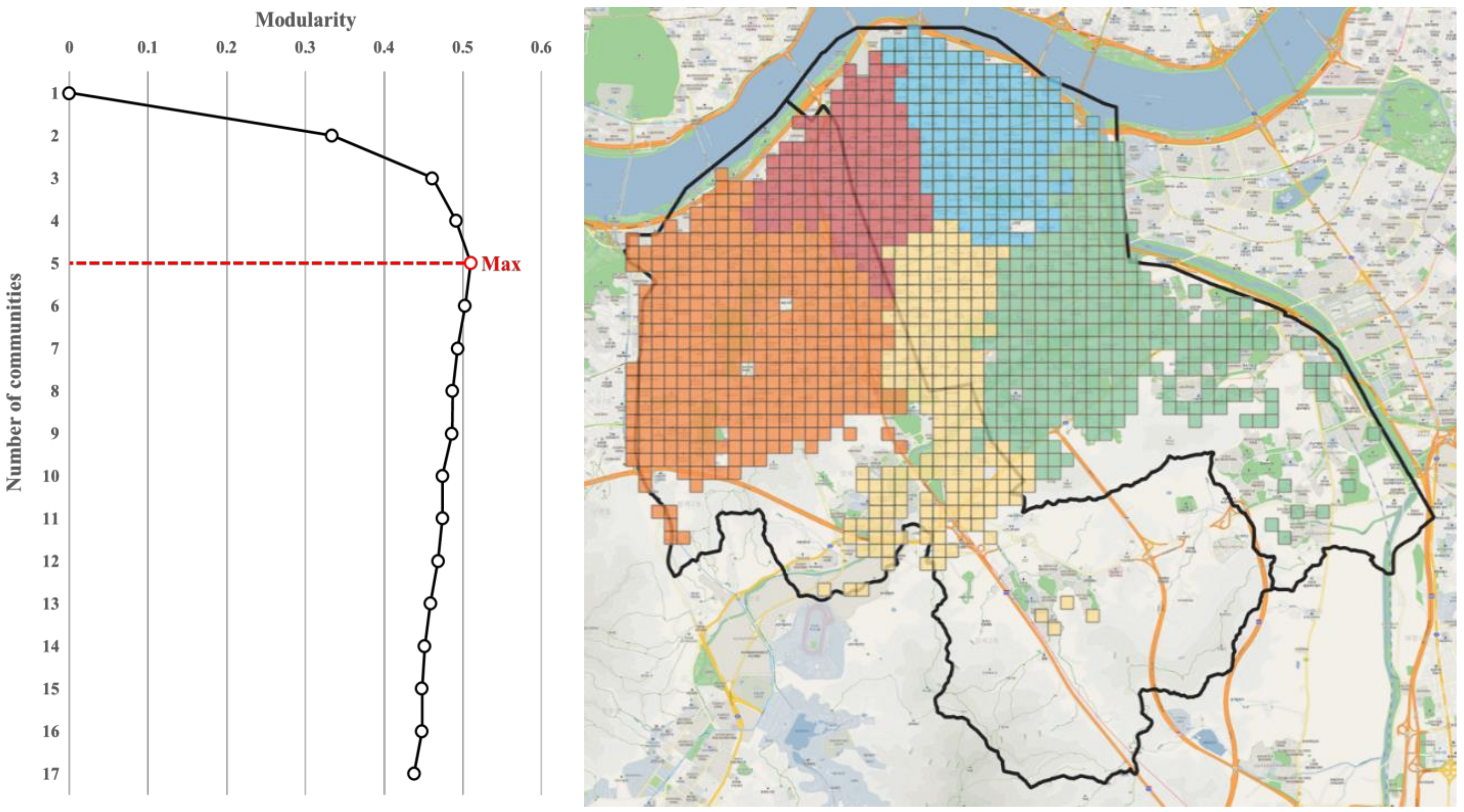
3.2. Community Structure

Networks are very complicated in the real world. Complex networks have various characteristics, and many researchers have analyzed complex networks: transportation networks consist of nodes and links, neural networks are connections between neurons, and social networks are relationships between people [37,38,39,40].

A network consists of a vertex and an edge: a vertex and edge mean node and link, respectively, in this study. Since the network in the real world is too complicated, consisting of many nodes and links, it is necessary to simplify it. The community structure developed by Girvan and Newman is a representative method for simplifying networks [32]. The community structure maximizes modularity and clusters complex networks. Modularity means the connectivity of the clustered network, and quantitatively indicates whether a meaningful community is formed. The modularity has a value from −1 to 1, and the community can be designated as well divided if the value is larger [41]. Modularity Q is calculated as shown in Equation (1):

$$Q=\frac{1}{2m}{{\displaystyle \sum }}_{ij}\left[a_{ij}-\frac{k_i{k}_j}{2m}\right]\delta \left(c_i,c_j\right)$$

(1)

where m is the total number of links in the network, $a_{ij}$ is the number of links between node i and j; the number of links indicates the traffic volume in this study. $k_i$ and $k_j$ are the degree of the nodes i and j, respectively. The degree of the node is the number of connected links of the node, which corresponds to the pick-up and drop-off demands of the node in this paper. $c_i$ and $c_j$ are the communities to which nodes i and j belong, respectively. $\delta \left(c_i,c_j\right)$ is the relationship function of $c_i$ and $c_j$. If nodes i and j belong to the same community, that is $c_i$ = $c_j$, then $\delta \left(c_i,c_j\right)$ = 1; otherwise, $\delta \left(c_i,c_j\right)$ = 0.

Equation (1) calculates modularity in terms of node and can be expressed as Equation (2) in terms of community.

$$Q={\displaystyle \sum }_l^n\left(e_{ll}-a_l^2\right)$$

(2)

where n (l = 1, 2, …, l, …, l′, …, n) is the total number of the community. $e_{l{l}^{\prime }}$ is the ratio of the number of links between communities to the total number of links in the network, according to Equation (3), and $a_l$ is shown in Equation (4):

$$e_{l{l}^{\prime }}=\frac{1}{2m}{{\displaystyle \sum }}_{i\in c_i}{{\displaystyle \sum }}_{j\in c_j}{a}_{ij}$$

(3)

$$a_l={{\displaystyle \sum }}_{l^{\prime }}^n{e}_{l{l}^{\prime }}$$

(4)

Representative algorithms of the community structure include the Girvan–Newman algorithm, FN algorithm, greedy algorithm, and Louvain algorithm [32,33,34,42]. The Girvan–Newman algorithm uses betweenness centrality, which indicates how many nodes k exist on the shortest path from node i to node j. The modularity is calculated by removing the node with the highest betweenness centrality in order. This method has the disadvantage that it takes a long time to calculate [32]. The F-N algorithm is a bottom-up algorithm that combines similar nodes and communities [33]. It has the advantage of fast calculation time, but there is the disadvantage that the weight of the link cannot be reflected [35]. The greedy algorithm also improves the calculation time, but it has weaknesses in performance optimization, such as creating a super-community [42]. In addition to the algorithms described above, Ahn et al. [43] studied the link community, which is developed by calculating the similarity between links. Since the link community forms a community based on links, the same node can belong to several communities.

This study adopted the Louvain algorithm, which addresses the problems of the previous algorithm such that calculation was fast, and the community was divided by reflecting the link weight [34]. The algorithm consists of two phases. In the first phase, a node is moved from the previous community to another community, and modularity is calculated repeatedly. Then, the move with the largest modularity is chosen. Another node is moved just as in the previous step, and this movement is repeated until modularity does not change. At this point, the change of modularity appears as shown in Equation (5):

$$\Delta Q=\left[\frac{{{\displaystyle \sum }}_{in}+2k_{i,in}}{2m}-{\left(\frac{{{\displaystyle \sum }}_{tot}+k_i}{2m}\right)}^2\right]-\left[\frac{{\sum }_{in}}{2m}-{\left(\frac{{\sum }_{tot}}{2m}\right)}^2-{\left(\frac{k_i}{2m}\right)}^2\right]$$

(5)

where ${\sum }_{in}$ is the sum of the weight of the links within the community to which node i belongs. ${\sum }_{tot}$ is the sum of the weight of the links of the community to which node i belongs. In this study, ${\sum }_{in}$ and ${\sum }_{tot}$ refer to the internal traffic volume of the community and the total traffic volume of the community, respectively. $k_{i,in}$ is the degree of connection between node i and the other nodes within the community to which node i belongs, i.e., the pick-up and drop-off demands at node I within the community.

In the second phase, the community created in phase 1 is combined into one block, and the links between communities are combined into one link to simplify the network. The simplified network is again applied to the algorithm of phase 1. This process is repeated after phase 2, until there is no more change in phase 1. The Louvain algorithm can produce different results depending on the node it starts from. However, according to a study by Blondel et al. [34], the starting node has no significant effect on modularity, and it can only affect computation time.

3.3. Long Short-Term Memory (LSTM)

LSTM is based on recurrent neural network (RNN). RNN has a structure that repeats itself by receiving information from the previous step and deriving the result of the next step. This structure can process sequence-type data using internal memory, so it is used in various fields such as speech recognition, language modeling, and translation [44,45,46]. RNN has an additional storage space called gated state or gated memory, and LSTM was developed by applying it.

LSTM was introduced in Hochreiter and Schmidhuber [47] by supplementing the problem of RNN, the difficulty in predicting long periods. LSTM has several advantages compared to the other time series model. First, it has excellent predictive power for nonlinear relationships of time series data [28,48,49]. Next, it is possible to prevent the problem of abruptly disappearing or increasing slope values [28,47,50,51].

The core of LSTM is the cell state. The cell state is the part that receives the information of the previous step. LSTM has three gates that control the cell state. The first gate is a forget gate that determines which information of the cell state to discard. The activation value of the forget value ($f_t$) is calculated by applying the activation function ($\sigma$) to the output of the previous time interval ($h_{t-1}$) and the time series data of the current time interval ($x_t$). $f_t$ can be expressed as shown in Equation (6):

$$f_t=\sigma \left(W_f\cdot \left[h_{t-1},x_t\right]+b_f\right)$$

(6)

The activation function determines how much information is transmitted, and there are sigmoid, ReLU, ELU, tanh, and so on. The major activation functions are given by Equations (7)–(10):

$$sigmoid\left(x\right)=\frac{1}{1+e^{-x}}$$

(7)

$$ReLU\left(x\right)=\left\{\begin{array}{c}x \left(x\ge 0\right)\\ 0 (x<0)\end{array}\right.$$

(8)

$$ELU\left(\alpha ,x\right)=\left\{\begin{array}{c}x (x>0)\\ \alpha \left(e^x-1\right) \left(x\le 0\right)\end{array}\right.$$

(9)

$$tanh\left(x\right)=\frac{\left(e^x-e^{-x}\right)}{\left(e^x+e^{-x}\right)}$$

(10)

The second gate is an input gate that determines which information to store among the information coming into the cell state. The activation value of the input gate ($i_t$) is calculated using the activation function ($\sigma$), and a candidate value (${\tilde{C}}_t$) is generated using the hyperbolic tangent function. $i_t$ and ${\tilde{C}}_t$ appear as shown in Equations (11) and (12):

$$i_t=\sigma \left(W_i\cdot \left[h_{t-1},x_t\right]+b_i\right)$$

(11)

$${\tilde{C}}_t=tanh\left(W_C\cdot \left[h_{t-1},x_t\right]+b_C\right)$$

(12)

Then, a new cell state ($C_t$) is generated by combining the results of the forget gate and the input gate. $C_t$ appears as in Equation (13):

$$C_t=f_t\ast C_{t-1}+i_t\ast {\tilde{C}}_t$$

(13)

The last gate is an output gate that predicts the output of the current time interval ($h_t$) by combining the activation value of output gate ($o_t$) and $C_t$. $o_t$ is calculated using the activation function ($\sigma$), just as with $f_t$ and $i_t$. $o_t$ and $h_t$ are shown as Equations (14) and (15):

$$o_t=\sigma \left(W_o\cdot \left[h_{t-1},x_t\right]+b_o\right)$$

(14)

$$h_t=o_t\ast tanh\left(C_t\right)$$

(15)

We predicted the next hourly demand with the previous 24 h demand to reflect the temporal demand pattern. For hourly demand prediction, the entire data set was divided into training data, validation data, and test data. First of all, the first two and the last data sets were classified into 576 time windows (1 October 2020~24 October 2020) and 168 time windows (25 October 2020~31 October 2020), respectively. For validation data, 20% of the 576 time windows were randomly assigned. The weights and biases of LSTM were trained using the adaptive moment estimation (Adam) optimization algorithm. It is computationally efficient, requires little memory, and is simple to implement. Therefore, it is suitable for predicting large-scale data [52].

4. Results

In this section, the analysis area was clustered using the community structure method described in Section 3, and the demand for use of each cluster was predicted using LSTM.

4.1. Clustering the Community

As mentioned in Section 3, Seocho and Gangnam consist of 1164 square grids. The communities were classified considering the weight, which is traffic volume between the grids. From the left-hand image of Figure 2, modularity has the highest value of 0.509 when the number of communities was five. As a result, 1164 square grids of Seocho and Gangnam were clustered into five communities.

We determined five communities, on the basis of the results of clustering, as shown in the right image of Figure 2. The five communities were divided into red, orange, yellow, green, and blue, and their characteristics are as shown in

Table 2. The characteristics of the communities.

Community	The Number of Grids	The Total Demands (Pick-Up)	The Demands for Each Grid	Major Facilities
Red	144	43,384	301	Sinsa-dong garosu-gil road
Orange	356	57,512	162	Residential area
Yellow	199	39,346	198	Teheran-ro
Green	301	37,775	125	Samsung-dong trade center, Residential area
Blue	164	46,079	281	Apgujeong rodeo street, Cheongdam-dong luxury shopping street
Total	1164	224,096	193

. Each community was assigned 144 grids, 356 grids, 199 grids, 301 grids, and 164 grids, respectively. Sinsa-dong garosu-gil road, Apgujeong rodeo street, and Cheongdam-dong luxury shopping street are located in the red and blue communities. These are commercial areas where flagship stores and luxury shops are located, such as Soho in New York and Champs-Elysees in Paris. Community orange consists of large residential areas. In the yellow community, business districts such as Teheran-ro are located, and in the green community, business districts such as Samsung-dong trade center are mixed with large-scale residential areas. The orange community with the largest number of grids had the highest total demand of 57,512 trips. However, the red and blue communities, in which major commercial facilities are located, had the highest demand for each grid, at 281 trips.

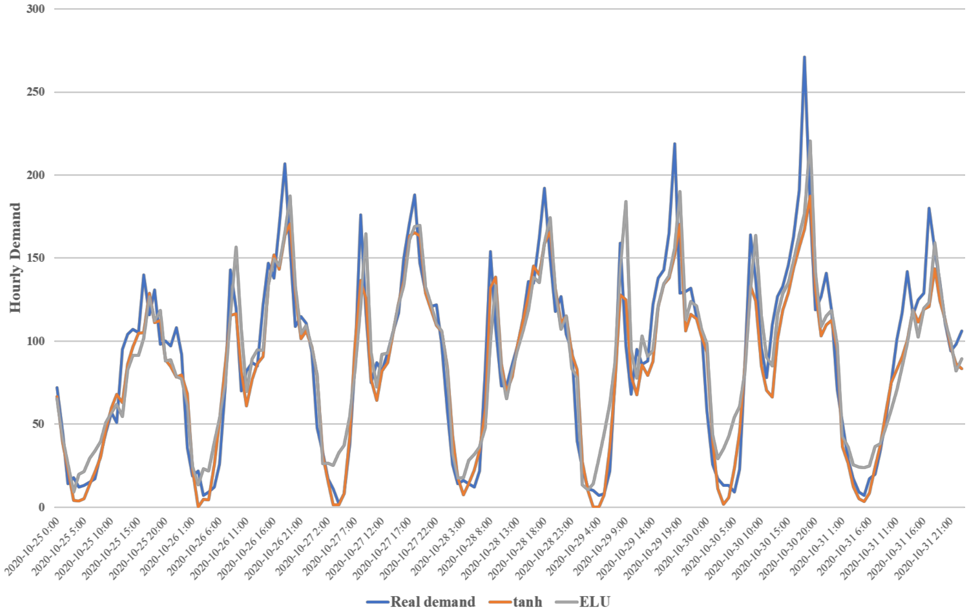
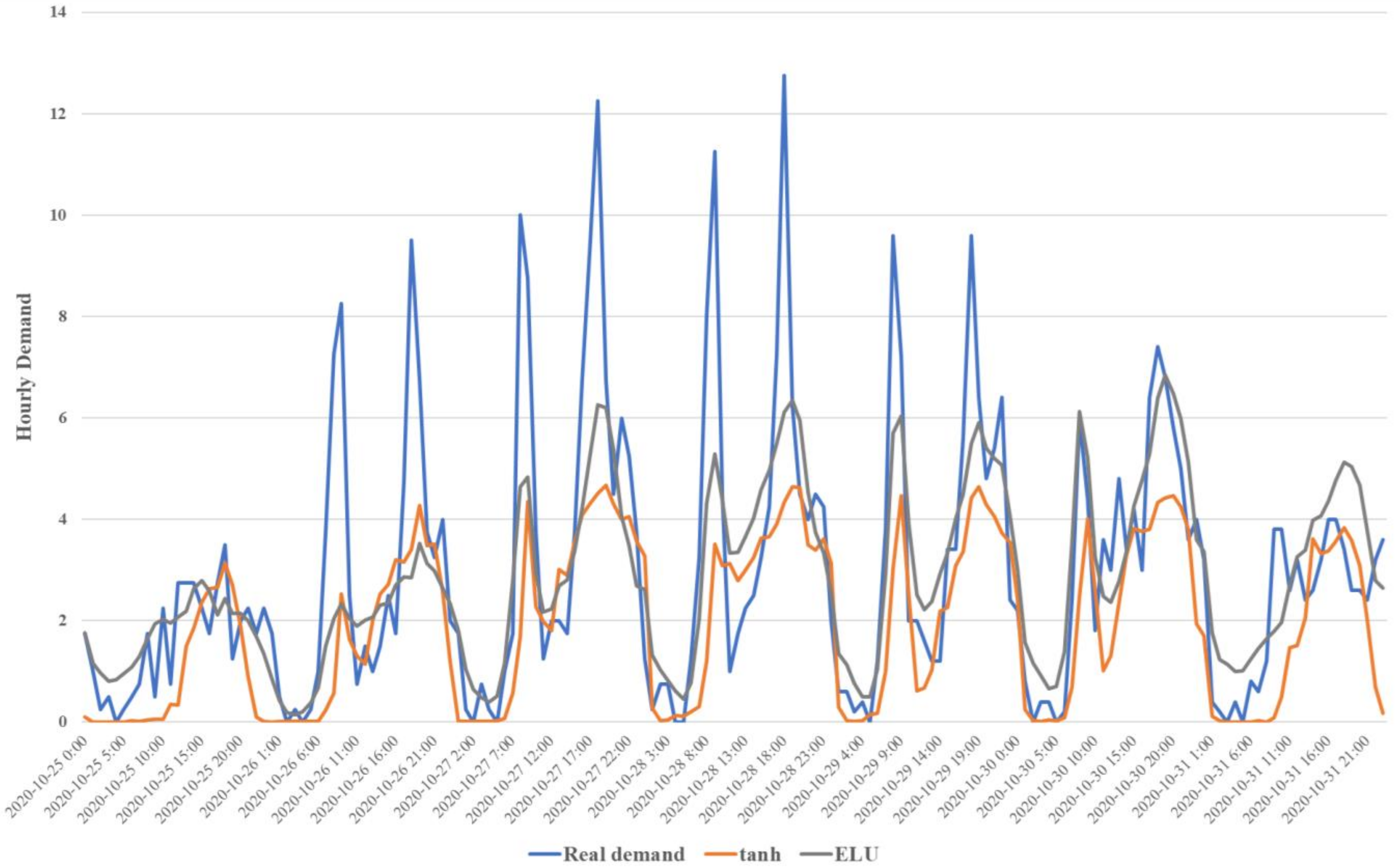
4.2. Prediction of Demand

We estimated the hourly demand for five communities and 1164 square grids. Existing studies have demonstrated that the LSTM used in this study has excellent predictive power when forecasting time series data [53,54,55,56]. LSTM and historical analysis (HA) were used to predict hourly demand. The LSTM presented all the results estimated by the four activation functions. The most suitable model was selected by evaluating the results on the basis of two indicators: mean squared error (MSE) and mean absolute error (MAE).

LSTM consists of several parameters. By adjusting the hidden state size and the number of hidden layers, which are the parameters of LSTM, an optimal model was developed for predicting hourly demand. Scenarios were set according to the hidden state and hidden layer, and the results of each scenario were compared. For the hidden state scenario, 2, 4, 6, and 8 were considered, and for the hidden layer scenario, 1, 2, 3, and 4 were considered.

Table 3. Performance of scenarios.

Evaluating Indicators	Hidden State Size (The Number of Hidden Layers Is 1)				Number of Hidden Layers (Hidden State Size Is 6)
	2	4	6	8	1	2	3	4
MSE	0.0134	0.0126	0.0065	0.0106	0.0065	0.0139	0.0139	0.0145
MAE	0.0716	0.0753	0.0608	0.0685	0.0608	0.0805	0.0749	0.0804

shows the results of each scenario. The model had the best predictive power when the size of the hidden state was 6. Additionally, the predictive power of the model decreased with increasing number of hidden layers. Therefore, the optimal model had a hidden state size of 6 and a number of hidden layers of 1.

Table 4. Performance of prediction model.

Activation Function		5 Partitions			1164 Square Grids
		MSE	MAE	Computing Time	MSE	MAE	Computing Time
LSTM	Sigmoid	0.0091	0.0739	109	0.0512	0.1707	5998
	Tanh	0.0065	0.0608	53	0.0507	0.1700	6390
	ReLU	0.0085	0.0677	50	0.0509	0.1710	6002
	ELU	0.0066	0.0604	78	0.0507	0.1702	5700
HA		0.0083	0.0618	-	0.1300	0.5440	-

shows the overall evaluation results of the optimal model. In the prediction results of five partitions, the lowest MSE of tanh among the activation functions of LSTM was found to be 0.0065. ELU also had an MSE of 0.0066, which was almost as low as tanh. In MAE, tanh and ELU were 0.0608 and 0.0604, respectively, so ELU was slightly more dominant. On the other hand, the MSE and MAE of HA were 0.0083 and 0.0618, respectively, indicating that its predictive power was lower than that of LSTM.

As a result of the prediction for 1164 square grids, the MSE and MAE of tanh were the lowest at 0.0507 and 0.1700, respectively. Compared with the prediction results of five partitions, the predictive power of 1164 square grids was determined to be lower. Additionally, comparing the computing time, the computing time for the five partitions took 50~109 s, while for 1164 square grids, it took 5700~6390 s.

The hourly demand of the orange community, which had the highest demand for use among the five communities, is shown in Figure 3. The hourly demand of tanh and ELU, which had excellent predictive power, was compared with the real demand. ELU was not good at predicting off-peak demand, but had excellent predictive power for peak-time demand. In contrast, tanh had better predictive power for off-peak than for peak-time demand. Therefore, it is necessary to use the appropriate activation function depending on the desired prediction time. Additionally, the hourly demand for the grid with the highest demand for use among the 1164 square grids is shown in Figure 4. Like the tanh of demand prediction by partition, demand prediction by grid was not good at predicting peak-time demand.

5. Conclusions

In this study, a prediction model was developed to predict the hourly demand for shared e-scooters using deep learning methods. The shared e-scooters’ trip data were collected for one month in Seocho and Gangnam, one of the CBDs in Seoul. Since shared e-scooters are a free-floating service without stations, the spatial unit was set to a 200 m square grid. The 1164 square grids in Seocho and Gangnam were grouped into five communities through the community structure method for analysis efficiency. The hourly demand prediction model was developed using LSTM, a deep learning method. Previous hourly demand, weather variables, and time variables of the community were used to predict hourly demand. As a result of the hourly demand prediction, the model that applied the ELU and tanh as the activation function well predicted peak time demand and off-peak demand, respectively.

Unlike previous studies that were limited to shared bicycle services, this study predicted the demand for shared e-scooters. This study is a case study that uses the methodologies (e.g., LSTM, community structure) of the previous studies to predict the demand for shared e-scooters. In this study, the predictive power of the analysis increased by additionally reflecting external variables (e.g., time variables, weather variables), and the computing time was shortened by clustering the analysis area; these were both aspects that had been suggested as limitations in previous studies [23,29,30]. We applied the community structure method to cluster the analysis area. On the basis of the findings of this study, we present a community structure method for the efficient analysis of the wide e-scooter service area.

Of course, this study also has some limitations. First of all, the temporal scope of this study was only one month. To improve the predictive power of the analysis, it is necessary to use data from over a longer period of time. In addition, it is necessary to reflect additional variables such as the built environment and the number of COVID-19 infections. The demand for shared e-scooters may be affected not only by time and weather, but also by regional characteristics and special events. In future research, we intend to develop a more sophisticated predictive model by supplementing these limitations and develop a relocation model based on it.

References

1. Clewlow, R.R. The Micro-mobility Revolution: The Introduction and Adoption of Electric Scooters in the United States. In Proceedings of the 98th Annual Meeting of the Transportation Research Board, Washington, DC, USA, 13–17 January 2019. [Google Scholar]
2. Liu, M.; Seeder, S.; Li, H. Analysis of E-scooter Trips and Their Temporal Usage Patterns. ITE J. 2019, 89, 44–49. [Google Scholar]
3. Shaheen, S.; Bell, C.; Cohen, A.; Yelchuru, B. Travel Behavior: Shared Mobility and Transportation Equity; Transportation Research Board: Washington, DC, USA, 2017. [Google Scholar]
4. McKenzie, G. Spatiotemporal Comparative Analysis of Scooter-share and Bike-share Usage Patterns in Washington, DC. J. Transp. Geogr. 2019, 78, 19–28. [Google Scholar] [CrossRef]
5. Dias, G.; Arsenio, E.; Ribeiro, P. The role of shared E-Scooter systems in urban sustainability and resilience during the COVID-19 mobility restrictions. Sustainability 2021, 13, 7084. [Google Scholar] [CrossRef]
6. Campisi, T.; Akgün-Tanbay, N.; Nahiduzzaman, M.; Dissanayake, D. Uptake of e-Scooters in Palermo, Italy: Do the Road Users Tend to Rent, Buy or Share? In International Conference on Computational Science and Its Applications; Springer: Cham, Switerland, 2021; pp. 669–682. [Google Scholar]
7. Kim, S.; Koack, M.; Choo, S.; Kim, S. Analyzing Spatial Usage Characteristics of Shared E-scooter: Focused on Spatial Autocorrelation Modeling. J. Korea Inst. Intell. Transp. Syst. 2021, 20, 54–69. [Google Scholar] [CrossRef]
8. Fang, K.; Agrawal, A.W.; Steele, J.; Hunter, J.J.; Hooper, A.M. Where Do Riders Park Dockless, Shared Electric Scooters? Findings from San Jose, California; Mineta Transportation Institute Publication: San Jose, CA, USA, 2018. [Google Scholar]
9. James, O.; Swiderski, J.I.; Hicks, J.; Teoman, D.; Buehler, R. Pedestrians and E-scooters: An Initial Look at E-scooter Parking and Perceptions by Riders and Non-riders. Sustainability 2019, 11, 5591. [Google Scholar] [CrossRef] [Green Version]
10. Zou, Z.; Younes, H.; Erdoğan, S.; Wu, J. Exploratory Analysis of Real-time E-scooter Trip Data in Washington, DC. Transp. Res. Rec. J. Transp. Res. Board 2020, 2674, 285–299. [Google Scholar] [CrossRef]
11. Raptopoulou, A.; Basbas, S.; Stamatiadis, N.; Nikiforiadis, A. A first look at e-scooter users. In Conference on Sustainable Urban Mobility; Springer: Cham, Switerland, 2020; pp. 882–891. [Google Scholar]
12. Bai, S.; Jiao, J. Dockless E-scooter Usage Patterns and Urban Built Environments: A Comparison Study of Austin, TX, and Minneapolis, MN. Travel Behav. Soc. 2020, 20, 264–272. [Google Scholar] [CrossRef]
13. Caspi, O.; Smart, M.J.; Noland, R.B. Spatial Associations of Dockless Shared E-scooter Usage. Transp. Res. Part D Transp. Environ. 2020, 86, 102396. [Google Scholar] [CrossRef]
14. Hosseinzadeh, A.; Algomaiah, M.; Kluger, R.; Li, Z. E-scooters and Sustainability: Investigating the Relationship Between the Density of E-scooter Trips and Characteristics of Sustainable Urban Development. Sustain. Cities Soc. 2021, 66, 102624. [Google Scholar] [CrossRef]
15. Lee, M.; Chow, J.Y.; Yoon, G.; Yueshuai He, B. Forecasting E-scooter Competition with Direct and Access Trips by Mode and Distance in New York City. arXiv 2019, arXiv:1908.08127. [Google Scholar]
16. Ham, S.; Cho, J.; Park, S.; Kim, D. Spatiotemporal Demand Prediction Model for E-Scooter Sharing Services with Latent Feature and Deep Learning. Transp. Res. Rec. J. Transp. Res. Board 2021, 2675, 34–43. [Google Scholar] [CrossRef]
17. Sikka, N.; Vila, C.; Stratton, M.; Ghassemi, M.; Pourmand, A. Sharing the Sidewalk: A Case of E-scooter Related Pedestrian Injury. Am. J. Emerg. Med. 2019, 37, 1807-e5. [Google Scholar] [CrossRef] [PubMed]
18. Trivedi, B.; Kesterke, M.J.; Bhattacharjee, R.; Weber, W.; Mynar, K.; Reddy, L.V. Craniofacial Injuries Seen with the Introduction of Bicycle-share Electric Scooters in an Urban Setting. J. Oral Maxillofac. Surg. 2019, 77, 2292–2297. [Google Scholar] [CrossRef] [PubMed] [Green Version]
19. Campisi, T.; Skoufas, A.; Kaltsidis, A.; Basbas, S. Gender Equality and E-Scooters: Mind the Gap! A Statistical Analysis of the Sicily Region, Italy. Soc. Sci. 2021, 10, 403. [Google Scholar] [CrossRef]
20. Chen, Y.W.; Cheng, C.Y.; Li, S.F.; Yu, C.H. Location Optimization for Multiple Types of Charging Stations for Electric Scooters. Appl. Soft Comput. 2018, 67, 519–528. [Google Scholar] [CrossRef]
21. Espinoza, W.; Howard, M.; Lane, J.; Van Hentenryck, P. Shared E-scooters: Business, Pleasure, or Transit? arXiv 2019, arXiv:1910.05807. [Google Scholar]
22. Turoń, K.; Kubik, A.; Chen, F. When, What and How to Teach about Electric Mobility? An Innovative Teaching Concept for All Stages of Education: Lessons from Poland. Energies 2021, 14, 6440. [Google Scholar] [CrossRef]
23. Chang, P.C.; Wu, J.L.; Xu, Y.; Zhang, M.; Lu, X.Y. Bike Sharing Demand Prediction using Artificial Immune System and Artificial Neural Network. Soft Comput. 2019, 23, 613–626. [Google Scholar] [CrossRef]
24. Xu, T.; Han, G.; Qi, X.; Du, J.; Lin, C.; Shu, L. A Hybrid Machine Learning Model for Demand Prediction of Edge-computing-based Bike-sharing System using Internet of Things. IEEE Internet Things J. 2020, 7, 7345–7356. [Google Scholar] [CrossRef]
25. Zhou, Y.; Wang, L.; Zhong, R.; Tan, Y. A Markov Chain Based Demand Prediction Model for Stations in Bike Sharing Systems. Math. Probl. Eng. 2018, 2018, 8028714. [Google Scholar] [CrossRef] [Green Version]
26. Yang, Y.; Heppenstall, A.; Turner, A.; Comber, A. using Graph Structural Information about Flows to Enhance Short-term Demand Prediction in Bike-sharing Systems. Comput. Environ. Urban Syst. 2020, 83, 101521. [Google Scholar] [CrossRef]
27. Pan, Y.; Zheng, R.C.; Zhang, J.; Yao, X. Predicting Bike Sharing Demand using Recurrent Neural Networks. Procedia Comput. Sci. 2019, 147, 562–566. [Google Scholar] [CrossRef]
28. Xu, C.; Ji, J.; Liu, P. The Station-free Sharing Bike Demand Forecasting with a Deep Learning Approach and Large-scale Datasets. Transp. Res. Part C Emerg. Technol. 2018, 95, 47–60. [Google Scholar] [CrossRef]
29. Ai, Y.; Li, Z.; Gan, M.; Zhang, Y.; Yu, D.; Chen, W.; Ju, Y. A Deep Learning Approach on Short-term Spatiotemporal Distribution Forecasting of Dockless Bike-sharing System. Neural Comput. Appl. 2019, 31, 1665–1677. [Google Scholar] [CrossRef]
30. Lin, L.; He, Z.; Peeta, S. Predicting Station-level Hourly Demand in a Large-scale Bike-sharing Network: A Graph Convolutional Neural Network Approach. Transp. Res. Part C Emerg. Technol. 2018, 97, 258–276. [Google Scholar] [CrossRef] [Green Version]
31. Zhang, H.; Wu, Y.; Tan, H.; Dong, H.; Ding, F.; Ran, B. Understanding and modeling urban mobility dynamics via disentangled representation learning. IEEE Trans. Intell. Transp. Syst. 2020, 1–11. [Google Scholar] [CrossRef]
32. Girvan, M.; Newman, M.E. Community Structure in Social and Biological Networks. Proc. Natl. Acad. Sci. USA 2002, 99, 7821–7826. [Google Scholar] [CrossRef] [Green Version]
33. Newman, M.E. Fast Algorithm for Detecting Community Structure in Networks. Phys. Rev. E 2004, 69, 066133. [Google Scholar] [CrossRef] [Green Version]
34. Blondel, V.D.; Guillaume, J.L.; Lambiotte, R.; Lefebvre, E. Fast Unfolding of Communities in Large Networks. J. Stat. Mech. Theory Exp. 2008, 2008, P10008. [Google Scholar] [CrossRef] [Green Version]
35. Zhang, J.; Meng, M.; Wang, D.Z.; Du, B. Allocation Strategies in a Dockless Bike Sharing System: A Community Structure-based Approach. Int. J. Sustain. Transp. 2022, 16, 95–104. [Google Scholar] [CrossRef]
36. Olah, C. Understanding Lstm Networks. 2015. Available online: http://colah.github.io/posts/2015-08-Understanding-LSTMs (accessed on 10 June 2021).
37. Huang, S.; Eichler, G.; Bar-Yam, Y.; Ingber, D.E. Cell Fates as High-dimensional Attractor States of a Complex Gene Regulatory Network. Phys. Rev. Lett. 2005, 94, 128701. [Google Scholar] [CrossRef] [PubMed] [Green Version]
38. Kaluza, P.; Kölzsch, A.; Gastner, M.T.; Blasius, B. The Complex Network of Global Cargo Ship Movements. J. R. Soc. Interface 2010, 7, 1093–1103. [Google Scholar] [CrossRef] [PubMed]
39. Rubinov, M.; Sporns, O. Complex Network Measures of Brain Connectivity: Uses and Interpretations. Neuroimage 2010, 52, 1059–1069. [Google Scholar] [CrossRef] [PubMed]
40. Sporns, O. The Human Connectome: A Complex Network. Ann. New York Acad. Sci. 2011, 1224, 109–125. [Google Scholar] [CrossRef] [PubMed]
41. Newman, M.E. Modularity and Community Structure in Networks. Proc. Natl. Acad. Sci. USA 2006, 103, 8577–8582. [Google Scholar] [CrossRef] [PubMed] [Green Version]
42. Clauset, A.; Newman, M.E.; Moore, C. Finding Community Structure in Very Large Networks. Phys. Rev. E 2004, 70, 066111. [Google Scholar] [CrossRef] [Green Version]
43. Ahn, Y.Y.; Bagrow, J.P.; Lehmann, S. Link Communities Reveal Multiscale Complexity in Networks. Nature 2010, 466, 761–764. [Google Scholar] [CrossRef] [Green Version]
44. Tealab, A. Time Series Forecasting using Artificial Neural Networks Methodologies: A Systematic Review. Future Comput. Inform. J. 2018, 3, 334–340. [Google Scholar] [CrossRef]
45. Sak, H.; Senior, A.; Beaufays, F. Long Short-term Memory Based Recurrent Neural Network Architectures for Large Vocabulary Speech Recognition. arXiv 2014, arXiv:1402.1128. [Google Scholar]
46. Graves, A.; Liwicki, M.; Fernández, S.; Bertolami, R.; Bunke, H.; Schmidhuber, J. A Novel Connectionist System for Unconstrained Handwriting Recognition. IEEE Trans. Pattern Anal. Mach. Intell. 2008, 31, 855–868. [Google Scholar] [CrossRef] [Green Version]
47. Hochreiter, S.; Schmidhuber, J. Long Short-term Memory. Neural Comput. 1997, 9, 1735–1780. [Google Scholar] [CrossRef] [PubMed]
48. Ma, X.; Tao, Z.; Wang, Y.; Yu, H.; Wang, Y. Long Short-term Memory Neural Network for Traffic Speed Prediction using Remote Microwave Sensor Data. Transp. Res. Part C Emerg. Technol. 2015, 54, 187–197. [Google Scholar] [CrossRef]
49. Ma, X.; Gildin, E.; Plaksina, T. Efficient Optimization Framework for Integrated Placement of Horizontal Wells and Hydraulic Fracture Stages in Unconventional Gas Reservoirs. J. Unconv. Oil Gas Resour. 2015, 9, 1–17. [Google Scholar] [CrossRef]
50. Gers, F.A.; Schraudolph, N.N.; Schmidhuber, J. Learning Precise Timing with LSTM Recurrent Networks. J. Mach. Learn. Res. 2002, 3, 115–143. [Google Scholar]
51. Zhao, Z.Z.; Chen, H.P.; Huang, Y.; Zhang, S.B.; Li, Z.H.; Feng, T.; Liu, J.K. Bioactive Polyketides and 8, 14-seco-ergosterol from Fruiting Bodies of the Ascomycete Daldinia Childi-ae. Phytochemistry 2017, 142, 68–75. [Google Scholar] [CrossRef]
52. Kingma, D.P.; Ba, J. Adam: A Method for Stochastic Optimization. arXiv 2014, arXiv:1412.6980. [Google Scholar]
53. Ese, N.; Esent, P. Long Short-Term Memory in Recurrent Neural Networks. Epfl 2001, 9, 1735–1780. [Google Scholar]
54. Shewalkar, A.; Nyavanandi, D.; Ludwig, S.A. Performance evaluation of deep neural networks applied to speech recognition: RNN, LSTM and GRU. J. Artif. Intell. Soft Comput. Res. 2019, 9, 235–245. [Google Scholar] [CrossRef] [Green Version]
55. Apaydin, H.; Feizi, H.; Sattari, M.T.; Colak, M.S.; Shamshirband, S.; Chau, K.W. Comparative analysis of recurrent neural network architectures for reservoir inflow forecasting. Water 2020, 12, 1500. [Google Scholar] [CrossRef]
56. Elsaraiti, M.; Merabet, A. A comparative analysis of the arima and lstm predictive models and their effectiveness for predicting wind speed. Energies 2021, 14, 6782. [Google Scholar] [CrossRef]
Figure 1. Unavailable areas, which are the red blocks on the app execution screen (left), and spatial area based on Kakao map in Seocho and Gangnam (right).
Sustainability 14 02564 g001
Figure 2. Modularity of partition results (left) and the result of service cluster based on Kakao map (right).
Sustainability 14 02564 g002
Figure 3. Hourly demand and the prediction results thereof in community orange.
Sustainability 14 02564 g003
Figure 4. Hourly demand and prediction results thereof in the highest demand grid.
Sustainability 14 02564 g004