Improving Sustainable Vegetation Indices Processing on Low-Cost Architectures

Abstract

The development of embedded systems in sustainable precision agriculture has provided an important benefit in terms of processing time and accuracy of results, which has influenced the revolution in this field of research. This paper presents a study on vegetation monitoring algorithms based on Normalized Green-Red Difference Index (NGRDI) and Visible Atmospherically Resistant Index (VARI) in agricultural areas using embedded systems. These algorithms include processing and pre-processing to increase the accuracy of sustainability monitoring. The proposed algorithm was evaluated on a real database in the Souss Massa region in Morocco. The collection of data was based on unmanned aerial vehicles images hand data using four different agricultural products. The results in terms of processing time have been implemented on several architectures: Desktop, Odroid XU4, Jetson Nano, and Raspberry. However, this paper introduces a thorough study of the Hardware/Software Co-Design approach to choose the most suitable system for our proposed algorithm that responds to the different temporal and architectural constraints. The evaluation proved that we could process 311 frames/s in the case of low resolution, which gives real-time processing for agricultural field monitoring applications. The evaluation of the proposed algorithm on several architectures has shown that the low-cost XU4 card gives the best results in terms of processing time, power consumption, and computation flexibility.

1. Introduction

Precision agriculture can be considered a research field that focuses on using different tools to increase agricultural fields’ productivity [1]. Generally, it is based on various sensors depending on the field of application [2,3]. Among these sensors, we can find different types of cameras, from Red, Green, Blue (RGB) to hyperspectral and multispectral cameras. All these tools have a common goal based on increasing yield and production improvement [4]. The algorithmic side in precision agriculture is rich and depends on the nature of the application chosen. These applications aim to solve different problems encountered in traditional agriculture. For example, weeds, various plant diseases, as well as monitoring vegetation and vital visual signs using different indices [5,6,7,8]. These applications require a feasibility study in real scenarios to validate the different approaches proposed in the literature. As a solution, the use of embedded systems can help not only the validation but also the improvement of the different methods. The implementation of these methods requires an algorithmic and architectural study in order to propose optimal implementations that increase the reliability of calculation as well as reduce the processing time in applications that require a precise time. Besides processing time and reliability, we can also find the calculation accuracy in the different data collection tools [9]. For example, robots and unmanned aerial vehicles are equipped with various tools that help the autonomous mobility of these robots. The accuracy of movement can be solved using GPS sensors or localization and mapping algorithms. But the problem here is that this autonomous movement of robots or Unmanned Arial Vehicle (UAVs) can create problems such as camera blur as well as memory saturation, which can influence the quality of the results obtained.

In fact, several approaches have been developed based on embedded systems, but they remain limited in real-time constraints as well as in time and complexity. For example, J. Rodríguez et al., 2021 proposed a system for monitoring potato fields. The work was based on a Tarot 680PRO hexacopter UAV and a MicaSense RedEdge multispectral camera. The authors used two types of data A and B; the results showed high accuracy in field A while field B had low accuracy [10]. For the monitoring of agricultural fields, we can also find the work of [11], which was based on a drone and a multispectral camera to monitor agricultural fields. Similarly, for the detection of weeds, A. Wang et al., 2020 used deep learning approaches to detect weeds. The study presented a detection accuracy about 96.12% [12]. The work of S. Abouzahir et al., 2021 detects weeds on several types of crops based on an embedded platform with an accuracy that varies between 71.2% and 97.7% [13]. In the case of counting plants, we can also find S. Tu et al., 2020 who proposed a fruit counting approach based on depth calculation to increase the counting accuracy. The work showed a counting accuracy and an F1 score that reaches up to 0.9 [14]. All these approaches and systems proposed give us an idea of the different algorithms and embedded architecture proposed in this sense. This reflects the massive evolution of precision agriculture. However, the problem of these algorithms is the evaluation in real cases where time influences the accuracy of the results. This pushes us to investigate further the study of how we can embed these algorithms in low-cost architecture and energy consumption to guarantee an autonomy of treatment without the intervention of farmers. In addition, these algorithms and their implementation require a preprocessing that includes the detection of blur and its elimination that directly influences the accuracy and reliability of the results. Another critical factor when we talk about applications based on soil robots and UAVs is the memory saturation that requires data compression after their processing, which we will address in this study.

In our work, we propose a system divided into three parts. The first part focuses on the measurement of blur and then the elimination of this blur. In this context, we have used a hybrid algorithm that combines blur measurement and filtering to ensure images without motion. This blur removal algorithm uses blur measurement before removal compared to the other technique proposed in the literature, which is only based on blur suppression without measurement [15]. The second part calculates the most general indices based on RGB images. These indices are NGRDI and VARI; choosing these indices is due to the high sensitivity to agricultural land cover [16]. Moreover, they are easy to interpret compared to other indices, which are strongly related to our study. The third part of the work focused on studying the memory saturation problem. We have added a compression algorithm to eliminate this significant problem as a solution. These three parts combined on a single algorithm that processes agricultural fields’ images in real-time. Our novelty and contribution are as follows:

(1)

The proposition of a new algorithm based on various techniques for compression, blur detection, and RGB indices processing such as NGRDI and VARI.

(2)

The evaluation of the algorithm was based on our original database using a Phantom DJI pro 4 drone in different agricultural areas.

(3)

The study of the temporal constraints was proposed based on the Hardware/Software Co-Design approach.

(4)

A hardware acceleration was developed on several low-cost embedded architectures in order to respect the architectural and temporal constraints.

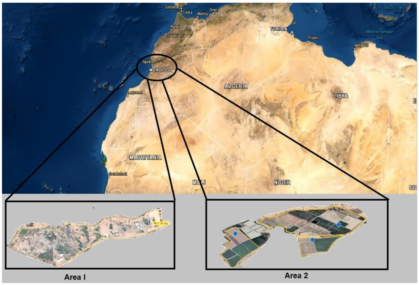
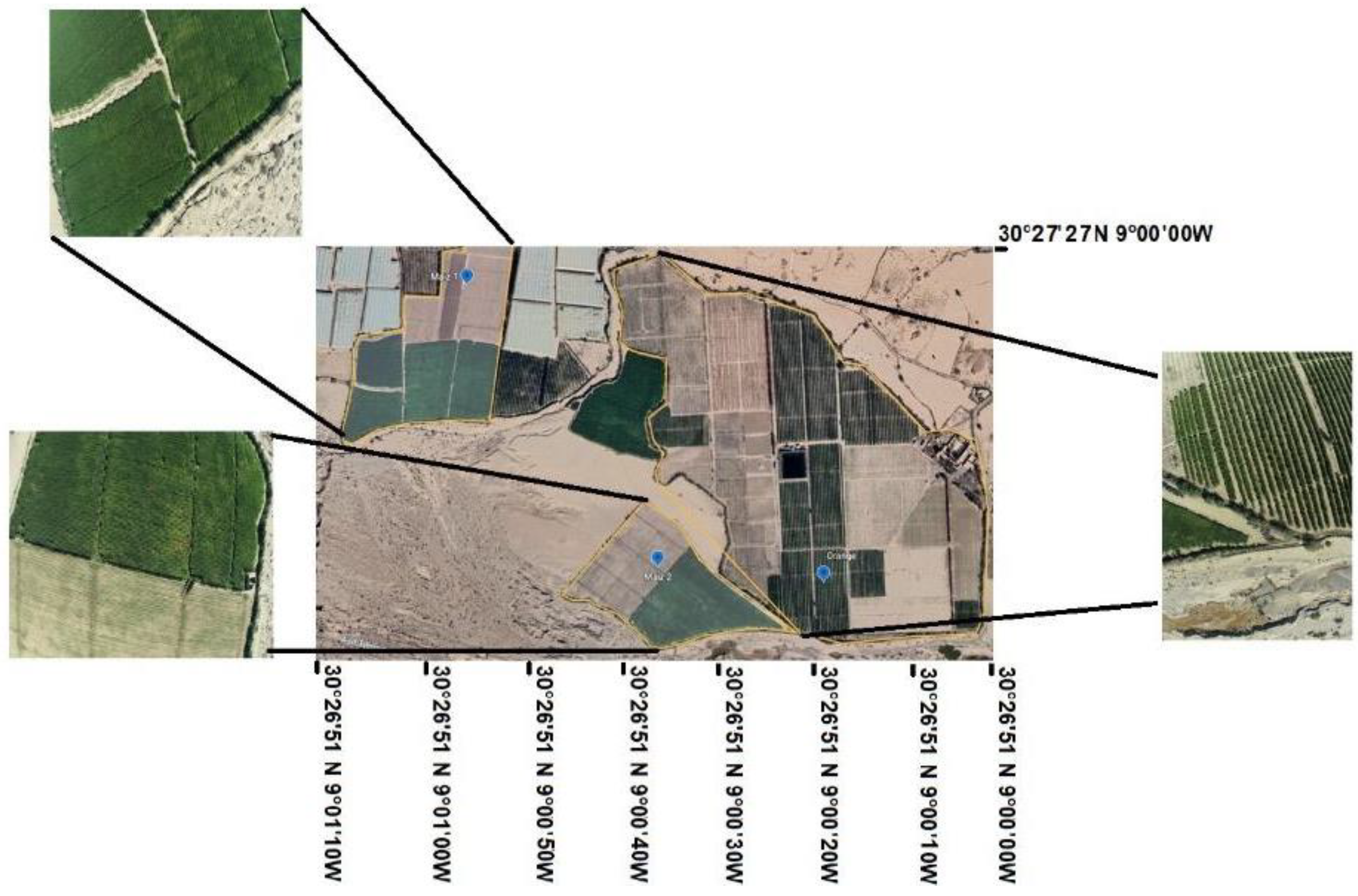
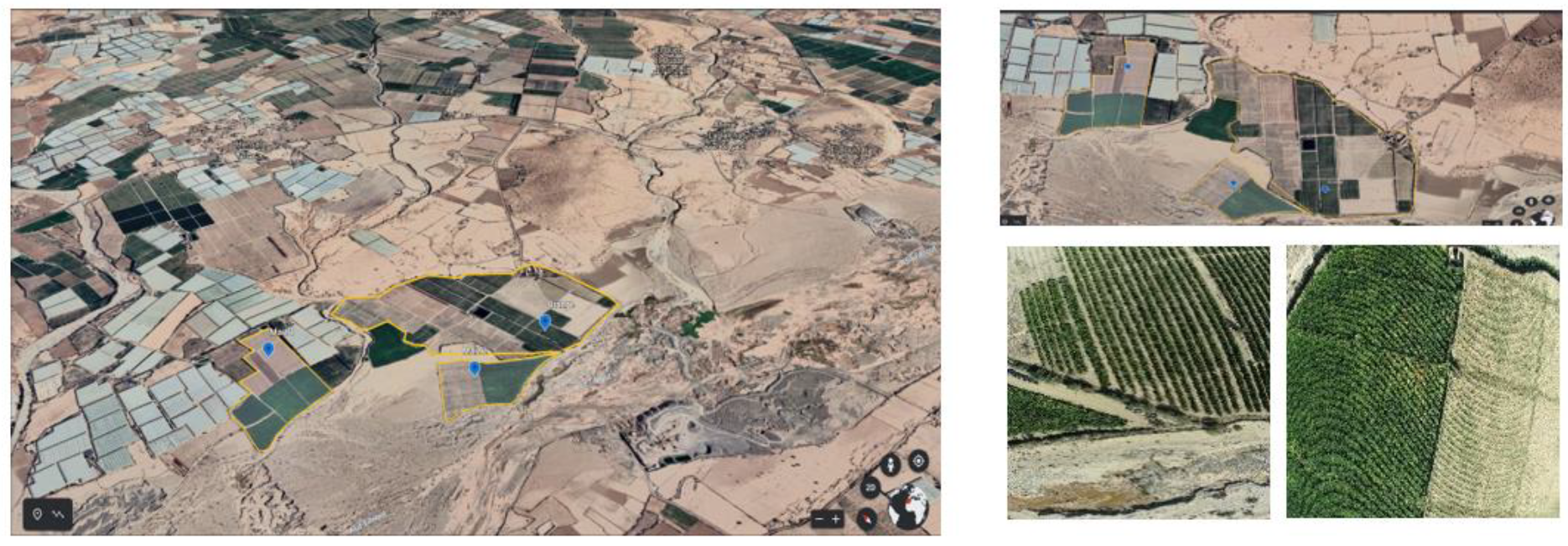
Our algorithm has been evaluated on several embedded systems such as XU4, Jetson Nano, and Raspberry. The objective of these implementations is to study the adequacy between the hardware and the software. The results showed that the XU4 card remains the best choice for our application, thanks to its low consumption and cost, as well as the solid, parallel computation. The tools used in this evaluation are based on C/C++, OpenMP, and OpenCL. The C/C++ language has been used to validate the algorithm proposed in the chosen system and OpenMP to exploit the parallelism in the selected card. For OpenCL, we used it to exploit the Graphics Processing Unit (GPU) part of our card for acceleration in order to minimize the processing time. The proposed algorithm has a complexity of O = K × (i × j) Log2 (i × j), where K is the number of data used and i × j is the image size. This study’s data were based on the Souss Massa region’s agriculture in the south of Morocco, which is considered one of the most productive regions of agriculture in Morocco. Our database was collected using UAV type DJI and RGB cameras for the fields of maize and orange, as well as a hand database for parsley and mint.

Our paper is summarized as follows: the first part focuses on the different recent works and an overview of the RGB index used in agriculture. The second part describes our methodology based on the algorithmic study and the agricultural fields that have been used. The third part is based on the proposed implementation and the software–hardware results obtained from the embedded systems used. Then, we have the real results obtained from the selected agricultural fields. Finally, we finish with a conclusion and future work.

2. Background and Related Work

Monitoring in agricultural fields helps a significant part of farmers to construct an idea about the different plants. This monitoring needs a special system able to extract useful information in the agricultural fields. Among the most relevant information in the crop coverage, we find the vegetation indexes. These indexes are based on algebraic equations that use as an argument the special bands of the cameras. Usually, the bands used vary between the different indices that will be used later. Vegetation in plants is based on an absorption and reflection process of the red, green, blue, shortwave, and near-infrared bands. Each reflection or absorption of these bands indicates different indices. For example, to calculate the vegetation and water index, it is necessary to use the R, G, B, and Near InfraRed (NIR) bands. On the other hand, the humidity index is based on the Short Wave Near-InfraRed (SWIR) and R waves. Data collection is done using several tools; the choice depends on the specific application. We can also find indices based on the R, G, and B bands only; these indices have proved a reliable precision in monitoring agricultural fields.

Table 1. RGB vegetation index.

Index	Algebraic Equation	Purpose Utility	References
NGRVI	$\frac{B_{Green}-B_{Red}}{B_{Green}+B_{Red}}$	Normalized Green-Red Vegetation Index (NGRVI) used to identify the vegetal biomass in plants	E.R. Hunt et al., 2005 [17]
MGRVI	$\frac{{(B_{Green})}^2-{(B_{Red})}^2}{{(B_{Green})}^2+{(B_{Red})}^2}$	Modified Green-Red Vegetation Index (MGRVI) dedicated to measure the absorption of chlorophyll	J. Bendig et al., 2015 [18]
RGBVI	$\frac{{(B_{Green})}^2-{(B_{Red}\times B_{Blue})}^2}{{(B_{Green})}^2+{(B_{Red}\times B_{Blue})}^2}$	Red-Green-Blue Vegetation Index (RGBVI) dedicated to measure the absorption of chlorophyll	J. Bendig et al., 2015 [18]
VARI	$\frac{B_{Green}-B_{Red}}{B_{Green}+B_{Red}-B_{Blue}}$	Visible Atmospherically Resistant Index dedicated to vegetation rate calculation	A.A. Gitelson et al., 2002 [19]

shows the different indexes based on the three RGB bands.

Table 1 shows the most common vegetation indices used in precision agriculture; these indices are easy to calculate using RGB cameras. However, the Normalized Difference Vegetation Index (NDVI) aims to extract the vegetation amount from various plants and requires a multispectral camera, which is expensive compared to RGB cameras. A.A. Gitelson et al. showed that the VARI presented an error of <10% vegetation fraction [19]. This shows the robustness of this index for vegetation estimation. The evaluation of the index was on a region near the city of Beer-Sheva, Israel. The authors in [18] used a UAV to calculate these indexes with an acquisition frequency of two frames/s [18]. We also find the work of P. Ranđelović et al., 2020, which was based on RGB indexes in order to predict plant density [20].

The scientific literature presents various tools, but the most well-known and effective ones are the sole robot, the satellite, the UAVs, and the hand data. We can also find several sensors such as RGB, multispectral, and hyperspectral cameras. All these tools and sensors have a common goal based on monitoring and tracking the agricultural fields’ plantations. Nowadays, several works have been elaborated in this context, aiming to improve the quality of monitoring and the reliability of the results. D. Shadrin et al., 2019 propose an embedded system based on GPU that does plant growth analysis via artificial intelligence. They used an algorithm based on Long Short-Term Memory (LSTM); the evaluation of this algorithm was on a Desktop and a Raspberry Pi 3B card. The embedded tool used in this study is the GPU card, but the weak point here is the limitation of the Raspberry card at the level of computation in the GPU; also, these cards do not support the Compute Unified Device Architecture (CUDA) tool that accelerates processing in the GPU card. However, this work’s results have been detailed and are rich in information either at the level of execution time or the low energy consumption [21]. Another work has been proposed to ensure robots’ autonomous movement to perform tasks such as weed detection, plant counting, or vegetation monitoring. The result was based on applying localization and mapping algorithms in agricultural fields using different Simultaneous Localization and Mapping (SLAM) algorithms. However, the work was evaluated on a laptop, and no embedded study has been made. This pushes us to conclude that the evaluation of these types of algorithms in conventional machines does not apply the implementation in low-cost embedded systems to ensure the optimal movement of the robot in agricultural fields. However, the work has shown the usefulness of the localization and mapping algorithms that were developed just for the automotive field, which shows that these algorithms can also be helpful in the agricultural area [22]. X.P. Burgos-Artizzu, et al., 2011 proposed two subsystems for agricultural field monitoring and weed detection. The first system is dedicated to trajectory identification and the second one to weed detection. The algorithm was evaluated on a desktop with eight frames/s processing based on C++ language; the results showed an accuracy of 90% for weed detection [23].

Table 2. Vegetation indexes-based application and tools.

Work	RGB Index Used	Application	Data Tools	Camera Type	References
J. Bendig et al., 2015	NGRVI, RGBVI	Biomass monitoring	UAV	RGB	[18]
P. Ranđelović et al., 2020	VIs (Vegetation indices)	Plant density	UAV	RGB	[20]
M.d.J. Marcial-Pablo et al., 2019	ExG, VIg	Estimation of vegetation cover	UAV	RGB, and Multispectral	[24]
K.C. Sumesh et al., 2020	ExG, GRVI, SI	Estimate of production in sugarcane fields	UAV	RGB	[25]
P. Ranđelović et al., 2020	VIs	Calculation of soybean plant density	UAV	RGB	[20]
T. De Swaef et al., 2021	VIs	Evaluation of drought in forage grasses	UAV	RGB, and Thermal	[26]
N. Chebrolu et al., 2017	--	Sugar beet classification	Sol robot	RGB-D	[27]
C. Potena et al., 2019	ExG	Agricultural field monitoring	UGV and UAV	RGB-D and RGB	[28]
X. Zhou et al., 2021	VIs	Vineyards monitoring	UAV and satellite	UAV and Sentinel-2	[29]

presents a synthesis of the different works on agricultural field monitoring.

All these applications have been based on the monitoring of indices. These RGB indices are an alternative to the index based on multispectral cameras. This alternative allows us to monitor agricultural fields based on low-cost systems such as RGB cameras. The scientific development of embedded systems has enabled us to have a flexibility of choice, generally characterized by the use of low power, cost, and performance architecture, especially if we consider autonomous applications that do not require intervention. For this reason, if we want to develop this kind of system, we will have to consider the algorithmic, architecture, and energy consumption constraints, keeping the reliability and precision of the results [24]. The use of embedded systems in agriculture will help us to achieve complicated tasks as fast as possible. Generally, we find a variety of systems; these systems are divided into two parts, either homogeneous, which is based on CPU, FPGA, and DSP, or heterogeneous, which combines CPU and CPU/GPU/FPGA/DSP; their primary role is the acceleration of algorithms based on high-level language. Usually, C/C++ is dedicated to homogeneous systems like CPU and DSP. For the construction of dedicated architecture, we can find the use of FPGA, which is characterized by low energy consumption. Still, its weak point is the coding complexity in this type of architecture. The C/C++ language is generally limited in the context where we want to speed up the processing [30,31,32]. For this reason, the OpenMP directive remains an excellent solution to accelerate the code in C/C++.

On the other hand, CUDA and OpenCL offer a high-performance acceleration in heterogeneous systems type CPU-GPU for CUDA and CPU-GPU/FPGA/DSP for OpenCL. Despite its huge advantage, CUDA remains limited in heterogeneous systems due to its use only for Nvidia architecture, which encourages the use of OpenCL that gives flexibility in different architectures. For this reason, we have chosen to use OpenMP and OpenCL. The use of these languages as well as heterogeneous systems is still very limited in precision agriculture, as most of the works are based on software and workstations, which restrict the use of autonomous systems in real scenarios.

The non-use of embedded systems makes the processing offline, and this processing does not take into consideration a variety of problems that it can be confronted with. Among these problems, we can find the blur generated by the type of cameras or movement of tools used for data collection, either robots or UAVs. This blur can affect the reliability of the results, which does not respect the constraints of an autonomous embedded system [33]. Moreover, a very critical parameter influencing the data collection is memory saturation [34].

3. Methodologies and Area Study

In this part, we will focus on our field of study as well as the methodology for the evaluation of our contribution.

3.1. Area Study 1

Agriculture in the Souss Massa region in Morocco is very interesting. It occupies an important percentage of the national agriculture. The choice of this region in our study is due to the variety of agricultural products. Our field of study is separated into four agricultural products, namely maize, oranges, parsley, and mint. These four products are separated into two agricultural areas. Figure 1 shows the fields used in this study.

3.1.1. Area I

The first area contains two types of products: mint and parsley, and it is located in the Souss Massa region in the south of Morocco. Mint is a highly effective plant that can grow up to 80 cm high. It belongs to the family of Lamiaceae. The most used compounds are menthol (between 35% and 55%) and menthone (10% to 40%). Mint has several types; in our case, we used the green mint. Just like parsley, it is a real mine of nutritional qualities. The collection of the images was done in February 2021 for mint and parsley. The agricultural area has a surface of 821 ha, which varies between mint and parsley. The choice of these two agricultural products is due to the great demand for them in this region as well as the great surface reserved for this type of product. These images were based on a hand database collection, which presents a low-cost technique of image collection. The database contains more than 100 images of different positions in the agricultural area. Due to the large surface of the farming fields in the mentioned products, we have chosen two small surfaces to make our study. The first field is mint, which contains a total surface of 1.27 ha, and the second one is parsley, with 3.08 ha calculated with GPS, which implies 12,700 m² for the mint and 30,800 m² for the parsley. The two selected fields are located between Lat 30°22′01″ N, Long 9°29′32″ W, and Lat 30°22′01″ N, Long 9°29′24″ W, for ↔, as well as between Lat 30°22′05″ N, Long 9°29′24″ W and Lat 30°22′15″ N, Long 9°29′26″ W for ↕. Figure 2 shows the location of selected fields.

For the mint field, it is separated into small squares of 2 m × 2 m throughout the area, which can give in the high season up to seven packets for each square. For the parsley, we have a rectangle of 3 m × 1.5 m with ten boxes approximately, according to the experience of the farmers in the region. Figure 3 shows images of the database of the first area. Part 1 in Figure 3 shows the mint, and part 2, the parsley. The database was collected using a Samsung SM-J8 10F camera with a resolution of 5256 × 3790 for the first database, which contains the two agricultural products mint and parsley.

3.1.2. Area II

The second area of study contains two agricultural products: oranges and maize. These areas are also located in the Souss Massa region near Agadir city. The choice of these two types of products is due to the large field reserved for these types of products in this region, which encourages the study of oranges and maize. This region of southern Morocco contains large farms reaching up to 40,000 ha for citrus, representing a percentage of 30%; for maize, we find two types: sweet corn and forage corn. The sweet corn can reach up to (0.7–0.9 m) × 0.3 m. The population density recommended for forage maize ranges from 6 to 10 plants per m², corresponding to a seeding density of approximately 20 to 30 kg/ha. For the early varieties, the density varies from 8 to 10 plants/m², and in the late varieties, the density varies between six and seven plants per m². The distance between the rows is 60 to 80 cm, with a space of 13 to 21 cm between each plant. Our study has chosen three fields, two for the maize and one for the oranges. The field of the oranges has a surface of 51.5 ha with a perimeter of 3.3 km, and for the first field of maize, 13.6 ha with a perimeter of 1. 82 km, and for the second field of maize, we have an area of 9.34 ha with a perimeter of 1.45 km. The selected fields are located between 30°26′51″ N, Long 9°01′10″ W and 30°26′51″ N, Long 9°00′00″ W for ↔, and from 30°26′51″ N, Long 9°00′00″ W until 30°27′27″ N, Long 9°00′00″ W for ↕. Figure 4 shows the location of the second study area.

The second database was collected by an unmanned aerial vehicle based on an RGB camera. The type of camera is DJI model FC6310R with a resolution of 5472 × 3648. The type of UAV used is DJI Phantom Pro 4. Figure 5 shows the two fields of maize and orange.

Therefore, we can conclude that we have two databases, one collected by hand and the other using unmanned aerial vehicles. We have four agricultural products, two for the first database and two for the second. Figure 6 and

Table 3. Database specification.

Crop Types	Surface	Tools	Resolution	Location	Camera Specification	Altitude
Maize	S1 = 13.6 ha, S2 = 9.34 ha	UAV (DJI Phantom Pro4)	5472 × 3648	East of the Souss Massa region, Morocco	Focal: F/5.6, Focal distance: 9 mm	356 m
Orange	S = 51.5 ha	UAV (DJI Phantom Pro4)	5472 × 3648	East of the Souss Massa region, Morocco	Focal: F/5.6, Focal distance: 9 mm	356 m
Mint	S = 1.27 ha	Hand	5256 × 3790	Agadir (the Souss Massa region), Morocco	Focal: F/1.7, Focal distance: 4 mm	__
Parsley	S = 3.08 ha	Hand	5256 × 3790	Agadir (the Souss Massa region), Morocco	Focal: F/1.7, Focal distance: 4 mm	__

show the characteristics of each database.

Table 3 shows the different specifications of the collected databases, i.e., the tools used, the resolution of the images, the type of crop, and the altitude in the case of UAVs, as well as the surface of each field, where S1 is the surface of Maize 1 fields and S2 the surface of Maize 2 fields.

3.2. Methodologies

Our methodology focuses on four steps to study a real scenario of a plant index monitoring system. Generally, we have the acquisition step, then the measurement and blur detection, the index calculation, and the image compression to reduce images size for storage.

3.2.1. Image Acquisition

The acquisition of the images was based on two low-cost RGB cameras in order to build the database that will be evaluated in the following paper. The collected images were divided into two databases: one collected by hand and the other with a UAV type DJI phantom Pro4 in two different areas. The UAV used for the acquisition has a Dual Frequency Control Signal of 2.4 and 5.8 Ghz, with a 7 km range, with a flight time of 30 min. The drone’s weight is 1388 g, and it integrates a GPS/GLONASS. The precision of displacement of this tool is about ±0.1 m for the vertical position and ±0.3 m for the horizontal position. Each image collected by the UAV integrates the different information needed to show the type of camera used and the image’s different characteristics (i.e., focal length, exposure time, and other). The precise localization is based on the GPS coordinates of each image. This will provide a database with the coordinates of each image collected. Then, we also find the altitude of the UAV in the time it collected the image.

3.2.2. Blur Detection

Blur detection and elimination are very important steps to avoid images containing a high amount of noise, such as blur. In a real case, blur is among the most encountered problems in image acquisition; this blur is generated due to the source movement that collects the data, between the camera and the scene during the exposure time. For example, in the case of a drone, this blur can be created when we have a movement caused by wind. For the ground robots, we can also find the blur caused by the movement of robots in agricultural fields. For this reason, the blur measurement is very important in this case. Generally, blur elimination is based on several techniques, but the most used that we find is the filter of Wiener, Discrete Fourier Transform (DFT) and Lucy-Richardson (LR) [35,36,37]. Generally, blur elimination techniques aim to extract the image and eliminate the blur kernel. The representation of an image with blur is shown in Equation (1).

B_L = O_{_i} ⨂ K__b + ß

(1)

where B_L is the blurred image, K__b is the blur kernel, O__i unblurred image, and ß is overload noise in the image. Equation (1) was used based on images without blur to add blur, as shown in the equation. This technique allowed us to add the blur to some images in our data to test the algorithm’s different functionality. If there is a blurred image, then it will filter it; if not, then it will move directly to the processing. The technique chosen in our case is based on the Discrete Fourier Transform (DFT), thanks to its low complexity compared with other iterative methods such as LR and Wiener. The other techniques are based on the repetition approach to eliminate blur, which can create a problem at the level of temporal constraint. In our case, low-time processing is very important to avoid a processing latency, and the high complexity will also influence our study. For this reason, we chose the DFT technique based on low complexity conventional products. Equations (2)–(4) describe the Discrete Fourier Transform and the convolution product [38].

$$\begin{gathered} {\mathrm{C}}_{\mathrm{p}} \left(\begin{array}{c}\left(\mathrm{i}=0,\mathrm{j}=0\right)\cdots \left(\mathrm{i}=0,\mathrm{j}={\mathrm{C}}_1\right)\\ ⋮ ⋮ ⋮ \\ \left(i={\mathrm{L}}_1,j=0\right) \cdots \left(i={\mathrm{L}}_1,j={\mathrm{C}}_1\right) \end{array}\right) = {\mathrm{I}}_{\mathrm{image}} \left(\begin{array}{c}\left(\mathrm{i}=0,\mathrm{j}=0\right)\cdots \left(\mathrm{i}=0,\mathrm{j}={\mathrm{C}}_2\right)\\ ⋮ ⋮ ⋮ \\ \left(i={\mathrm{L}}_2,j=0\right) \cdots \left(i={\mathrm{L}}_2,j={\mathrm{C}}_2\right) \end{array}\right) \\ ⨂ \mathrm{F} \left(\begin{array}{c}\left(\mathrm{i}=0,\mathrm{j}=0\right)\cdots \left(\mathrm{i}=0,\mathrm{j}=\mathrm{C}\right)\\ ⋮ ⋮ ⋮ \\ \left(i=L,j=0\right) \cdots \left(i=L,j=C\right) \end{array}\right) \end{gathered}$$

(2)

which implies (2)

$${\mathrm{I}}_{\mathrm{image}}\left(\mathrm{i},\mathrm{j}\right)⨂\mathrm{F}\left(\mathrm{i},\mathrm{j}\right)={\sum }_{\mathrm{m}=0}^{\mathrm{L}-1} {\sum }_{\mathrm{n}=0}^{\mathrm{C}-1}{ \mathrm{I}}_{\mathrm{image}}\left(\mathrm{L},\mathrm{C}\right) \mathrm{F}\left(\mathrm{i}-\mathrm{m},\mathrm{j}-\mathrm{n}\right)$$

For the convolution product, we have C_p(i,j) the convolution results, I_image (i,j) the input image, and F(i,j) the convolution object [36]. Moreover, we have 0 ≤ i, m ≤ L-1; and 0 ≤ j, n ≤ C-1, with L × C the dimensions of F(i,j) and L₁ × C₁ for Cp and L₂ × C₂ for I_image.

Then, the Discrete Fourier Transform (DFT) of image I_image (i,j) [38]:

$$\mathrm{F}\left(\mathrm{x},\mathrm{y}\right)={\displaystyle \sum }_{\mathrm{i}=0}^{{\mathrm{L}}_2-1}{\displaystyle \sum }_{\mathrm{j}=0}^{{\mathrm{C}}_2-1}{ \mathrm{I}}_{\mathrm{image}}\left(\mathrm{i},\mathrm{j}\right){\mathrm{e}}^{-\mathrm{j}2\mathsf{\pi }\left(\frac{\mathrm{xi}}{{\mathrm{L}}_2}+\frac{\mathrm{yj}}{{\mathrm{C}}_2}\right)}$$

(3)

where I_image(i,j) is the input image with size L₂ × C₂, and the discrete variables x = 0,1,2,3….. → L₂-1 and y = 0,1,2,3….. → C₂-1. For the reverse or inverse DFT we have:

$${\mathrm{I}}_{\mathrm{image}}\left(\mathrm{i},\mathrm{j}\right)={\displaystyle \sum }_{\mathrm{i}=0}^{{\mathrm{L}}_2-1}{\displaystyle \sum }_{\mathrm{j}=0}^{{\mathrm{C}}_2-1} \mathrm{F}\left(\mathrm{x},\mathrm{y}\right){\mathrm{e}}^{\mathrm{j}2\mathsf{\pi }\left(\frac{\mathrm{xi}}{{\mathrm{L}}_2}+\frac{\mathrm{yj}}{{\mathrm{C}}_2}\right)}$$

(4)

Equation (2) is based on the convolution product between the convolution object in our case, a matrix F(i,j), and the input image I_image, which is also a matrix of pixels that have i,j as dimension. Similarly, Equations (3) and (4) present Discrete Fourier Transform (DTF) and Inverse Discrete Fourier Transform (iDFT), based on the input image I_image. We also have the results of the Fourier Transform that will be stored in an output image F(x,y). These two equations have been used in our work for the blur elimination part.

Table 4. Variable description of the equations used.

Equation	Variables	Description
2	CP	Convolution results
	Iimage	Input image
	F	Convolution object
	L × C	Dimensions of F
	L1 × C1	Dimensions of CP
3,4	Iimage	Input image
	L2 × C2	Dimensions of Iimage
	x,y	Discrete variables, vary between 0 and L2-1 for x and 0 to C2-1 for y
5,6	N	Number of blocks for Discrete Cosine Transform (DCT).
	D	Discrete Cosine Transform
	a,b	Variables of Discrete Cosine Transform range from 0 to N-1

shows the description of the variables used in the different equations.

The blur measurement is very important for good image filtering, but we also used this option to reduce processing time in our hybrid algorithm. If we have a significant amount of blur calculated from mask of the Laplacian, then it is necessary to apply blur elimination. Otherwise, it will pass directly to the calculation of indices. The blur elimination algorithm is based on three mathematical approaches: the convolution product, the Discrete Fourier Transform (DFT), iDFT, and Laplacian (LPA). The first step aims to measure the blur and then apply a thresholding operation to determine if the image contains blur or not. This test operation will help us pass the blur elimination procedure if the captured image does not have blur, minimizing the overall processing time. If the image contains blur, it will apply the Discrete Fourier Transform and the convolution product between the measured kernel gaussian DFT and the image DFT to recover the unblurred image based on the Inverse Discrete Fourier Transform. Then, this filtered image will be sent to the second algorithm to do the processing. Algorithm 1 presents the steps of blur detection and elimination.

Algorithm 1. Blur measurement and filtering.

3.2.3. Indexes Processing

This part focuses on evaluating the indices based on the algorithm proposed in [30]. The work aims to present an algorithm dedicated to vegetation monitoring based on multispectral databases and their implementation in real-time. The algorithm proposed in this paper is based on three functional blocks; the first block is for the preparation of images to calculate the indices. The second functional block is for Normalized Difference Vegetation Index (NDVI) and Normalized Difference Water Index (NDWI) indices processing. The third block focuses on the thresholding operation. In this part of our work, we will focus on our proposed algorithm. The change that will be made in this part is the indices used. In our case, we will focus on Normalized Green-Red Difference Index (NGRDI) and Visible Atmospherically Resistant Index (VARI) based on an RGB camera. The NGRVI and VARI indices generally range from −1 to 1, but the operating range of these indices is from 0 to 1. Both indices represent the vegetation of the plants, except that VARI is more sensitive to vegetation compared to NGRVI. Table 1 shows to algebraical equation used for these indexes.

3.2.4. Image Compression

After acquiring images, blur elimination, and index processing, a very important step will be used in the proposed algorithm. This step is based on the compression of images. The use of compression in our case will help us decrease the size of images used. Generally, the image size depends on the resolution; this resolution varies between VGA with a resolution of 640 × 480, and 61,440 × 34,560 for 64 K. A large number of pixels in each image allows us to have excellent quality, but the problem here is the memory size, which requires compression of the image.

Table 5. Image different sizes and resolution.

Resolution Types	Pixel Resolution	Number of Pixels	Uncompressed Size File (MB)
VGA	640 × 480	307,200	0.3
XGA/EVGA	1024 × 768	786,432	0.8
UXGA	1600 × 1200	1,920,000	1.9
2 K	2048 × 1080	2,211,840	2.21
4 K	4096 × 2160	8,847,360	8.85
Our case	5472 × 3648	19,961,856	19.96
8 K	7680 × 4320	33,177,600	33.18
64 K	61,440 × 34,560	2,123,366,400	2.12 (GB)

shows the different resolutions with different sizes.

Therefore, from Table 5, we can conclude that every time we use high-resolution images, the size of the image increases, influencing the monitoring of agricultural fields in large areas due to the camera memory limitation. In our case, we have a maximum size of 19.96 Mb for each image with high resolution. We can find several techniques in the compression of images, but the most used approaches are based on Discrete Cosine Transform DCT. Equation (5) describes how we could calculate the discrete cosine transform [34].

$$D(a,b)=\frac{4}{N} U\left(a\right)V\left(b\right){\sum }_{i=0}^{N-1} {\sum }_{j=0}^{N-1} I_{image}\left(i,j\right)cos \frac{\left(2i+1\right)a}{2N}\pi cos \frac{\left(2j+1\right)b}{2N}\pi$$

(5)

With:

$$U\left(a\right)=\{\begin{array}{c}\frac{1}{\sqrt{2}}, a=0, 1\\ 1, Other \end{array}$$

We have the 2D-DCT sequence data where $\left\{I_{image}\left(i,j\right):i,j=0,1,2,\dots \dots \dots \dots \dots ., N-1\right\}$ and 2D-DCT sequence $\left\{D\left(a,b\right):a,b=0,1,2,\dots \dots \dots \dots \dots ., N-1\right\}$.

For the same way we have the Inverse DCT in Equation (6).

$$I_{image}\left(i,j\right)={\sum }_{i=0}^{N-1} {\sum }_{j=0}^{N-1} U\left(a\right)V\left(b\right)D_{ }\left(a,b\right)cos cos \frac{\left(2i+1\right)a}{2N}\pi cos cos \frac{\left(2j+1\right)b}{2N}\pi$$

(6)

For Equations (5) and (6), we used the Discrete Cosine Transform (DCT) for the image compression. In both equations, we have D (a,b), which presents the results of the Discrete Cosine Conversion. In the same way, we have I image, which presents the image that must be compressed in our algorithm.

The compression block has an important role in storing the data, which helps us to have two types of data; one contains the calculated indices and the other the corresponding image for each index. For this reason, it is necessary to keep the original images in order to create a map of the agricultural fields that contains the original images and the indices. This compression will be applied twice, once to the output of block 1 and the other to the output of block 2. The algorithm chosen for this operation begins with converting the image in gray level and then converting pixels in double precision. After this conversion, it is necessary to apply the Discrete Cosine Transform and quantization. Then the image was sent to build a histogram to complete the table of Huffman after encoding DCT while being based on this table. The last stage consists of applying a test to know which image of the block was compressed. If it is the image of block 1, then the storage will be in the base RAW_DATA; if not, the images contain indexes, then the storage will be in the base Data_Indexes. Algorithm 2 describes the processing of block 3.

Algorithm 2. Image compression.

The system’s main objective is to increase the performance of the agricultural field monitoring based on a hybrid algorithm that combines three blocks. The first block focuses on the blur measurement in order to apply the blur elimination algorithm. The first step is to test the blur density in the image if it exists, then the algorithm moves to the filtering process; if not, the algorithm passes directly to the second block for the processing of the images. The second block is dedicated to calculating indices to generate images containing a matrix of values or apply thresholding. A threshold operation is based on the nature and morphology of the plant. After the calculation of indices, block 3 comes for the compression and storage of images. This block is very important because it allows us to avoid memory saturation; this type of problem appears in the case where a drone or a ground robot takes images of large agricultural fields; the memory saturation will prevent the tools used for the collection of images. Thus, this compression will allow it to take and use the memory in an optimal way. The compression algorithm begins as soon as the processing of the indexes finishes. Thus, it compresses the image that contains the RGB bands and not the images separated in R, G, and B bands. These bands will be deleted after the processing because they are not of interest after the indexes processing. Then, the storage procedure allows us to store the compressed RGB images and the images containing the indexes. At the end of the algorithm, it offers us two databases. One contains the original compressed and filtered images, and the other includes the images containing the indexes corresponding to each RGB image. Figure 7 shows the global algorithm separated into three blocks.

4. Hardware-Software Results based on CPU and CPU-GPU Architecture

The methodology followed in our hybrid algorithm implementation aims firstly to validate the global algorithm on the desktop in order to interpret the results. Once the algorithm is validated in the conventional machine, we go directly to the implementation in the embedded cards. The implementation of the algorithm passes firstly by the C/C++ language in order to evaluate the temporal constraint. Then we try to separate the algorithm into various blocks; in our case, we have three blocks. The first block is for the elimination and detection of the blur, the second is for the calculation of indices, and the third is for image compression—the technique followed in this block separation based on preprocessing, processing, and post-processing. After separating the blocks, we pass to the separation of each block in Functional Blocks (FB) and then the temporal evaluation of each block. As a result, we separate block 1 into six functional blocks (FB) and the third block into the six functional blocks. The temporal evaluation showed that FB4 in the first block consumes most of processing time, and in the third block, we have FB4 and FB5 consume more. The acceleration was based on OpenMP and OpenCL to exploit the parallelism in the CPU and the GPU. The choice of the card that will be studied after does not depend only on treatment time but also on energetic consumption, because the idea of the system is based on an architecture with low cost and consumption of energy.

4.1. Specific Systems

Our implementation was based on a desktop for validation and three embedded architectures for comparison. The desktop is intel i5-5200U with a CPU @ 2.2 Ghz based on Broadwell architecture and it supports a GPU @ 954 Mhz type GeForce 920M Nvidia based on Kepler architecture. For the embedded architecture, we used Odroid XU4, which supports OpenCL and has a CPU @ 2 Ghz for Cortex A15, @ 1.4 Ghz for cortex A7, and a GPU @ 600 Mhz type ARM Mali. The processor that integrates this architecture is Exynos5422 (Samsung), as well as the Raspberry 3 B+ card with a CPU @ 1.4 Ghz Cortex-A53 ARM and a GPU @ 400 Mhz type Broadcom Videocore-IV. The third architecture used in our evaluation is Jetson Nano with a CPU @ 1.43 Ghz based on ARM A57 and a GPU @ 640 Mhz based on 128-core Maxwell.

Table 6. Used embedded system specification.

Systems	Jetson Nano	Raspberry 3B+	XU4
Frequency	CPU @ 1.43 Ghz	CPU @ 1.4 Ghz	Cortex A15 @ 2 Ghz, cortex A7 @ 1.4 Ghz
GPU Type	Nvedia Maxwell	Broadcom Videocore-IV	Advanced Mali
CPU Type	ARM A57	ARM A53	ARM A7/A15
Energy Max	10 W	2 W	5 W
Weight	136 g	49.7 g	60 g
Dimensions	95.3 × 100 mm	87 × 58.5 mm	82 × 58 mm
Support Language	C/OpenMP/Cuda/ OpenGL	C/OpenMP/OpenCL	C/OpenMP/OpenCL/OpenGL
Processor Type	Tegra SoC	Broadcom	Exynos 5422
Price (2020)	$99	$35	$50

defines the system specification used.

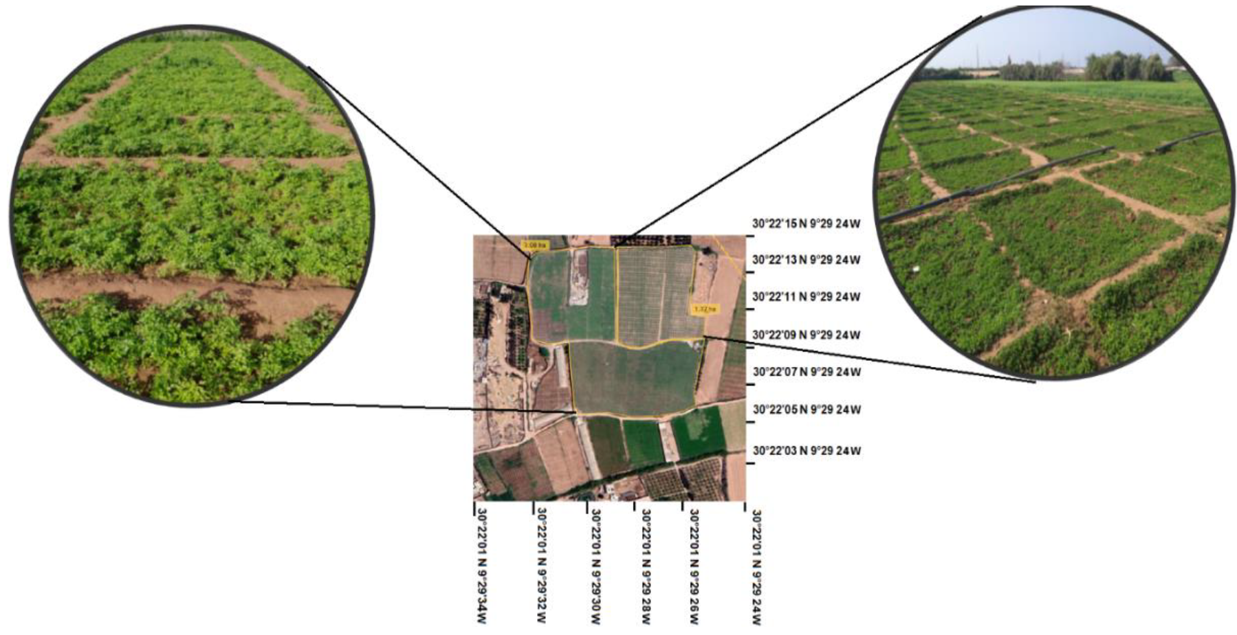
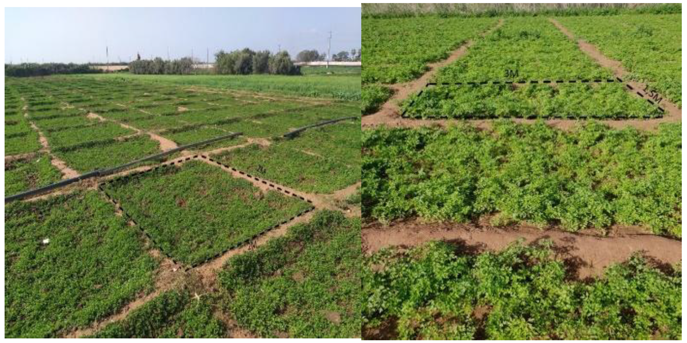
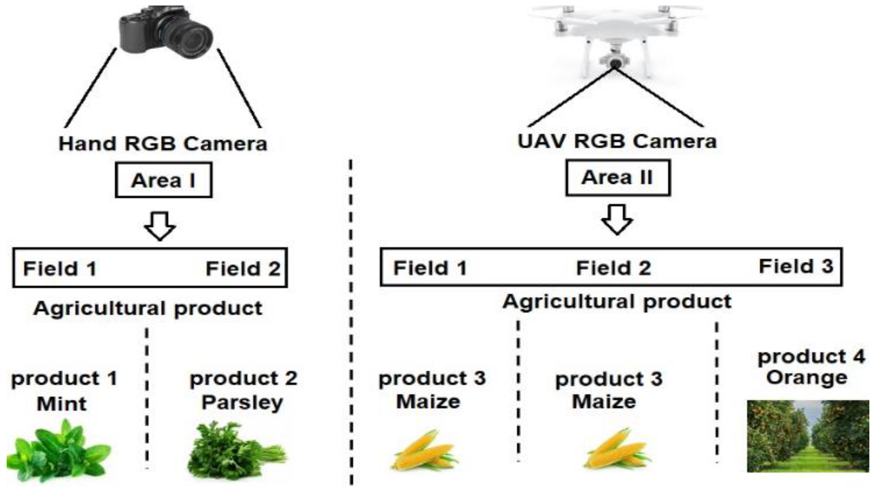
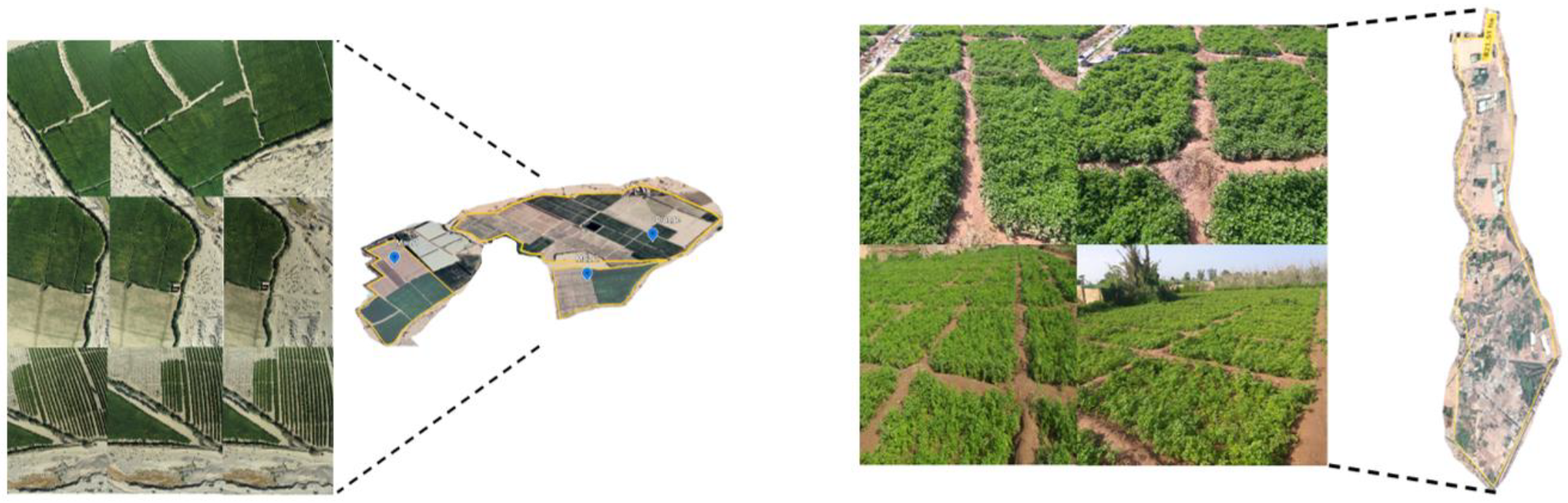
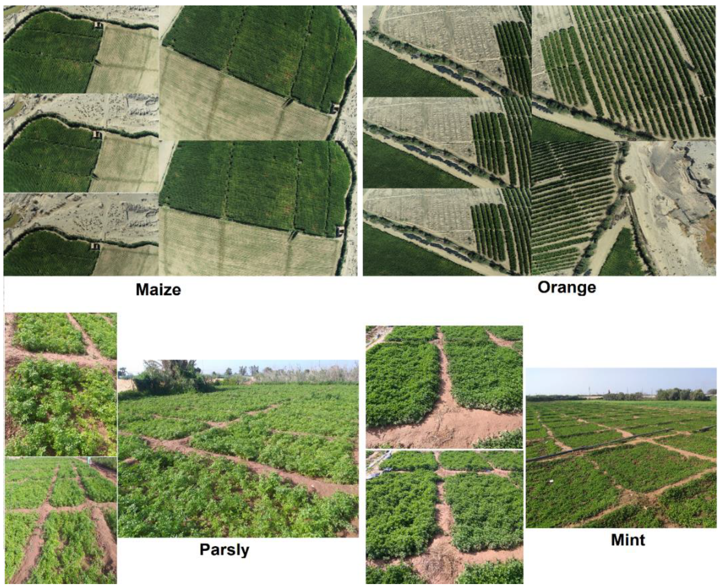
The data used in this paper is divided in two types—one collected by hand and the other collected by an unmanned aerial vehicle (UAV) type DJI. Figure 8 shows an example of the data used in our evaluation. The left image was collected by a UAV for the maize and orange products. On the other hand, the figure on the right is for mint and parsley. The choice of this agricultural product was made due to the popularity of this type of farm in the southern Moroccan region.

4.2. Sequential Implementation of the CPU-Based Algorith

The implementation on the CPUs of the used architecture is generally done in a sequential mode. This implementation, in our case, is based on the C/C++ language. After the temporal evaluation of the different blocks, we proceed to the distribution of each block in functional blocks, which reflect the various treatments used in the chosen block.

Table 7. Processing time of each block.

	Time (ms)
Blocks	Desktop	Jetson Nano	XU4	Raspberry
B1	33.9	96.2	120.5	222
B2	38.3	93	110	181
B3	61.4	127.2	155.9	300.8
Total	133.6	316.4	386.4	703.8

shows the processing time consumption of each block in our algorithm.

The time evaluation on several machines showed that the desktop consumes less time than the other tools used, giving a total time of 133.6 ms to process each image. In the other part, we have the two embedded systems, Jetson nano, and XU4, which consume, respectively, 316.4 and 386.4 ms for the processing of each image. These processing times are close, given the characteristics of each system. We also have the Raspberry card, which consumes 703.8 ms for each image. From the first analysis, we can say that blocks 1 and 3, which deal with blur detection and compression, consume more time than block 2, except in the desktop. This pushes us to analyze each block to see which part consumes more. The approach is to separate each block into functional blocks. These functional blocks take various tasks in the main block. In our case, we have tried to divide the first block into six functional blocks. 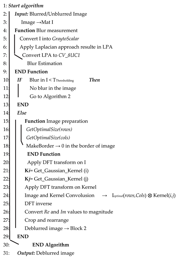Figure 9 shows the functional blocks used in our case based on block 1, which is responsible for blur detection and elimination as indicated in Algorithm 1.

The first functional block is dedicated to the blur test; this test is very important to avoid the processing if an image does not contain blur, which will decrease the processing time in some cases. The advantage, here, over the other techniques used is that, if we do not have blur, the algorithm will go directly to block 2 to calculate the indices. FB2 focuses on image preparation if we have blurred images. The third functional block is for the application of DFT to the image and the kernel. FB4 focuses on the convolution between the image and kernel DFT. FB5 for the Inverse Discrete Fourier Transform and finally FB6 for the magnitude and rearrangement to send the image to block 2 for indexes processing. Algorithm 1 shows the processing details of B1. This functional block separation will convert our algorithm into a functional block map which consists of 6 FB in block 1, giving a global view on the processing of this algorithm. 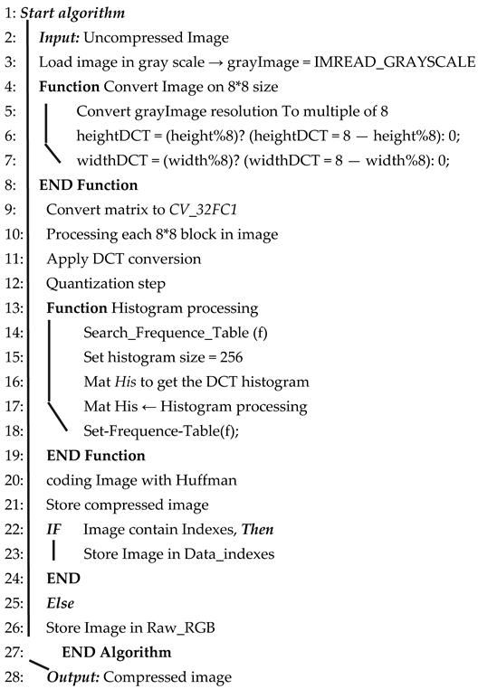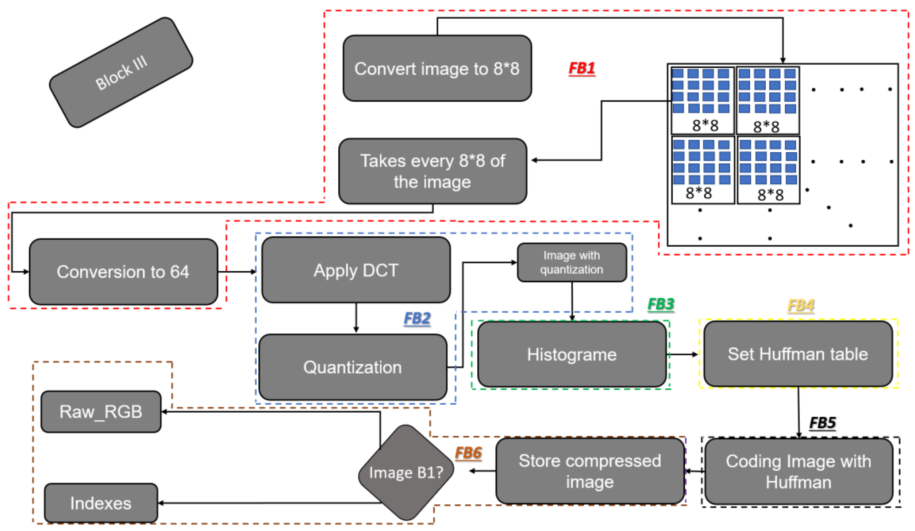Figure 10 shows block map 2.

In our case, the second block is described in [30]; for this reason, we focused only on blocks 1 and 3. Figure 10 shows that the compression algorithm is also divided into six functional blocks. FB1 focuses on searching optimal size to separate the image into 8*8 blocks and then convert it to 64 bits. FB2 takes care of the DCT application and the quantization, and FB3 for the histogram. Then FB4 and FB5 fill the Huffman table and the image coding based on these tables, respectively. The six functional blocks focus on the storage of the compressed images and the database management by applying a test to the image to see if it is an image that contains the different indices or a raw RGB image. After the specification of the different block functions, the time evaluation for the different blocks has to be applied in order to conclude which functional blocks consume more time. The time evaluation was based on the desktop, XU4, Jetson Nano, and Raspberry. 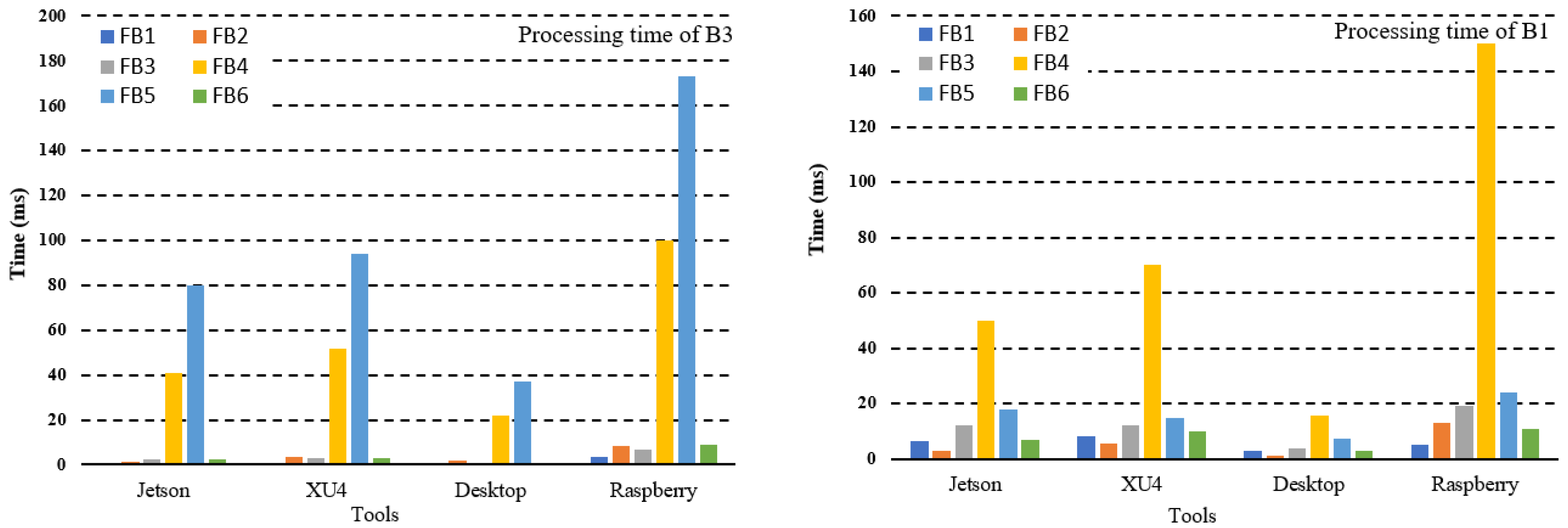Figure 11 shows the results obtained for each FB.

Figure 11 shows the results of the time evaluation for block 1 and 3; from the processing time analysis, we can conclude that in the case of block 1 (figure on the right), we have FB1 consuming 6.4 ms for Jetson Nano, 8.1 ms on the XU4 board, 3.1 ms for the desktop, and 5 ms for the Raspberry board. For FB2, we have 2.8 ms consumed by the Jetson Nano, 5.4 ms for XU4, 1.2 ms, and 13 ms for the desktop and Raspberry board, respectively.

FB3 occupies a processing time between 3.7 ms and 19 ms for the desktop and Raspberry and 12 ms for both the XU4 and Jetson Nano. Functional block 4 takes the largest percentage of time due to the conventional product between the image and the kernel, shown in the yellow curve. This increase in time reflects the fact that the function block selected for acceleration is FB4, which will reduce the total time of block 1. On the other hand, FB5 and FB6 consume less time compared to FB4. For block 3, the time evaluation showed that FB4 and FB5 consume more time compared to the other functional blocks, which requires an acceleration in these functional blocks. The time evaluation of the blocks was based on a sequence of 100 images in order to calculate the average processing time. Table 7 summarizes the different processing times obtained. From this table, we can conclude that the Jetson Nano card and the desktop are given the best results.

Although the desktop gives a lower time compared to other systems, the problem of this conventional machine is the power consumption and the high weight. In the same way, the Jetson nano card gives a difference of 70 ms compared to the XU4 card. This card indeed has a low cost, but it has a very high-power consumption compared to the XU4 and Raspberry cards. This does not reflect our interest because the study aims to build a reliable real-time system with low cost and low power consumption. In this case, the best choice is the XU4 and Raspberry board. The processing time analysis showed that the Raspberry board consumes more time by a factor of ×2.22 compared with XU4, which consumes 316 ms. That pushed us to select the XU4 board for the acceleration of the algorithm based on the exploitation of the CPU and GPU parts of this heterogeneous system. Due to the energy consumption in our case, we need to ensure the autonomy of the drone or the robot to provide the maximum processing capacity.

Table 8. Processing time of FBs.

	Time (ms)
Functional Block	Jetson	XU4	Desktop	Raspberry
		Block 3
FB1	0.17	0.136	0.094	3.3
FB2	1.5	3.7	2.03	8.5
FB3	2.2	2.9	0.317	7
FB4	41	52	22	100
FB5	80	94	37	173
FB6	2.4	3.2	0.034	9
		Block 1
FB1	6.4	8.1	3.1	5
FB2	2.8	5.4	1.2	13
FB3	12	12	3.7	19
FB4	50	70	15.7	150
FB5	18	15	7.3	24
FB6	7	10	2.9	11

shows the processing time of different FBs.

4.3. CPU-GPU Boarding Based OpenCL and OpenMP

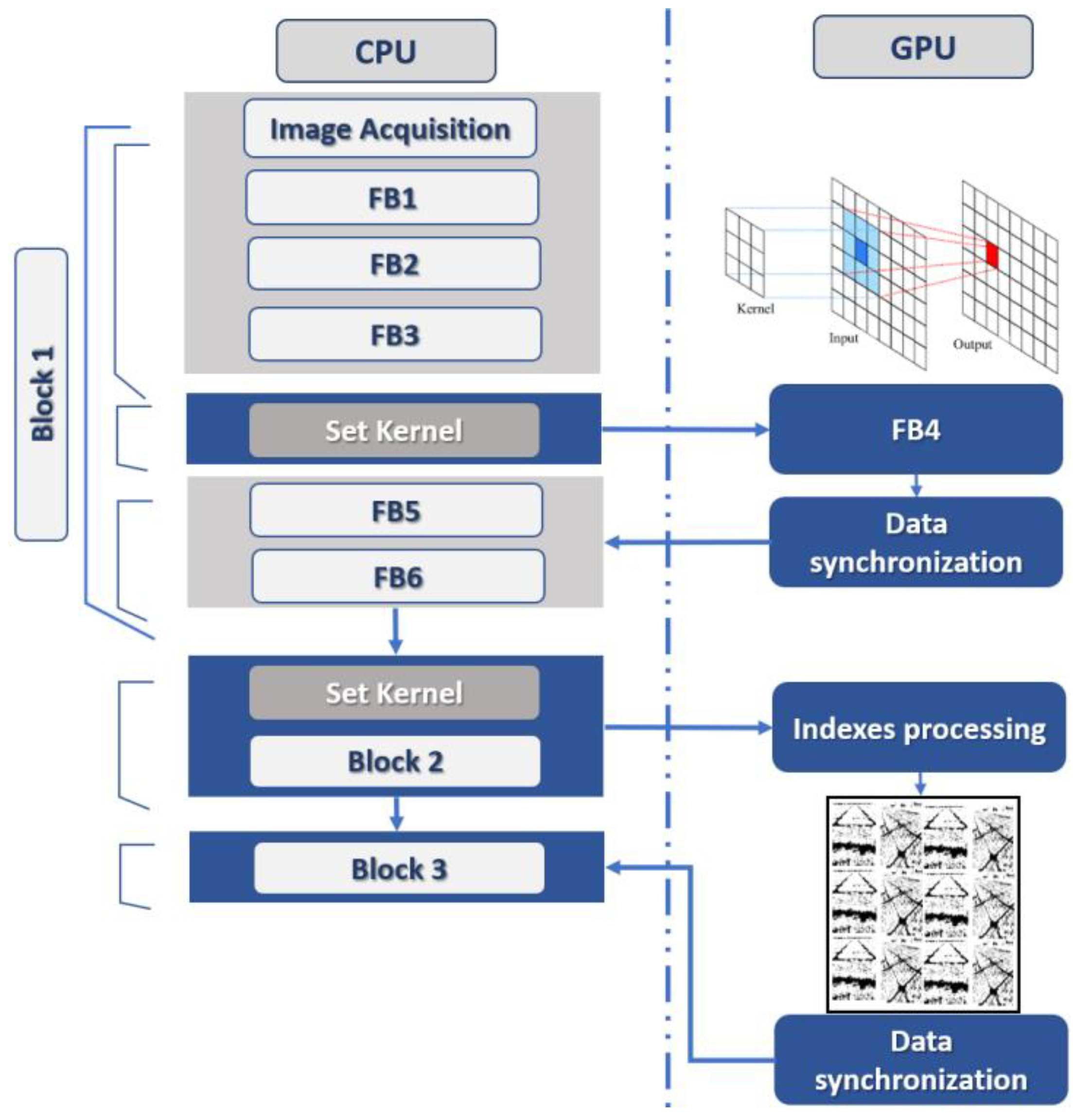
Our second implementation was based on OpenCL and OpenMP to accelerate the functional blocks that take most of the time. In our study, we used both languages to ensure the exploitation of the CPU part using OpenMP and the different GPU cores using OpenCL. The acceleration in the CPU of the XU4 board was used for the compression part and OpenCL for the blur elimination and index processing part. Figure 12 shows the implementation model based on the acceleration on the GPU part using OpenCL.

After the time evaluation shown in Table 8 and Figure 12, we have concluded that FB4 in block 1 consumes the most processing time. For this reason, we have opted to accelerate this FB in the GPU part of the board. Figure 13 shows that after FB3, we call the kernel for running on the GPU part; in this case, the CPU part provides the necessary data for the execution. Thus, we have accelerated block two, which also takes a lot of time. After the kernels have been executed, we move on to FB4 and FB5 in block 3, which has been accelerated in the CPU part via OpenMP. Figure 13 shows the results obtained.

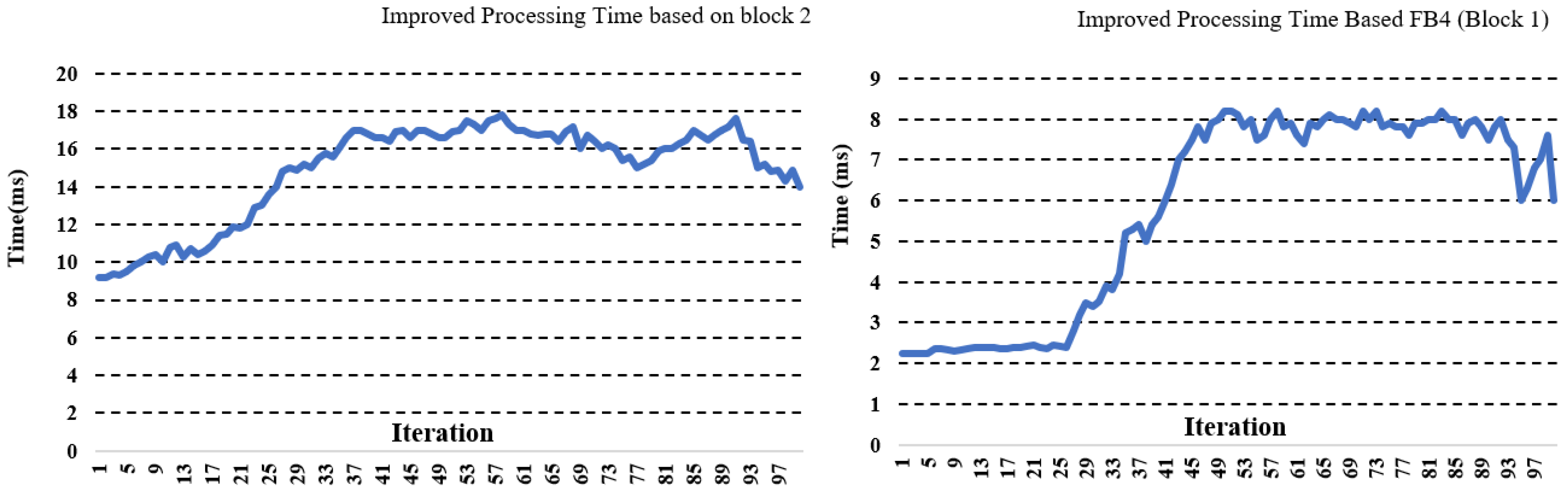
Figure 14 shows the temporal evaluation obtained based on a sequence of 100 images. The image on the left shows the block 2 time graph, which varies between a minimum value of 9.2 ms and a maximum value of 17.8 ms; after taking the average of the image sequence, we obtained a processing time of 14.89 ms for the handling of each image. This shows an improvement of ×7.3. compared to the sequential version, which consumes 110 ms. The time variation in the curves is due to the fact that each image contains a different information weight, which causes a variation in processing time. The image on the right also shows the processing time for 100 frames of FB 4 in block 1. The time varies between a minimum value of 2.24 ms and a maximum of 8.2 ms, which gives an average of 5.8 ms with an improvement ×12 compared to the sequential version, which consumes 70 ms. After improving blocks 1 and 2, we also enhanced block 3. Figure 14 and Figure 15 show the results obtained.

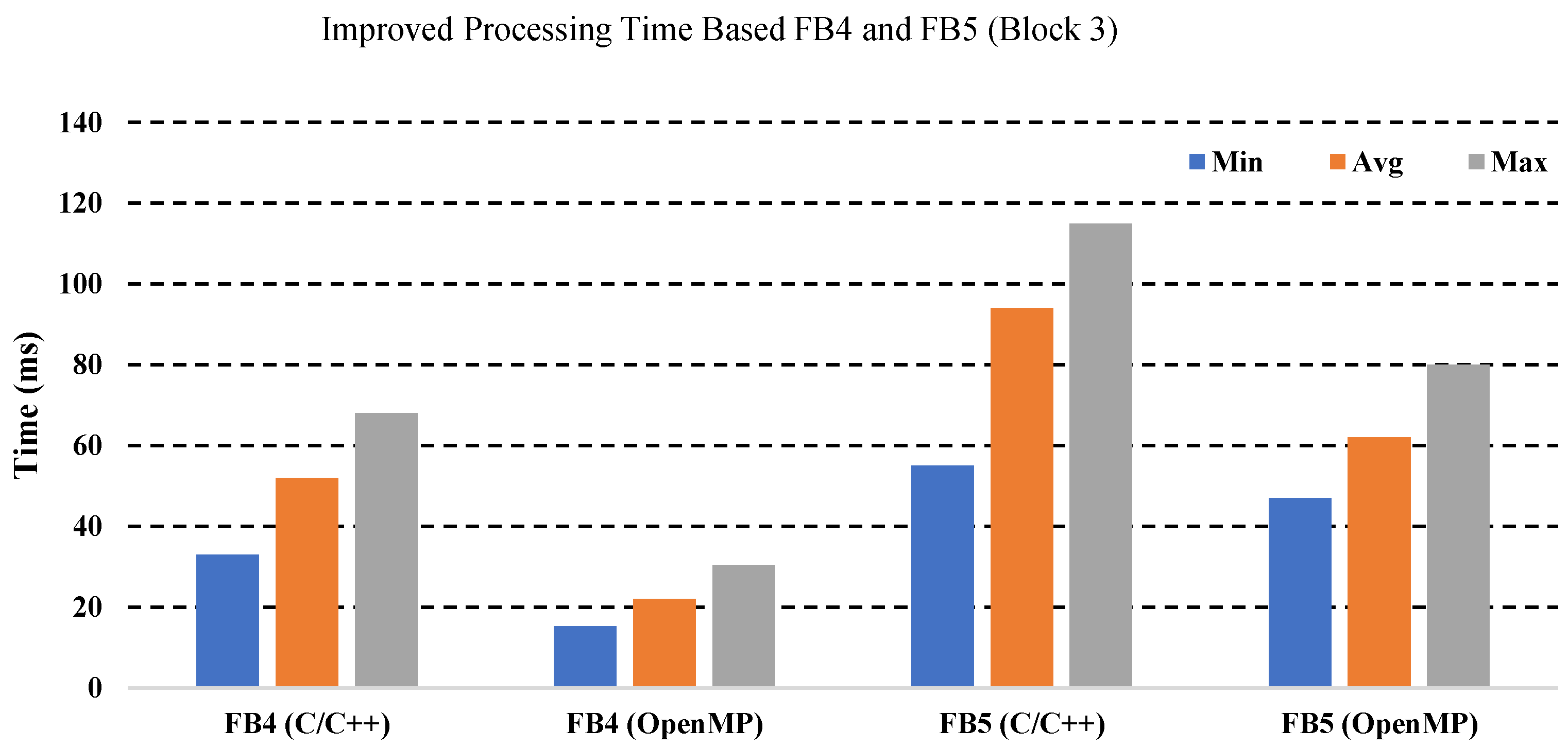
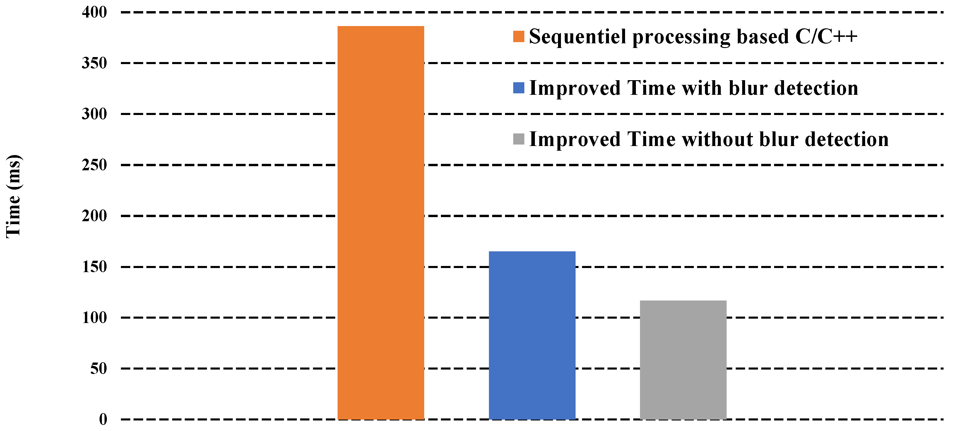
Figure 14 shows the processing time of FB4 and FB5 of block 3, which took the most processing time. In this context, we obtained an average of 22 ms compared to the sequential version, which consumes 52 ms for FB4 and 62 ms for FB5, and which consumes in the sequential version 94 ms. Figure 15 shows a comparison between the different times that include the sequential version and the improved version, as well as the case where we did not detect the blur in the image, so the algorithm moved directly to block 2 for the indices processing. This shows an improvement of ×3.3 in global processing time compared to the sequential version that took 386.4 ms. 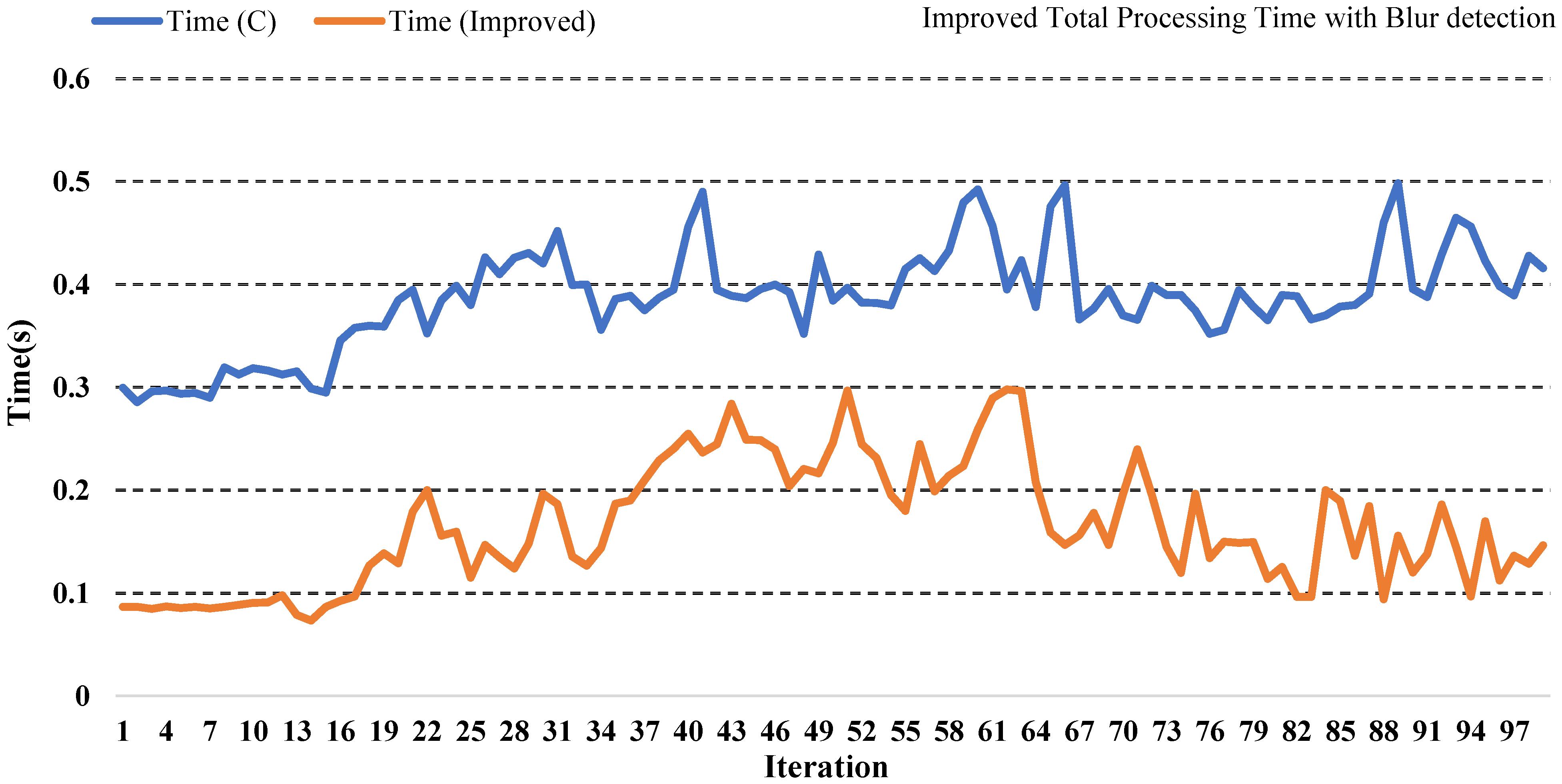Figure 16 shows the total time obtained between the improved and sequential versions based on 100 iterations.

We subsequently evaluated our implementation based on several resolutions to see the effect of the resolution on the processing time and the number of images processed.

Table 9. Global processing time with different resolution.

Resolution	CPU-GPU	Fps
640 × 480	3.21	311
1024 × 768	10.95	91
1600 × 1200	36.31	27
2048 × 1080	51.47	19
4096 × 2160	97.52	10
5472 × 3648	165.12	6

shows the result obtained.

Table 9 shows that using 640 × 480 resolution, we can achieve a processing rate of 311 frames/s, and 5472 × 3648 resolution, we can process 6 frames/s. The fact that the number of frames in this resolution is six is due to the high resolution of the images, but it is still sufficient, and it respects the real-time constraint. If we take as an example the most used cameras in precision agriculture, we find Red-Edge Mecasens or Parrot Sequoia, which have a time-lapse of two frames/s in the case of 1280 × 960 resolution for the different bands Red, Green, and Blue and 4608 × 3456 for the case of RGB, which means the various bands in the same image. Our algorithm respects the time constraint, which is 2 fps making the real-time processing.

5. Experimental Results from Real Area

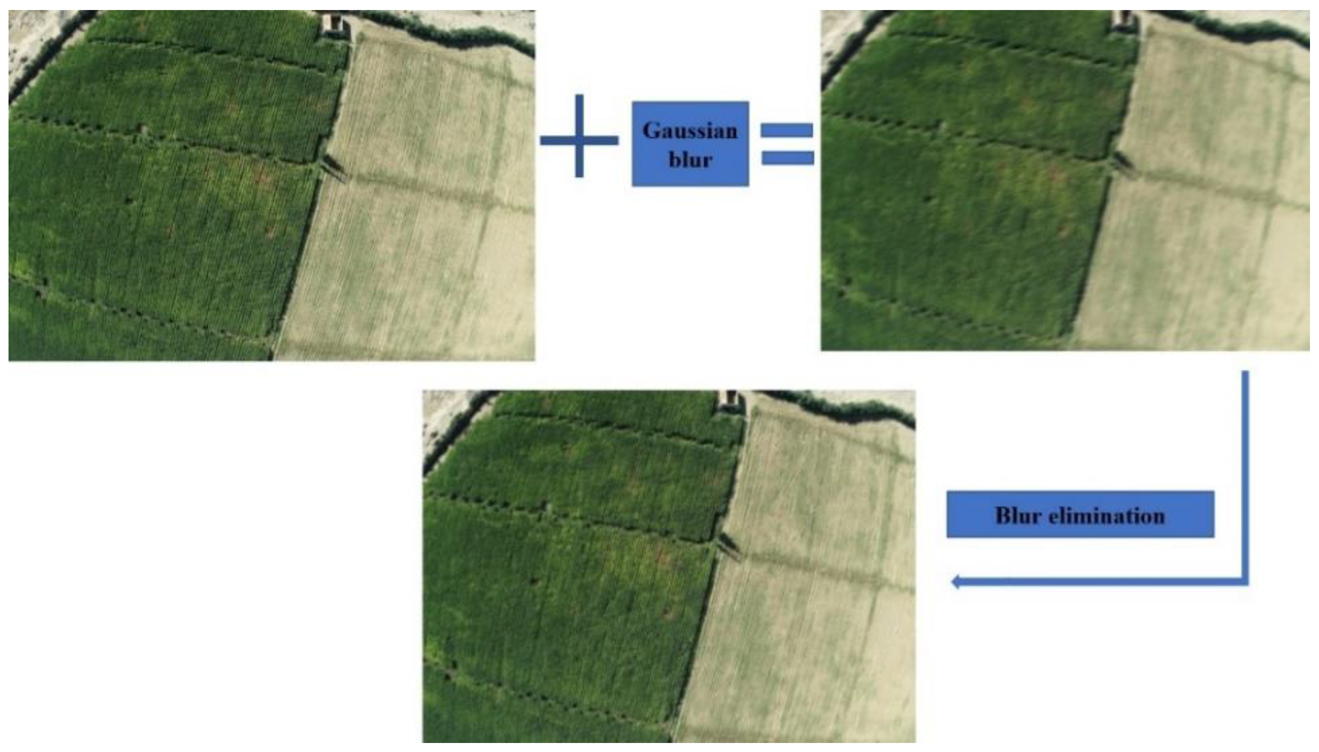
The temporal evaluation of our hybrid algorithm, which combines blur detection, index calculation, and image compression, has shown that we can use it in a real-time scenario. The compression results allowed us to reduce the image size by a factor of ×63. The decompression process to achieve the image construction was applied after the end of the sequence. This means that the decompression process is used after the global algorithm has processed all the images. For the blur detection, we tried to add a Gaussian blur to filter the image to see the result. Figure 17 shows the original image, with blur and after blur removal.

The indices evaluated in this work are the Normalized Green-Red Difference Index (NGRDI) and Visible Atmospherically Resistant Index (VARI). The choice of these indices is due to the robustness of the results given as well as their popularity in the field of precision agriculture. For this reason, we have evaluated both databases based on these indices. The images used in this evaluation are based on images collected by UAV and hand data. Figure 18 shows images from the database used in this work.

In Figure 18, we have the different images used in our evaluation. On the top left, we have an agricultural field of maize collected by a UAV; on the top right, we have a field of orange trees also collected by a UAV. We have a parsley field on the bottom left, and on the right, the mint field. These data were evaluated using the indices listed in Table 1; in our case, we chose the two indices NGRDI and VARI. 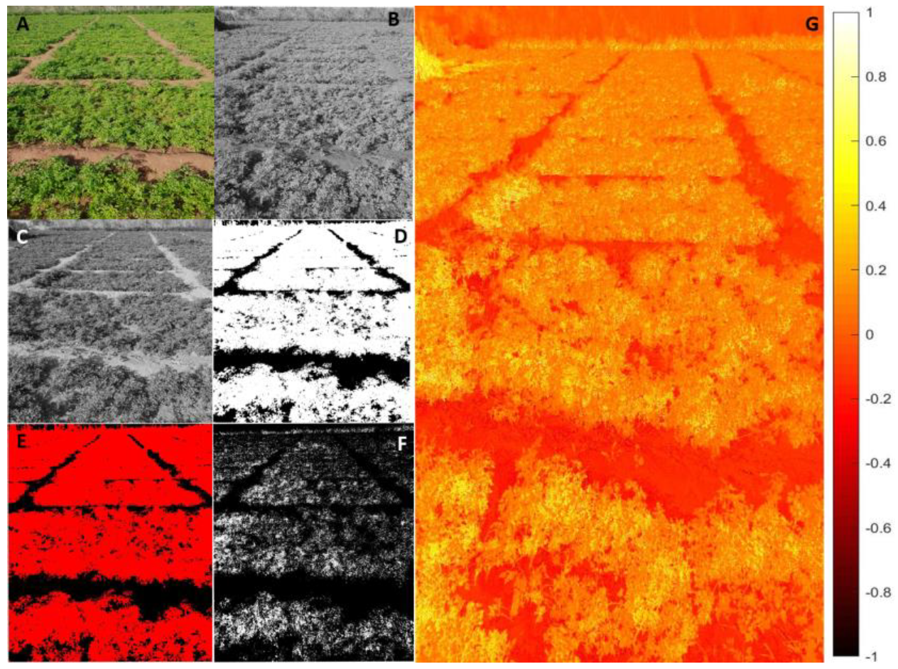Figure 19 shows the results obtained after the evaluation.

Figure 19 shows the evaluation of the NGRDI based on mint plants; image A shows the agricultural field, B is the green band, C is the red band, and D is the calculated index based on a threshold of 0.12. Images E and F show the same calculated index but we varied the threshold; in this case, we used a threshold of 0.45. Image G shows an index matrix generated by MATLAB to see the different values that exist in the image. Figure 20 shows the evaluation of parsley fields based on the NGRDI.

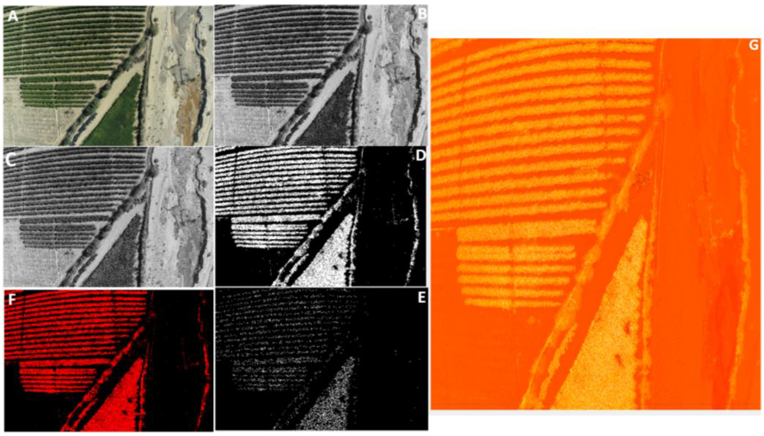
Thus, we have evaluated the orange plants as shown in Figure 21.

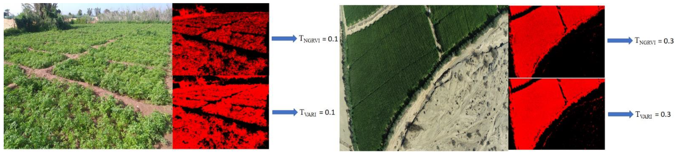
Figure 22 shows a comparison between NGRVI and VARI using parsley (in the left) and maize (in the right) plants. The image on the right shows the evaluation based on an image collected by UAV, and on the right, the database is collected by hand. The results showed that the VARI is more sensitive to vegetation than NGRVI based on the same threshold. Still, the results show that the VARI is robust to the sensitivity of the vegetation to be monitored.

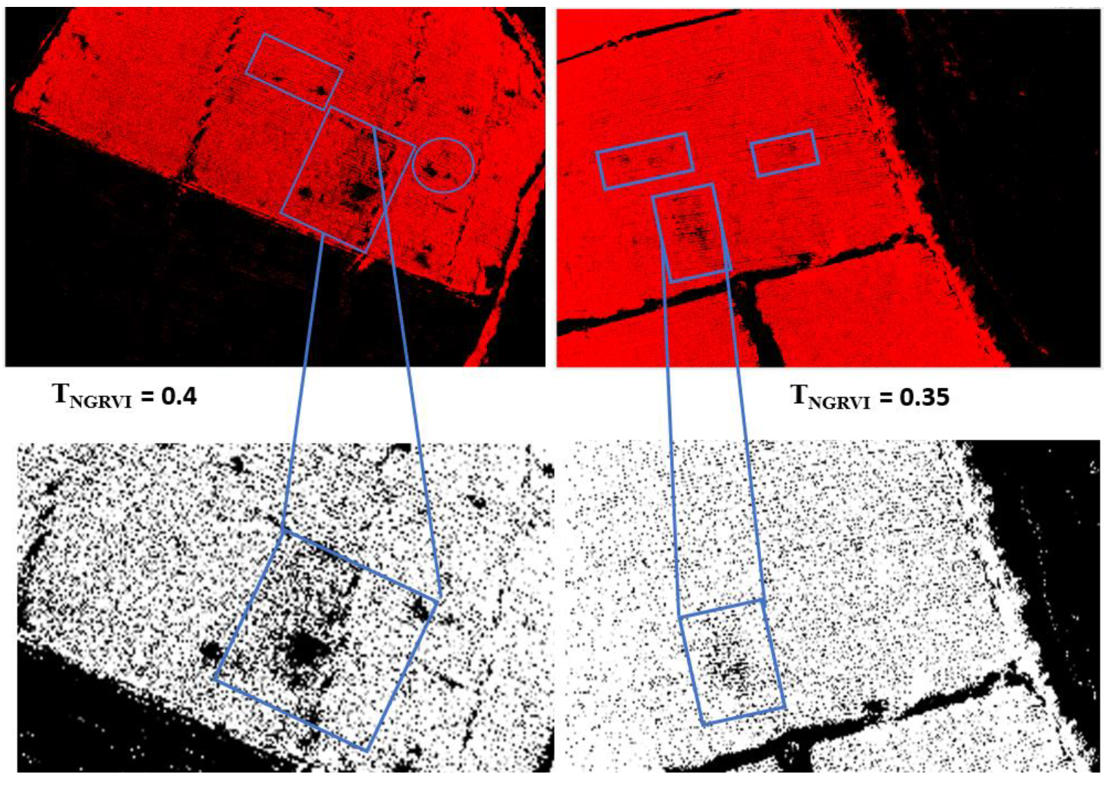
Figure 23 shows the interpretation of the index results, the image on the right shows that we have parts of the agricultural field with a low index after the threshold operation. The appropriate threshold comes with using a soil sensor to determine the suitable threshold for each plant. The blue squares show the soil parts with a low index, which implies a low vegetation cover that requires an intervention.

6. Conclusions and Future Work

Real-time monitoring of agricultural fields requires a robust monitoring system that satisfies the time constraint as well as the many other requirements. The hybrid algorithm proposed in this work tries to address the different constraints such as memory saturation during processing as well as blur detection due to camera movement during capture. The evaluation was based on several benchmarks to validate the algorithm’s implementation on several homogeneous low-cost embedded architectures such as the Raspberry board and heterogeneous ones such as Odroid XU4 and Jetson Nano. A Hardware/Software Co-Design study followed the validation of the algorithm to conclude that the XU4 board remains the best choice in terms of processing time, power consumption, and low cost. The evaluation results show that we can reach a processing performance up to 311 frames/s. Thus, the algorithm has been validated using our database collected with an RGB camera and a DJI Phantom Pro 4 drone. In terms of algorithmic complexity, the proposed algorithm has low complexity. The study of the temporal complexity has shown that the sequential implementation consumes a very high processing time that does not respect real-time. For this reason, hardware acceleration has been proposed to improve the proposed algorithm based on an acceleration factor of ×3.3 compared to sequential implementation. This acceleration is based on OpenCL and OpenMP language in XU4 embedded architecture. Future work aims to integrate precise localization algorithms to improve the quality of monitoring in agricultural fields based on multi-sensor fusion algorithms and accurate localization.

References

1. Lin, N.; Wang, X.; Zhang, Y.; Hu, X.; Ruan, J. Fertigation management for sustainable precision agriculture based on Internet of Things. J. Clean. Prod. 2020, 277, 124119. [Google Scholar] [CrossRef]
2. Sim, D.H.H.; Tan, I.A.W.; Lim, L.L.P.; Hameed, B.H. Encapsulated biochar-based sustained release fertilizer for precision agriculture: A review. J. Clean. Prod. 2021, 303, 127018. [Google Scholar] [CrossRef]
3. Brisco, B.; Brown, R.J.; Hirose, T.; McNairn, H.; Staenz, K. Precision Agriculture and the Role of Remote Sensing: A Review. Can. J. Remote Sens. 1998, 24, 315–327. [Google Scholar] [CrossRef]
4. Liu, W.; Shao, X.-F.; Wu, C.-H.; Qiao, P. A systematic literature review on applications of information and communication technologies and blockchain technologies for precision agriculture development. J. Clean. Prod. 2021, 298, 126763. [Google Scholar] [CrossRef]
5. Srbinovska, M.; Gavrovski, C.; Dimcev, V.; Krkoleva, A.; Borozan, V. Environmental parameters monitoring in precision agriculture using wireless sensor networks. J. Clean. Prod. 2015, 88, 297–307. [Google Scholar] [CrossRef]
6. Li, D.; Wang, R.; Xie, C.; Liu, L.; Zhang, J.; Li, R.; Wang, F.; Zhou, M.; Liu, W. A Recognition Method for Rice Plant Diseases and Pests Video Detection Based on Deep Convolutional Neural Network. Sensors 2020, 20, 578. [Google Scholar] [CrossRef] [PubMed] [Green Version]
7. Yu, H.; Liu, K.; Bai, Y.; Luo, Y.; Wang, T.; Zhong, J.; Liu, S.; Bai, Z. The Agricultural Planting Structure Adjustment based on Water Footprint and Multi-objective optimisation models in China. J. Clean. Prod. 2021, 297, 126646. [Google Scholar] [CrossRef]
8. Dey, K.; Shekhawat, U. Blockchain for sustainable e-agriculture: Literature review, architecture for data management, and implications. J. Clean. Prod. 2021, 316, 128254. [Google Scholar] [CrossRef]
9. Shadrin, D.; Menshchikov, A.; Ermilov, D.; Somov, A. Designing Future Precision Agriculture: Detection of Seeds Germination Using Artificial Intelligence on a Low-Power Embedded System. IEEE Sens. J. 2019, 19, 11573–11582. [Google Scholar] [CrossRef]
10. Rodríguez, J.; Lizarazo, I.; Prieto, F.; Angulo-Morales, V. Assessment of potato late blight from UAV-based multispectral imagery. Comput. Electron. Agric. 2021, 184, 106061. [Google Scholar] [CrossRef]
11. Hassan, M.A.; Yang, M.; Rasheed, A.; Yang, G.; Reynolds, M.; Xia, X.; Xiao, Y.; He, Z. A rapid monitoring of NDVI across the wheat growth cycle for grain yield prediction using a multi-spectral UAV platform. Plant Sci. 2019, 282, 95–103. [Google Scholar] [CrossRef] [PubMed]
12. Wang, A.; Xu, Y.; Wei, X.; Cui, B. Semantic Segmentation of Crop and Weed using an Encoder-Decoder Network and Image Enhancement Method under Uncontrolled Outdoor Illumination. IEEE Access 2020, 8, 81724–81734. [Google Scholar] [CrossRef]
13. Abouzahir, S.; Sadik, M.; Sabir, E. Bag-of-visual-words-augmented Histogram of Oriented Gradients for efficient weed detection. Biosyst. Eng. 2021, 202, 179–194. [Google Scholar] [CrossRef]
14. Tu, S.; Pang, J.; Liu, H.; Zhuang, N.; Chen, Y.; Zheng, C.; Wan, H.; Xue, Y. Passion fruit detection and counting based on multiple scale faster R-CNN using RGB-D images. Precis. Agric. 2020, 21, 1072–1091. [Google Scholar] [CrossRef]
15. Hummel, R.A.; Kimia, B.; Zucker, S.W. Deblurring Gaussian blur. Comput. Vis. Graph. Image Process. 1987, 38, 66–80. [Google Scholar] [CrossRef]
16. Motohka, T.; Nasahara, K.N.; Oguma, H.; Tsuchida, S. Applicability of Green-Red Vegetation Index for Remote Sensing of Vegetation Phenology. Remote Sens. 2010, 2, 2369–2387. [Google Scholar] [CrossRef] [Green Version]
17. Hunt, E.R.; Cavigelli, M.; Daughtry, C.S.T.; Mcmurtrey, J.E.; Walthall, C.L. Evaluation of Digital Photography from Model Aircraft for Remote Sensing of Crop Biomass and Nitrogen Status. Precis. Agric. 2005, 6, 359–378. [Google Scholar] [CrossRef]
18. Bendig, J.; Yu, K.; Aasen, H.; Bolten, A.; Bennertz, S.; Broscheit, J.; Gnyp, M.L.; Bareth, G. Combining UAV-based plant height from crop surface models, visible, and near infrared vegetation indices for biomass monitoring in barley. Int. J. Appl. Earth Obs. Geoinf. 2015, 39, 79–87. [Google Scholar] [CrossRef]
19. Gitelson, A.A.; Kaufman, Y.J.; Stark, R.; Rundquist, D. Novel algorithms for remote estimation of vegetation fraction. Remote Sens. Environ. 2002, 80, 76–87. [Google Scholar] [CrossRef] [Green Version]
20. Ranđelović, P.; Đorđević, V.; Milić, S.; Balešević-Tubić, S.; Petrović, K.; Miladinović, J.; Đukić, V. Prediction of Soybean Plant Density Using a Machine Learning Model and Vegetation Indices Extracted from RGB Images Taken with a UAV. Agronomy 2020, 10, 1108. [Google Scholar] [CrossRef]
21. Shadrin, D.; Menshchikov, A.; Somov, A.; Bornemann, G.; Hauslage, J.; Fedorov, M. Enabling Precision Agriculture Through Embedded Sensing with Artificial Intelligence. IEEE Trans. Instrum. Meas. 2020, 69, 4103–4113. [Google Scholar] [CrossRef]
22. Ericson, S.K.; Åstrand, B.S. Analysis of two visual odometry systems for use in an agricultural field environment. Biosyst. Eng. 2018, 166, 116–125. [Google Scholar] [CrossRef] [Green Version]
23. Burgos-Artizzu, X.P.; Ribeiro, A.; Guijarro, M.; Pajares, G. Real-time image processing for crop/weed discrimination in maize fields. Comput. Electron. Agric. 2011, 75, 337–346. [Google Scholar] [CrossRef] [Green Version]
24. Marcial-Pablo, M.d.J.; Gonzalez-Sanchez, A.; Jimenez-Jimenez, S.I.; Ontiveros-Capurata, R.E.; Ojeda-Bustamante, W. Estimation of vegetation fraction using RGB and multispectral images from UAV. Int. J. Remote Sens. 2019, 40, 420–438. [Google Scholar] [CrossRef]
25. Sumesh, K.C.; Ninsawat, S.; Som-ard, J. Integration of RGB-based vegetation index, crop surface model and object-based image analysis approach for sugarcane yield estimation using unmanned aerial vehicle. Comput. Electron. Agric. 2021, 180, 105903. [Google Scholar] [CrossRef]
26. De Swaef, T.; Maes, W.H.; Aper, J.; Baert, J.; Cougnon, M.; Reheul, D.; Steppe, K.; Roldán-Ruiz, I.; Lootens, P. Applying RGB- and Thermal-Based Vegetation Indices from UAVs for High-Throughput Field Phenotyping of Drought Tolerance in Forage Grasses. Remote Sens. 2021, 13, 147. [Google Scholar] [CrossRef]
27. Chebrolu, N.; Lottes, P.; Schaefer, A.; Winterhalter, W.; Burgard, W.; Stachniss, C. Agricultural robot dataset for plant classification, localization and mapping on sugar beet fields. Int. J. Rob. Res. 2017, 36, 1045–1052. [Google Scholar] [CrossRef] [Green Version]
28. Potena, C.; Khanna, R.; Nieto, J.; Siegwart, R.; Nardi, D.; Pretto, A. AgriColMap: Aerial-Ground Collaborative 3D Mapping for Precision Farming. IEEE Robot. Autom. Lett. 2019, 4, 1085–1092. [Google Scholar] [CrossRef] [Green Version]
29. Zhou, X.; Yang, L.; Wang, W.; Chen, B. UAV Data as an Alternative to Field Sampling to Monitor Vineyards Using Machine Learning Based on UAV/Sentinel-2 Data Fusion. Remote Sens. 2021, 13, 457. [Google Scholar] [CrossRef]
30. Saddik, A.; Latif, R.; Elhoseny, M.; El Ouardi, A. Real-time evaluation of different indexes in precision agriculture using a heterogeneous embedded system. Sustain. Comput. Inform. Syst. 2021, 30, 100506. [Google Scholar] [CrossRef]
31. Saddik, A.; Latif, R.; El Ouardi, A. Low-Power FPGA Architecture Based Monitoring Applications in Precision Agriculture. J. Low Power Electron. Appl. 2021, 11, 39. [Google Scholar] [CrossRef]
32. Saddik, A.; Latif, R.; El Ouardi, A.; Elhoseny, M.; Khelifi, A. Computer development based embedded systems in precision agriculture: Tools and application. Acta Agric. Scand. B Soil Plant Sci. 2022, 1–23. [Google Scholar] [CrossRef]
33. Yang, F.; Huang, Y.; Luo, Y.; Li, L.; Li, H. Robust Image Restoration for Motion Blur of Image Sensors. Sensors 2016, 16, 845. [Google Scholar] [CrossRef] [PubMed] [Green Version]
34. Hatim, A.; Belkouch, S.; Benslimane, A.; Hassani, M.M.; Sadiki, T. Efficient architecture for direct 8 × 8 2D DCT computations with earlier zigzag ordering. Multimed. Tools Appl. 2016, 75, 6121–6141. [Google Scholar] [CrossRef]
35. Lucy, L.B. An iterative technique for the rectification of observed distributions. Astron. J. 1974, 79, 745. [Google Scholar] [CrossRef] [Green Version]
36. Richardson, W.H. Bayesian-based iterative method of image restoration. JoSA 1972, 62, 55–59. [Google Scholar] [CrossRef]
37. Marks, L.D. Wiener-filter enhancement of noisy HREM images. Ultramicroscopy 1996, 62, 43–52. [Google Scholar] [CrossRef]
38. Rao, K.-R.; Kim, D.-N.; Hwang, J.-J. Discrete Fourier Transform. In Fast Fourier Transform—Algorithms and Applications; Springer: Dordrecht, The Netherlands, 2010. [Google Scholar] [CrossRef]
Figure 1. Souss Massa agricultural area.
Sustainability 14 02521 g001
Figure 2. Localization of the mint and parsley fields.
Sustainability 14 02521 g002
Figure 3. Mint and parsley ponds.
Sustainability 14 02521 g003
Figure 4. Localization of maize and orange area.
Sustainability 14 02521 g004
Figure 5. Maize and orange area.
Sustainability 14 02521 g005
Figure 6. Different agricultural products used in our study based on mint, parsley, oranges, and maize.
Sustainability 14 02521 g006
Figure 7. Global algorithm overview.
Sustainability 14 02521 g007
Figure 8. Used data.
Sustainability 14 02521 g008
Figure 9. Functional block flow of blur detection algorithm.
Sustainability 14 02521 g009
Figure 10. Functional block flow of compression algorithm.
Sustainability 14 02521 g010
Figure 11. Processing time of each functional block: sequential implementation.
Sustainability 14 02521 g011
Figure 12. CPU-GPU implementation based on OpenCL.
Sustainability 14 02521 g012
Figure 13. GPU processing time based on OpenCL.
Sustainability 14 02521 g013
Figure 14. CPU processing time based on OpenMP.
Sustainability 14 02521 g014
Figure 15. Processing time comparison.
Sustainability 14 02521 g015
Figure 16. Processing time comparison with global processing time in XU4 embedded system.
Sustainability 14 02521 g016
Figure 17. Blur elimination result.
Sustainability 14 02521 g017
Figure 18. Used data based on mint, maize, orange, and parsley.
Sustainability 14 02521 g018
Figure 19. Evaluation of NGRDI based on mint. ((A) represents RGB image; (B) is green band; (C) is red band; (D) is the NGRDI processing; (E) is NGRDI processing but using a modified thresholding; (F) represent the same index but using red color; (G) is the NGRDI processing using a MATLAB.)
Sustainability 14 02521 g019
Figure 20. Evaluation of NGRDI based on parsley. ((A) represents RGB image; (B) is green band; (C) is red band; (D) is NGRDI processing but using a modified thresholding; (E) represent the same index but using red color; (F) is the NGRDI processing; (G) is the NGRDI processing using a MATLAB.)
Sustainability 14 02521 g020
Figure 21. Evaluation of NGRDI based on orange. ((A) represents the original RGB image, (B) the red band of the image, and (C) the green band. Image (D) shows the binary image of the NGRDI with a threshold of 0.35, as same for image (F), by coloring the image in red for the regions with an index of 0.35. For image (E), we have modified the threshold based on 0.5 this time instead of 0.35. Image (G) presents a matrix data of the index.)
Sustainability 14 02521 g021
Figure 22. Result comparison between NGRVI and VARI based on parsley and maize.
Sustainability 14 02521 g022
Figure 23. Result interpretation of NGRVI.
Sustainability 14 02521 g023