
Estimating per Capita Primary Energy Consumption Using a Novel Fractional Gray Bernoulli Model


Abstract
:1. Introduction
2. Methodology
2.1. Gray Bernoulli Models: NGBM (1,1) and FAGM (1,1,)
2.2. Description of the GFGBM (1,1,)
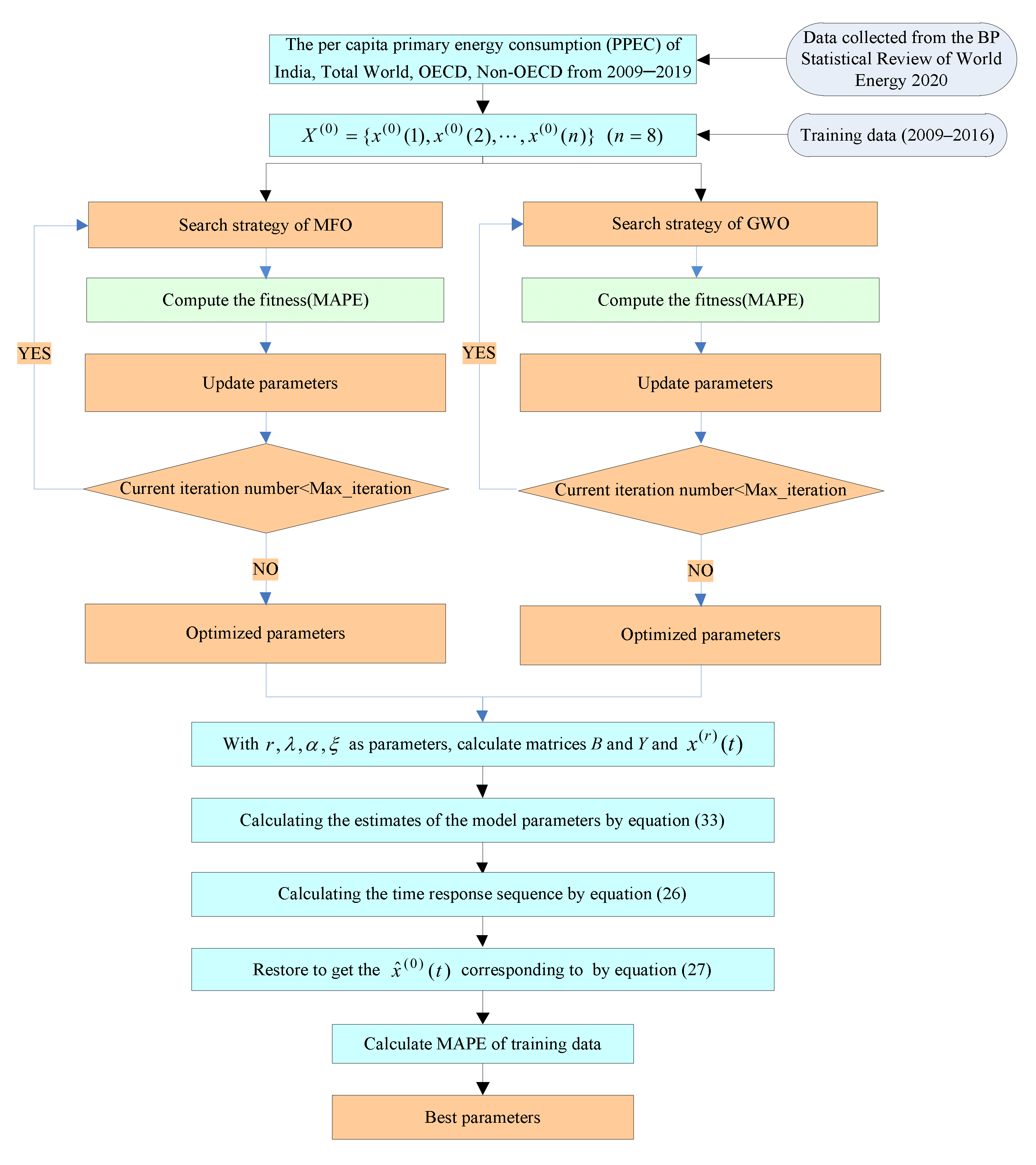
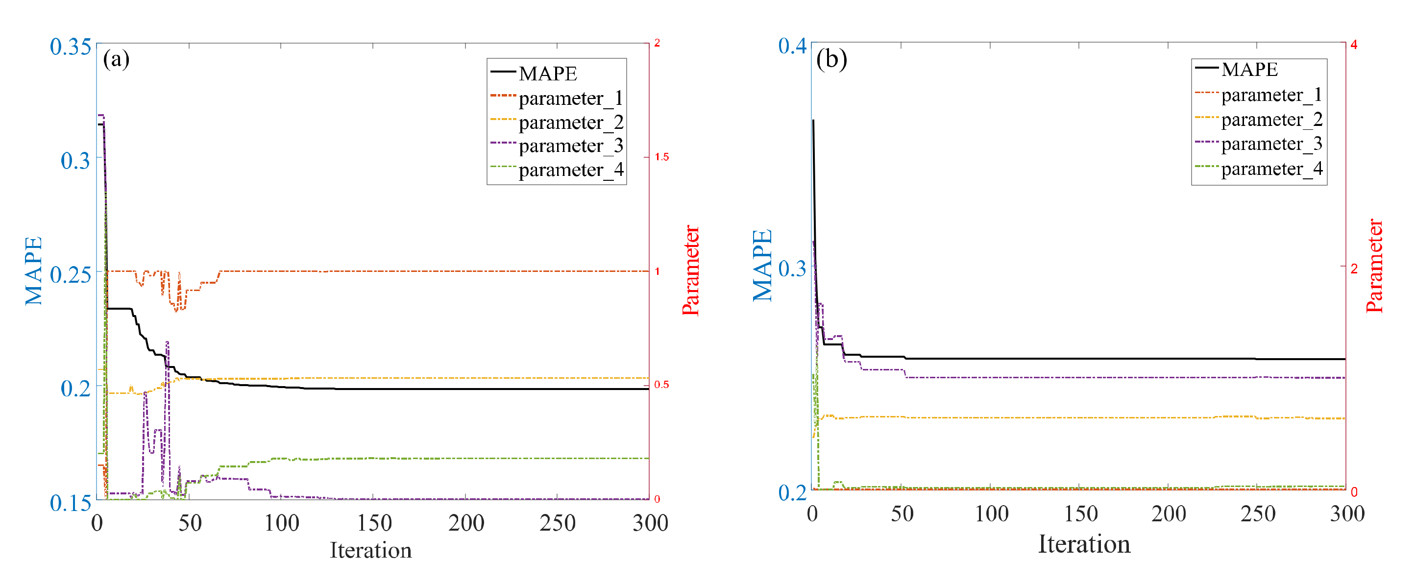
2.3. Parameter Estimation for the GFGBM (1,1,)
2.4. The Properties of the GFGBM (1,1,)
- Scenario 1: For , and or , the GFGBM (1,1,) can be converted into the GM (1,1) [22].
- Scenario 2: For , the GFGBM (1,1,) can be converted into the FGM (1,1) [51].
- Scenario 3: For , the GFGBM (1,1,) can be converted into the NGM (1,1,k,c) [52].
- Scenario 4: For , the GFGBM (1,1,) can be converted into the FNGM [27].
- Scenario 5: For , the GFGBM (1,1,) can be converted into the GMP (1,1,N) [38].
- Scenario 6: For or , the GFGBM (1,1,) can be converted into the FANGBM (1,1) [30].
- Scenario 7: For , the GFGBM (1,1,) can be converted into the NGBM (1,1,k,c) [47].
- Scenario 8: For , the GFGBM (1,1,) can be converted into the FGPM (1,1,) [31].
2.5. Error Metric
2.6. Validation of the GFGBM (1,1,)
3. Results and Discussion
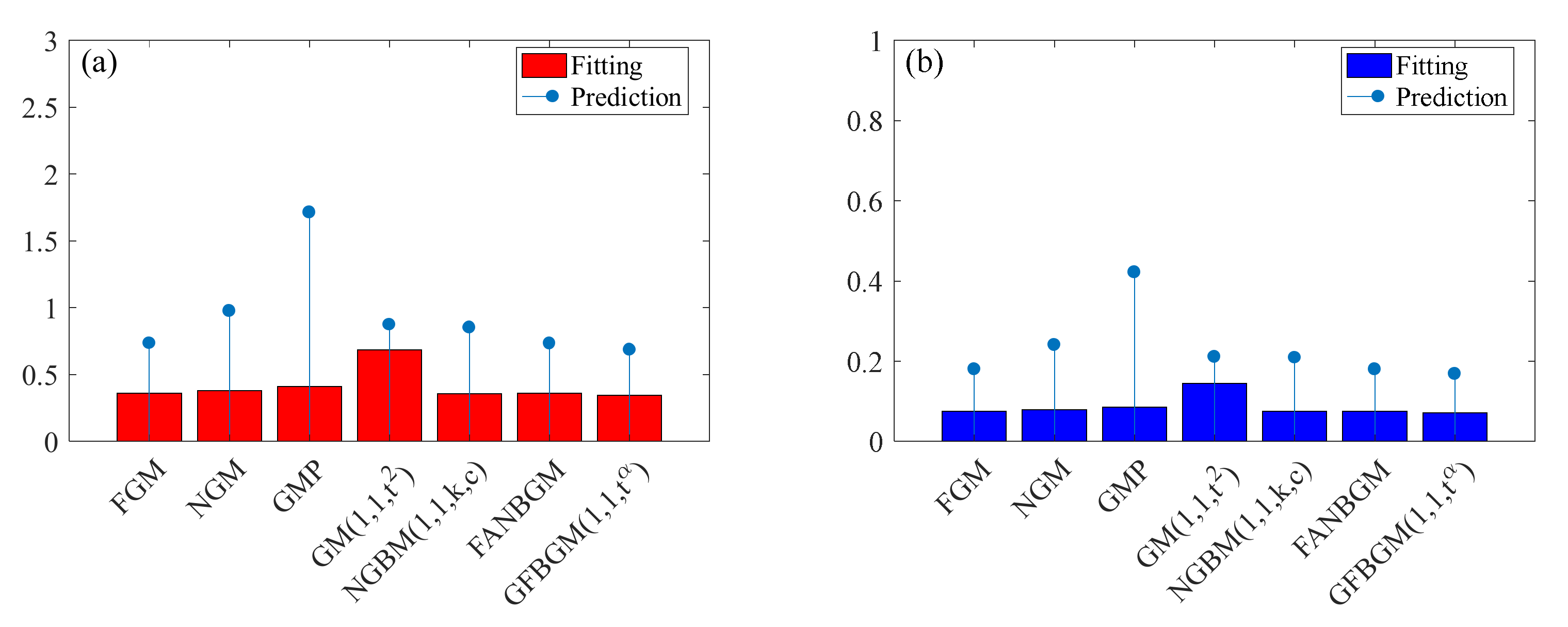
3.1. Model Comparison Results of Four Economies
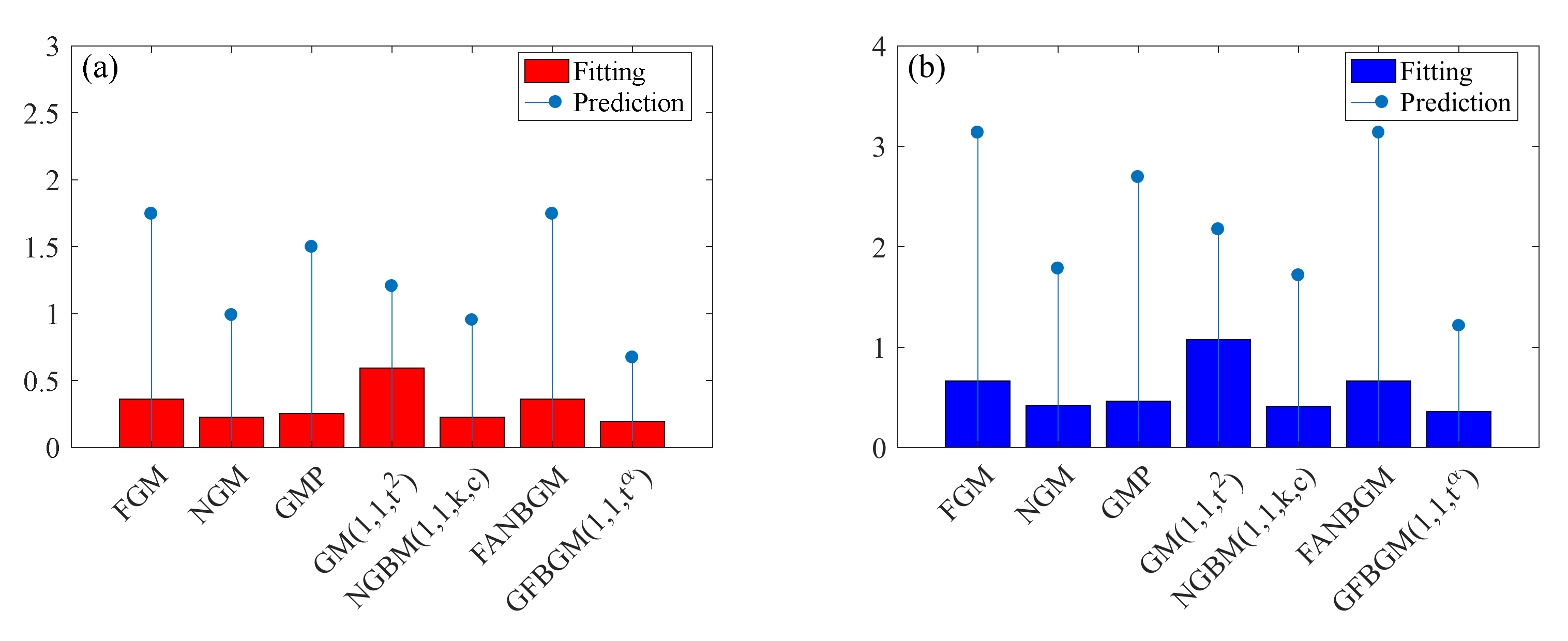
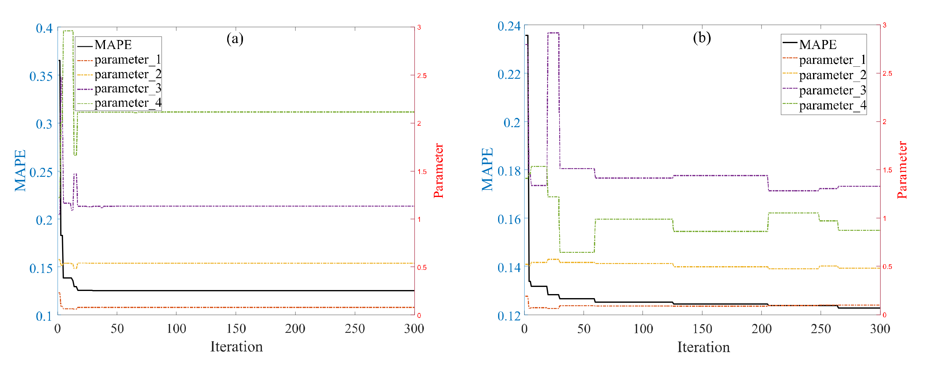
3.1.1. PPEC of India
3.1.2. PPEC of the World
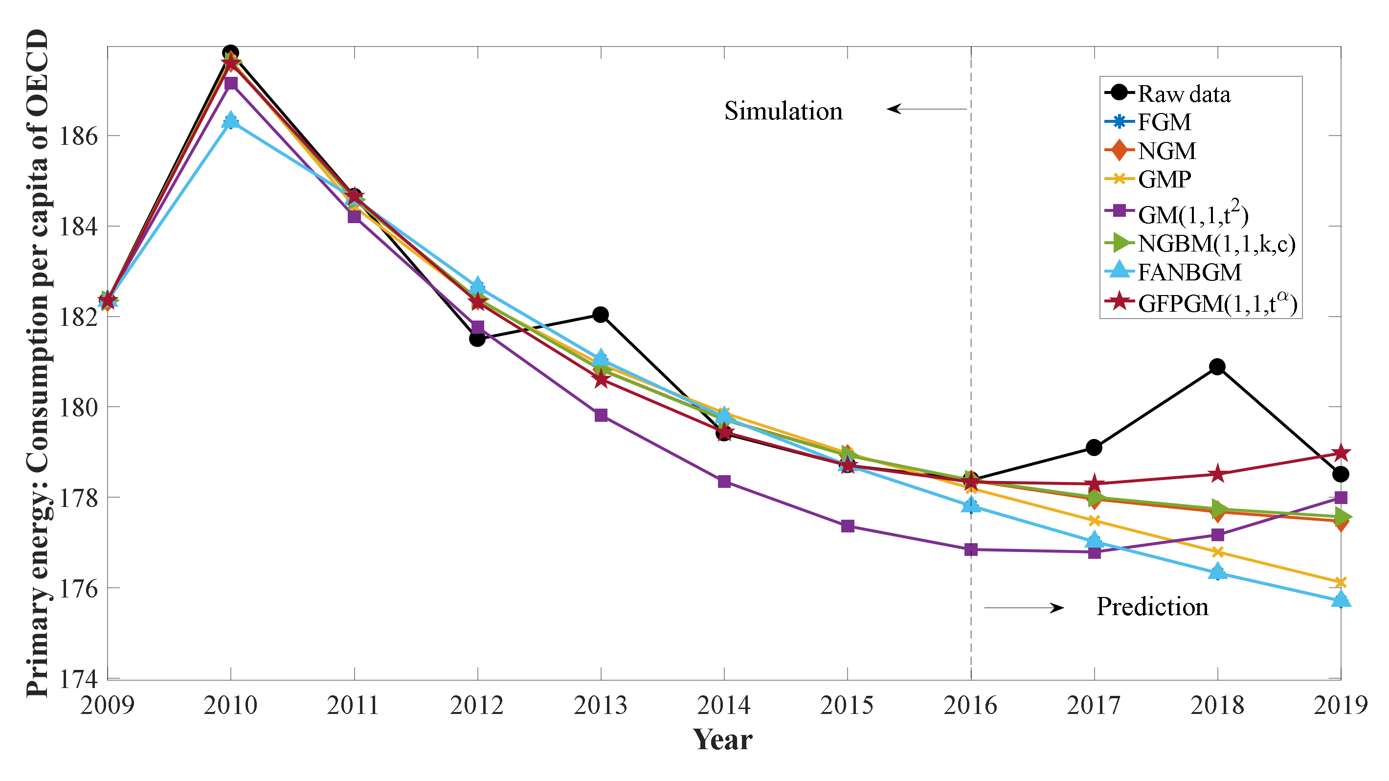
3.1.3. PPEC of OECD Countries
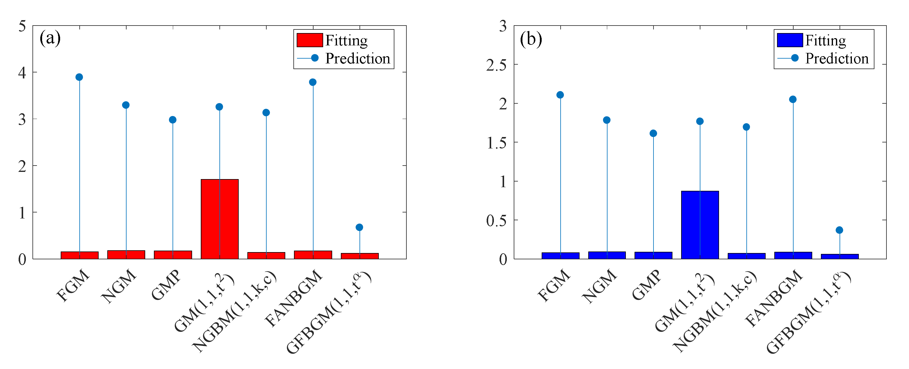
3.1.4. PPEC of Non-OECD
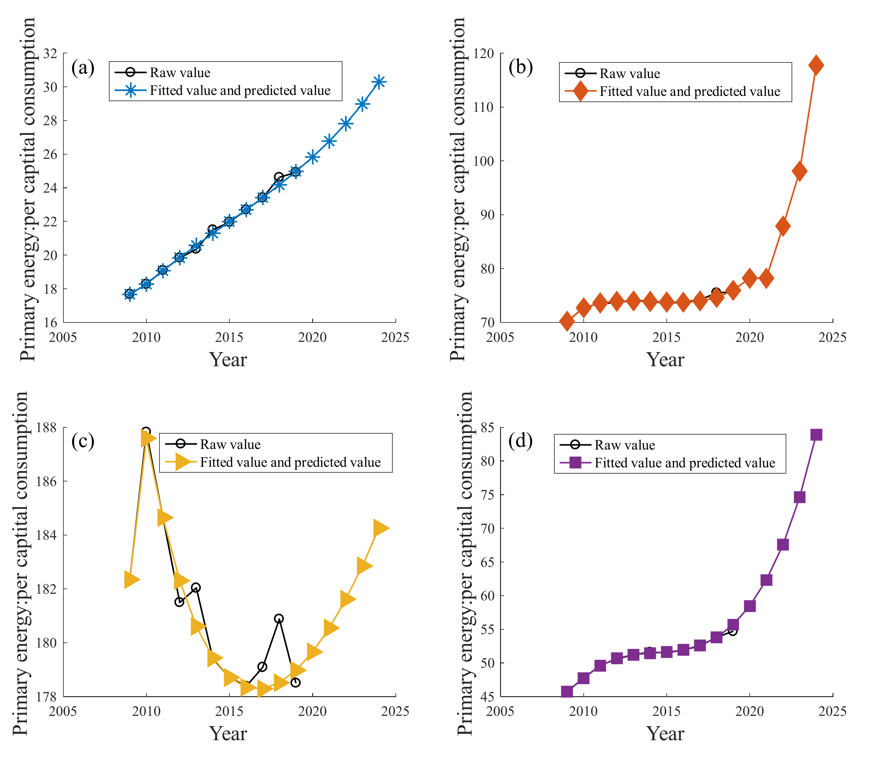
3.2. Forecasting the PPEC over the Next 5 Years
4. Conclusions
Author Contributions
Funding
Institutional Review Board Statement
Informed Consent Statement
Data Availability Statement
Conflicts of Interest
Nomenclature
| PPEC | Per capita primary energy consumption |
| FOA | Fractional order (r-order) accumulation |
| IFOA | Inverse fractional order (r-order) accumulation |
| Original series | |
| First-order accumulated series | |
| GM (1,1) | Basic gray model |
| FGM (1,1) | Fractional gray model |
| NGM (1,1) | Nonlinear gray model |
| GMP (1,1,2) | Gray model with polynomial term |
| GM (1,1,) | Gray model with time power |
| NGBM (1,1) | Nonlinear gray Bernoulli model |
| FANGBM (1,1) | Fractional nonlinear gray Bernoulli model |
| FPGM(1,1,) | Fractional gray polynomial model with time power term |
| GFGBM (1,1,) | Fractional gray Bernoulli model with time power term |
| GWO | Gray wolf optimization |
| MFO | Moth flame optimization |
| MAPE | Mean absolute percentage error |
| MAE | Mean absolute percentage error |
References
- Ceglia, F.; Macaluso, A.; Marrasso, E.; Roselli, C.; Vanoli, L. Energy, Environmental, and Economic Analyses of Geothermal Polygeneration System Using Dynamic Simulations. Energies 2020, 13, 4603. [Google Scholar] [CrossRef]
- Ceglia, F.; Marrasso, E.; Roselli, C.; Sasso, M. An innovative environmental parameter: Expanded total equivalent warming impact. Int. J. Refrig. 2021, 131, 980–989. [Google Scholar] [CrossRef]
- Cellura, M.; Fichera, A.; Guarino, F.; Volpe, R. Sustainable development goals and performance measurement of positive energy district: A methodological approach. In Sustainability in Energy and Buildings; Springer: Singapore, 2021; pp. 519–527. [Google Scholar]
- British Petroleum. BP Statistical Review of World Energy. Available online: https://www.bp.com/ (accessed on 11 October 2021).
- Merino, I.; Herrera, I.; Valdés, H. Environmental assessment of energy scenarios for a low-carbon electrical network in Chile. Sustainability 2019, 11, 5066. [Google Scholar] [CrossRef] [Green Version]
- Chen, H.; He, L.; Chen, J.; Yuan, B.; Huang, T.; Cui, Q. Impacts of clean energy substitution for polluting fossil-fuels in terminal energy consumption on the economy and environment in China. Sustainability 2019, 11, 6419. [Google Scholar] [CrossRef] [Green Version]
- Shen, N.; Wang, Y.; Peng, H.; Hou, Z. Renewable energy green innovation, fossil energy consumption, and air pollution: Spatial empirical analysis based on China. Sustainability 2020, 12, 6397. [Google Scholar] [CrossRef]
- Li, Z.; Li, Y.B.; Shao, S.S. Analysis of influencing factors and trend forecast of carbon emission from energy consumption in China based on expanded STIRPAT model. Energies 2019, 12, 3054. [Google Scholar] [CrossRef] [Green Version]
- Harsh, P.; Manan, S. Energy consumption and price forecasting through data-driven analysis methods: A review. SN Comput. Sci. 2021, 2, 315. [Google Scholar]
- Kongbuamai, N.; Bui, Q.; Nimsai, S. The effects of renewable and nonrenewable energy consumption on the ecological footprint: The role of environmental policy in BRICS countries. Environ. Sci. Pollut. Res. 2021, 28, 27885–27899. [Google Scholar] [CrossRef]
- Sen, P.; Roy, M.; Pal, P. Application of ARIMA for forecasting energy consumption and GHG emission: A case study of an Indian pig iron manufacturing organization. Energy 2016, 116, 1031–1038. [Google Scholar] [CrossRef]
- Bianco, V.; Manca, O.; Nardini, S. Electricity consumption forecasting in Italy using linear regression models. Energy 2009, 34, 1413–1421. [Google Scholar] [CrossRef]
- Zhang, K.; Feng, W.B. Prediction of China’s total energy consumption based on bayesian arima-nonlinear regression model. In IOP Conference Series: Earth and Environmental Science; IOP Publishing: Bristol, UK, 2021; Volume 657, p. 012056. [Google Scholar]
- Nawaz, S.; Iqbal, N.; Anwar, S. Modelling electricity demand using the STAR (smooth transition auto-regressive) model in Pakistan. Energy 2014, 78, 535–542. [Google Scholar] [CrossRef]
- Cheong, C.W. Parametric and non-parametric approaches in evaluating martingale hypothesis of energy spot markets. Math. Comput. Model. 2011, 54, 1499–1509. [Google Scholar] [CrossRef]
- Karimi, H.; Dastranj, J. Artificial neural network-based genetic algorithm to predict natural gas con sumption. Energy Syst. 2014, 5, 571–581. [Google Scholar] [CrossRef]
- Ahmad, M.W.; Mourshed, M.; Rezgui, Y. Trees vs Neurons: Comparison between random forest and ANN for high-resolution prediction of building energy consumption. Energy Build. 2017, 147, 77–89. [Google Scholar] [CrossRef]
- Touzani, S.; Granderson, J.; Fernandes, S. Gradient boosting machine for modeling the energy consumption of commercial buildings. Energy Build. 2018, 158, 1533–1543. [Google Scholar] [CrossRef] [Green Version]
- Wang, X.; Luo, D.; Zhao, X.; Sun, Z. Estimates of energy consumption in China using a self-adaptive multi-verse optimizer-based support vector machine with rolling cross-validation. Energy 2018, 152, 539–548. [Google Scholar] [CrossRef]
- Kim, C.H.; Kim, M.; Song, Y.J. Sequence-to-sequence deep learning model for building energy consumption prediction with dynamic simulation modeling. J. Build. Eng. 2021, 43, 102577. [Google Scholar] [CrossRef]
- Lee, Y.S.; Tong, L.I. Forecasting energy consumption using a Grey model improved by incorporating genetic programming. Energy Convers. Manag. 2011, 52, 147–152. [Google Scholar] [CrossRef]
- Deng, J. Control problems of grey systems. Syst. Control Lett. 1982, 1, 288–294. [Google Scholar]
- Ma, X.J.; Jiang, P.; Jiang, Q.C. Research and application of association rule algorithm and an optimized grey model in carbon emissions forecasting. Technol. Forecast. Soc. Change 2020, 158, 120159. [Google Scholar] [CrossRef]
- Tong, Y.; Yan, Z.; Chao, L. Research on a grey prediction model of population growth based on a logistic approach. Discret. Dyn. Nat. Soc. 2020, 2020, 2416840. [Google Scholar] [CrossRef]
- Wang, Z.X.; Jv, Y.Q. A non-linear systematic grey model for forecasting the industrial economy-energy-environment system. Technol. Forecast. Soc. Change 2021, 167, 120707. [Google Scholar] [CrossRef]
- Liu, C.; Xie, W.L.; Wu, W.Z.; Zhu, H.G. Predicting Chinese total retail sales of consumer goods by employing an extended discrete grey polynomial model. Eng. Appl. Artif. Intell. 2021, 102, 104261. [Google Scholar] [CrossRef]
- Xie, W.L.; Wu, W.Z.; Liu, C.; Zhang, T.; Dong, Z.J. Forecasting fuel combustion-related CO2 emissions by a novel continuous fractional nonlinear grey Bernoulli model with grey wolf optimizer. Environ. Sci. Pollut. Res. 2021, 28, 38128–38144. [Google Scholar] [CrossRef]
- Wu, W.Q.; Ma, X.; Zeng, B.; Wang, Y.; Cai, W. Application of the novel fractional grey model FAGMO(1,1,k) to predict China’s nuclear energy consumption. Energy 2018, 165, 223–234. [Google Scholar] [CrossRef] [Green Version]
- Ding, S.; Hipel, K.W.; Dang, Y.G. Forecasting China’s electricity consumption using a new grey prediction model. Energy 2018, 149, 314–328. [Google Scholar] [CrossRef]
- Wu, W.Q.; Ma, X.; Zeng, B.; Wang, Y.; Cai, W. Forecasting short-term renewable energy consumption of China using a novel fractional nonlinear grey Bernoulli model. Renew. Energy 2019, 140, 70–87. [Google Scholar] [CrossRef]
- Liu, C.; Wu, W.Z.; Xie, W.L.; Zhang, J. Application of a novel fractional grey prediction model with time power term to predict the electricity consumption of India and China. Chaos Soliton. Fract. 2020, 141, 110429. [Google Scholar] [CrossRef]
- Liu, C.; Wu, W.Z.; Xie, W.L.; Zhang, T.; Zhang, J. Forecasting natural gas consumption of China by using a novel fractional grey model with time power term. Energy Rep. 2021, 7, 788–797. [Google Scholar] [CrossRef]
- Wu, W.Z.; Pang, H.D.; Zheng, C.L.; Xie, W.L.; Liu, C. Predictive analysis of quarterly electricity consumption via a novel seasonal fractional nonhomogeneous discrete grey model: A case of Hubei in China. Energy 2021, 229, 120714. [Google Scholar] [CrossRef]
- Zeng, L. Forecasting the primary energy consumption using a time delay grey model with fractional order accumulation. Math. Comp. Model. Dyn. Syst. 2021, 27, 31–49. [Google Scholar] [CrossRef]
- Cui, J.; Liu, S.F.; Zeng, B.; Xie, N.M. A novel grey forecasting model and its optimization. Appl. Math. Model. 2013, 37, 4399–4406. [Google Scholar] [CrossRef]
- Chen, P.Y.; Yu, H.M. Foundation settlement prediction based on a novel NGM model. Math. Probl. Eng. 2014, 2014, 242809. [Google Scholar] [CrossRef]
- Qian, W.Y.; Dang, Y.G.; Liu, S.F. Grey GM(1,1,) model with time power and its application. Syst. Eng. Theory Pract. 2012, 32, 2247–2252. [Google Scholar]
- Luo, D.; Wei, B. Grey forecasting model with polynomial term and its optimization. J. Grey Syst. 2017, 29, 58–69. [Google Scholar]
- Ma, X.; Liu, Z.B. Application of a novel time-delayed polynomial grey model to predict the natural gas consumption in China. J. Comput. Appl. Math. 2017, 324, 17–24. [Google Scholar] [CrossRef]
- Chen, C.I. Application of the novel nonlinear grey Bernoulli model for forecasting unemployment rate. Chaos Soliton. Fract. 2008, 37, 278–287. [Google Scholar] [CrossRef]
- Şahin, U. Projections of Turkey’s electricity generation and installed capacity from total renewable and hydro energy using fractional nonlinear grey Bernoulli model and its reduced forms. Sustain. Prod. Consump. 2020, 23, 52–62. [Google Scholar] [CrossRef]
- Jiang, J.; Wu, W.Z.; Li, Q.; Zhang, Y. A PSO algorithm-based seasonal nonlinear grey Bernoulli model with fractional order accumulation for forecasting quarterly hydropower generation. J. Intell. Fuzzy Syst. 2021, 40, 507–519. [Google Scholar] [CrossRef]
- Ma, X.; Liu, Z. The GMC(1, n) model with optimized parameters and its applications. J. Grey Syst. 2017, 29, 121–137. [Google Scholar]
- Liu, X.; Xie, N.M. A nonlinear grey forecasting model with double shape parameters and its application. Appl. Math. Comput. 2019, 360, 203–212. [Google Scholar] [CrossRef]
- Xie, W.L.; Yu, G.X.; Zargarzadeh, H. A novel conformable fractional nonlinear grey Bernoulli model and its application. Complexity 2020, 2020, 9178098. [Google Scholar] [CrossRef]
- Zheng, C.L.; Wu, W.Z.; Xie, W.L.; Li, Q. A MFO-based conformable fractional nonhomogeneous grey Bernoulli model for natural gas production and consumption forecasting. Appl. Soft Comput. 2020, 99, 106891. [Google Scholar] [CrossRef]
- Wu, W.Q.; Ma, X.; Zeng, B.; Lv, W.Y. A novel grey Bernoulli model for short-term natural gas consumption forecasting. Appl. Math. Model. 2020, 84, 393–404. [Google Scholar] [CrossRef]
- Xiao, Q.Z.; Gao, M.Y.; Xiao, X.P.; Goh, M. A novel grey Riccati-Bernoulli model and its application for the clean energy consumption prediction. Eng. Appl. Artif. Intell. 2020, 95, 103863. [Google Scholar] [CrossRef]
- Xu, K.; Pang, X.Y.; Duan, H.M. An optimization grey Bernoulli model and its application in forecasting oil consumption. Math. Probl. Eng. 2021, 2021, 5598709. [Google Scholar] [CrossRef]
- Mirjalili, S. Moth-flame optimization algorithm: A novel nature-inspired heuristic paradigm. Knowl.-Based Syst. 2015, 89, 228–249. [Google Scholar] [CrossRef]
- Wu, L.F.; Liu, S.F.; Yao, L.G.; Yan, S.L.; Liu, D.L. Grey system model with the fractional order accumulation. Commun. Nonlinear Sci. Numer. Simul. 2013, 18, 1775–1785. [Google Scholar] [CrossRef]
- Cui, J.; Dang, Y.; Liu, S. Novel gray forecasting model and its modeling mechanism. Control Decis. 2009, 24, 1702–1706. [Google Scholar]


| Year | India | Total World | OECD | Non-OECD |
|---|---|---|---|---|
| 2009 | 17.6759 | 70.2346 | 182.3469 | 45.7504 |
| 2010 | 18.2736 | 72.7214 | 187.8195 | 47.7449 |
| 2011 | 19.1000 | 73.5948 | 184.6489 | 49.6531 |
| 2012 | 19.8403 | 73.6576 | 181.4992 | 50.5636 |
| 2013 | 20.3592 | 74.1683 | 182.0335 | 51.2263 |
| 2014 | 21.5048 | 73.9022 | 179.4084 | 51.6154 |
| 2015 | 21.9599 | 73.5879 | 178.7073 | 51.5342 |
| 2016 | 22.7007 | 73.7523 | 178.3820 | 51.9503 |
| 2017 | 23.4071 | 74.2340 | 179.0919 | 52.5323 |
| 2018 | 24.6198 | 75.4954 | 180.8786 | 53.8343 |
| 2019 | 24.9261 | 75.6834 | 178.5049 | 54.6977 |
| Name | Abbreviation | Formulation |
|---|---|---|
| Mean absolute percentage error | MAPE | |
| Mean absolute error | MAE |
| Algorithm | r (Parameter 1) | λ (Parameter 2) | α (Parameter 3) | ξ (Parameter 4) | MAPE (%) | MAPEtest (%) |
|---|---|---|---|---|---|---|
| MFO | 0.6352 | 0.5162 | 0.0002 | 0.0000 | 0.3258 | 0.9084 |
| GWO | 0.0783 | 0.5151 | 0.0180 | 0.2049 | 0.3441 | 0.6849 |
| Year | Data | FGM | NGM | GMP | GM (1,1,) | NGBM (1,1,k,c) | FANGBM | GFGBM |
| 2009 | 17.6759 | 17.6759 | 17.6759 | 17.6759 | 17.6759 | 17.6759 | 17.6759 | 17.6759 |
| 2010 | 18.2736 | 18.2736 | 18.2856 | 18.2688 | 18.3237 | 18.2467 | 18.2734 | 18.2737 |
| 2011 | 19.1000 | 19.0785 | 19.0594 | 19.0347 | 19.1243 | 19.0942 | 19.0785 | 19.0712 |
| 2012 | 19.8403 | 19.8250 | 19.8186 | 19.7903 | 19.9131 | 19.8403 | 19.8251 | 19.8443 |
| 2013 | 20.3592 | 20.5507 | 20.5634 | 20.5332 | 20.6896 | 20.5546 | 20.5508 | 20.5816 |
| 2014 | 21.5048 | 21.2718 | 21.2941 | 21.2601 | 21.4530 | 21.2651 | 21.2719 | 21.2942 |
| 2015 | 21.9599 | 21.9967 | 22.0109 | 21.9671 | 22.2028 | 21.9866 | 21.9967 | 21.9958 |
| 2016 | 22.7007 | 22.7303 | 22.7142 | 22.6492 | 22.9383 | 22.7288 | 22.7302 | 22.7003 |
| Year | data | FGM | NGM | GMP | GM (1,1,) | NGBM (1,1,k,c) | FANGBM | GFGBM |
| 2017 | 23.4071 | 23.4762 | 23.4042 | 23.3002 | 23.6587 | 23.4986 | 23.4759 | 23.4215 |
| 2018 | 24.6198 | 24.2366 | 24.0810 | 23.9123 | 24.3634 | 24.3017 | 24.2363 | 24.1735 |
| 2019 | 24.9261 | 25.0136 | 24.7451 | 24.4759 | 25.0516 | 25.1429 | 25.0131 | 24.9711 |
| Simulation | FGM | NGM | GMP | GM (1,1,) | NGBM (1,1,k,c) | FANGBM | GFGBM |
| MAPE (%) | 0.3588 | 0.3803 | 0.4103 | 0.6835 | 0.3568 | 0.3588 | 0.3441 |
| MAE | 0.0754 | 0.0791 | 0.0854 | 0.1443 | 0.0747 | 0.0754 | 0.0717 |
| Prediction | FGM | NGM | GMP | GM (1,1,) | NGBM (1,1,k,c) | FANGBM | GFGBM |
| MAPE (%) | 0.7342 | 0.9757 | 1.7122 | 0.8733 | 0.8509 | 0.7335 | 0.6849 |
| MAE | 0.1799 | 0.2409 | 0.4215 | 0.2112 | 0.2088 | 0.1798 | 0.1686 |
| Algorithm | r (Parameter 1) | λ (Parameter 2) | α (Parameter 3) | ξ (Parameter 4) | MAPE (%) | MAPEtest (%) |
|---|---|---|---|---|---|---|
| MFO | 0.0459 | 0.5903 | 3.0000 | 3.0000 | 0.1350 | 0.5997 |
| GWO | 0.0000 | 0.5976 | 0.9993 | 0.0046 | 0.1503 | 2.1902 |
| Year | Data | FGM | NGM | GMP | GM (1,1,) | NGBM (1,1,k,c) | FANGBM | GFGBM |
| 2009 | 70.2346 | 70.2346 | 70.2346 | 70.2346 | 70.2346 | 70.2346 | 70.2346 | 70.2346 |
| 2010 | 72.7214 | 72.7214 | 72.8466 | 72.7743 | 72.9985 | 72.7214 | 72.5807 | 72.7214 |
| 2011 | 73.5948 | 73.5127 | 73.5392 | 73.5224 | 73.6122 | 73.5397 | 73.4698 | 73.6288 |
| 2012 | 73.6576 | 73.8498 | 73.7551 | 73.8429 | 74.0659 | 73.8448 | 73.7706 | 73.9435 |
| 2013 | 74.1683 | 73.9573 | 73.8224 | 73.9299 | 74.3576 | 73.9252 | 73.8444 | 73.9909 |
| 2014 | 73.9022 | 73.9263 | 73.8434 | 73.8893 | 74.4851 | 73.8892 | 73.8347 | 73.8971 |
| 2015 | 73.5879 | 73.8030 | 73.8499 | 73.7792 | 74.4462 | 73.7888 | 73.7970 | 73.7761 |
| 2016 | 73.7523 | 73.6143 | 73.8520 | 73.6310 | 74.2389 | 73.6525 | 73.7523 | 73.7587 |
| Year | Data | FGM | NGM | GMP | GM (1,1,) | NGBM (1,1,k,c) | FANGBM | GFGBM |
| 2017 | 74.2340 | 73.3769 | 73.8526 | 73.4620 | 73.8609 | 73.4972 | 73.7082 | 73.9941 |
| 2018 | 75.4954 | 73.1023 | 73.8528 | 73.2817 | 73.3100 | 73.3336 | 73.6670 | 74.6553 |
| 2019 | 75.6834 | 72.7983 | 73.8529 | 73.0952 | 72.5839 | 73.1683 | 73.6291 | 75.9585 |
| Simulation | FGM | NGM | GMP | GM (1,1,) | NGBM (1,1,k,c) | FANGBM | GFGBM |
| MAPE (%) | 0.1670 | 0.2025 | 0.1694 | 0.5470 | 0.1547 | 0.1898 | 0.1350 |
| MAE | 0.1232 | 0.1492 | 0.1249 | 0.4028 | 0.1142 | 0.1399 | 0.0996 |
| Prediction | FGM | NGM | GMP | GM (1,1,) | NGBM (1,1,k,c) | FANGBM | GFGBM |
| MAPE (%) | 2.7122 | 1.7027 | 2.4640 | 2.4976 | 2.3931 | 1.9482 | 0.5997 |
| MAE | 2.0451 | 1.2848 | 1.8580 | 1.8860 | 1.8046 | 1.4695 | 0.4517 |
| Algorithm | r (Parameter 1) | λ (Parameter 2) | α (Parameter 3) | ξ (Parameter 4) | MAPE (%) | MAPEtest (%) |
|---|---|---|---|---|---|---|
| MFO | 1.0000 | 0.5325 | 0.0018 | 0.1797 | 0.1983 | 0.6735 |
| GWO | 0.0004 | 0.6381 | 1.0004 | 0.0300 | 0.2582 | 0.6132 |
| Year | Data | FGM | NGM | GMP | GM (1,1,) | NGBM (1,1,k,c) | FANGBM | GFGBM |
| 2009 | 182.3469 | 182.3469 | 182.3469 | 182.3469 | 182.3469 | 182.3469 | 182.3469 | 182.3469 |
| 2010 | 187.8195 | 186.3057 | 187.6371 | 187.6585 | 187.1542 | 187.6202 | 186.3057 | 187.5961 |
| 2011 | 184.6489 | 184.5967 | 184.5695 | 184.4182 | 184.2045 | 184.5846 | 184.5967 | 184.6489 |
| 2012 | 181.4992 | 182.6416 | 182.3844 | 182.3552 | 181.7614 | 182.3867 | 182.6416 | 182.3105 |
| 2013 | 182.0335 | 181.0489 | 180.8279 | 180.9338 | 179.8145 | 180.8185 | 181.0489 | 180.6097 |
| 2014 | 179.4084 | 179.7673 | 179.7191 | 179.8620 | 178.3535 | 179.7081 | 179.7673 | 179.4396 |
| 2015 | 178.7073 | 178.7073 | 178.9293 | 178.9809 | 177.3686 | 178.9271 | 178.7073 | 178.7073 |
| 2016 | 178.3820 | 177.8061 | 178.3667 | 178.2036 | 176.8499 | 178.3820 | 177.8061 | 178.3421 |
| Year | Data | FGM | NGM | GMP | GM (1,1,) | NGBM (1,1,k,c) | FANGBM | GFGBM |
| 2017 | 179.0919 | 177.0231 | 177.9659 | 177.4829 | 176.7879 | 178.0051 | 177.0230 | 178.2911 |
| 2018 | 180.8786 | 176.3312 | 177.6804 | 176.7930 | 177.1731 | 177.7478 | 176.3312 | 178.5140 |
| 2019 | 178.5049 | 175.7117 | 177.4771 | 176.1200 | 177.9965 | 177.5754 | 175.7117 | 178.9798 |
| Simulation | FGM | NGM | GMP | GM (1,1,) | NGBM (1,1,k,c) | FANGBM | GFGBM |
| MAPE (%) | 0.3611 | 0.2280 | 0.2560 | 0.5935 | 0.2268 | 0.3611 | 0.1983 |
| MAE | 0.6611 | 0.4144 | 0.4647 | 1.0738 | 0.4122 | 0.6611 | 0.3614 |
| Prediction | FGM | NGM | GMP | GM (1,1,) | NGBM (1,1,k,c) | FANGBM | GFGBM |
| MAPE (%) | 1.7447 | 0.9909 | 1.4977 | 1.2066 | 0.9528 | 1.7447 | 0.6735 |
| MAE | 3.1365 | 1.7840 | 2.6932 | 2.1726 | 1.7157 | 3.1365 | 1.2134 |
| Algorithm | r (Parameter 1) | λ (Parameter 2) | α (Parameter 3) | ξ (Parameter 4) | MAPE (%) | MAPEtest (%) |
|---|---|---|---|---|---|---|
| MFO | 0.0803 | 0.5399 | 1.1355 | 2.1142 | 0.1253 | 0.8079 |
| GWO | 0.1011 | 0.4817 | 1.3275 | 0.8717 | 0.1228 | 0.6720 |
| Year | Data | FGM | NGM | GMP | GM (1,1,) | NGBM (1,1,k,c) | FANGBM | GFGBM |
| 2009 | 45.7504 | 45.7504 | 45.7504 | 45.7504 | 45.7504 | 45.7504 | 45.7504 | 45.7504 |
| 2010 | 47.7449 | 47.7611 | 47.8463 | 47.8451 | 48.2771 | 47.7449 | 47.7449 | 47.7450 |
| 2011 | 49.6531 | 49.5618 | 49.6050 | 49.6342 | 49.8152 | 49.6220 | 49.4309 | 49.5993 |
| 2012 | 50.5636 | 50.6043 | 50.6119 | 50.6102 | 51.0844 | 50.6061 | 50.5528 | 50.6956 |
| 2013 | 51.2263 | 51.2263 | 51.1883 | 51.1614 | 52.0725 | 51.1741 | 51.2374 | 51.2266 |
| 2014 | 51.6154 | 51.5828 | 51.5183 | 51.4906 | 52.7665 | 51.5160 | 51.6149 | 51.4548 |
| 2015 | 51.5342 | 51.7571 | 51.7072 | 51.7039 | 53.1530 | 51.7264 | 51.7849 | 51.6244 |
| 2016 | 51.9503 | 51.7991 | 51.8153 | 51.8565 | 53.2177 | 51.8581 | 51.8180 | 51.9486 |
| Year | Data | FGM | NGM | GMP | GM (1,1,) | NGBM (1,1,k,c) | FANGBM | GFGBM |
| 2017 | 52.5323 | 51.7411 | 51.8773 | 51.9775 | 52.9461 | 51.9429 | 51.7631 | 52.6159 |
| 2018 | 53.8343 | 51.6055 | 51.9127 | 52.0820 | 52.3226 | 52.0006 | 51.6534 | 53.8011 |
| 2019 | 54.6977 | 51.4083 | 51.9330 | 52.1778 | 51.3310 | 52.0440 | 51.5113 | 55.6796 |
| Simulation | FGM | NGM | GMP | GM (1,1,) | NGBM (1,1,k,c) | FANGBM | GFGBM |
| MAPE (%) | 0.1550 | 0.1804 | 0.1741 | 1.7049 | 0.1417 | 0.1761 | 0.1228 |
| MAE | 0.0793 | 0.0916 | 0.0884 | 0.8712 | 0.0728 | 0.0897 | 0.0627 |
| Prediction | FGM | NGM | GMP | GM (1,1,) | NGBM (1,1,k,c) | FANGBM | GFGBM |
| MAPE (%) | 3.8867 | 3.2903 | 2.9727 | 3.2503 | 3.1266 | 3.7803 | 0.6720 |
| MAE | 2.1031 | 1.7804 | 1.6090 | 1.7641 | 1.6923 | 2.0455 | 0.3662 |
| Year | India | Total World | OECD | Non-OECD |
|---|---|---|---|---|
| 2020 | 25.8305 | 78.2057 | 179.6642 | 58.4434 |
| 2021 | 26.7699 | 78.2057 | 180.5480 | 62.3191 |
| 2022 | 27.8101 | 87.8733 | 181.6158 | 67.5903 |
| 2023 | 28.9750 | 98.0839 | 182.8551 | 74.6253 |
| 2024 | 30.2928 | 117.7758 | 184.2557 | 83.9136 |
Publisher’s Note: MDPI stays neutral with regard to jurisdictional claims in published maps and institutional affiliations. |
© 2022 by the authors. Licensee MDPI, Basel, Switzerland. This article is an open access article distributed under the terms and conditions of the Creative Commons Attribution (CC BY) license (https://creativecommons.org/licenses/by/4.0/).
Share and Cite
Wang, H.; Wang, Y. Estimating per Capita Primary Energy Consumption Using a Novel Fractional Gray Bernoulli Model. Sustainability 2022, 14, 2431. https://doi.org/10.3390/su14042431
Wang H, Wang Y. Estimating per Capita Primary Energy Consumption Using a Novel Fractional Gray Bernoulli Model. Sustainability. 2022; 14(4):2431. https://doi.org/10.3390/su14042431
Chicago/Turabian StyleWang, Huiping, and Yi Wang. 2022. "Estimating per Capita Primary Energy Consumption Using a Novel Fractional Gray Bernoulli Model" Sustainability 14, no. 4: 2431. https://doi.org/10.3390/su14042431
APA StyleWang, H., & Wang, Y. (2022). Estimating per Capita Primary Energy Consumption Using a Novel Fractional Gray Bernoulli Model. Sustainability, 14(4), 2431. https://doi.org/10.3390/su14042431