Article

Estimating per Capita Primary Energy Consumption Using a Novel Fractional Gray Bernoulli Model

Western Collaborative Innovation Research Center for Energy Economy and Regional Development, Xi’an University of Finance and Economics, Xi’an 710100, China
*
Author to whom correspondence should be addressed.
Sustainability 2022, 14(4), 2431; https://doi.org/10.3390/su14042431
Submission received: 14 January 2022 / Revised: 7 February 2022 / Accepted: 16 February 2022 / Published: 20 February 2022

Abstract

:
On the basis of the available gray models, a new fractional gray Bernoulli model (GFGBM (1,1, t α )) is proposed to predict the per capita primary energy consumption (PPEC) of major economies in the world. First, this paper introduces the modeling mechanism and characteristics of the GFGBM (1,1, t α ). The new model can be converted to other gray models through parameter changes, so the new model has strong adaptability. Second, the predictive performance of the GFGBM (1,1, t α ) is assessed by the four groups of PPEC. The optimal parameters of the model are solved by the moth flame optimization and gray wolf optimization algorithms, and the prediction results of the models are evaluated by two error metrics. The results show that the GFGBM (1,1, t α ) is more feasible and effective than the other tested gray models. Third, the GFGBM (1,1, t α ) is applied to forecast the PPEC of India, the world, the Organization for Economic Cooperation and Development (OECD) countries, and non-OECD countries over the next 5 years. The forecasting results indicate that the PPEC of the four economies will increase by 5.36 GJ, 42.09 GJ, 5.75 GJ, and 29.22 GJ, respectively, an increase of 51.53%, 55.61%, 3.22%, and 53.41%, respectively.

1. Introduction

Energy consumption and CO2 emissions have always been the two major issues of greatest concern to the international community [1,2,3]. The per capita primary energy consumption (PPEC) is the average amount of primary energy consumed per person per year in a country or region. According to the PPEC, the energy demand of a country or region can be predicted, and the development degree of a country or region can also be measured. With the economic development, the PPEC levels of all countries in the world continue to grow, but the gap between those of developed and developing countries is still obvious. According to the BP Statistical Review of World Energy 2020 [4], the world’s PPEC increased from 70.2346 GJ in 2009 to 75.6834 GJ in 2019, with an annualization rate of 0.78%. The PPEC of Organization for Economic Co-operation and Development (OECD) countries decreased from 182.3469 GJ in 2009 to 178.5049 GJ in 2019, basically fluctuating at approximately 180 GJ in recent years. The PPEC of non-OECD countries increased from 45.7504 GJ in 2009 to 54.6977 GJ in 2019, with an annualization rate of 1.96%. The PPEC of India increased from 17.6759 GJ in 2009 to 24.9261 GJ in 2019, with an annualization rate of 4.1%. This rate is 5.287 times the growth rate of the world’s PPEC and 2.097 times that of the growth rate of the PPEC of non-OECD countries during the same period. The main reason for this phenomenon may be that India is a large developing country with rapid economic development in the world. Among the major energy-consuming countries in the world, India is one of the countries with the fastest PPEC growth rates. The PPEC in India, the whole world, OECD countries, and non-OECD countries from 2009 to 2019 are listed in Table 1. In 2019, fossil energy consumption such as coal, oil, and natural gas consumption accounted for 84.33% of the world’s primary energy consumption, and fossil energy consumption is the main source of global carbon emissions [4]. The rapid increase in primary energy consumption will not only cause serious air pollution but also inevitably result in the sustained growth of global CO2 emissions, which is contrary to the carbon emission reduction required by the sustainable development goal (SDG) [5,6,7]. Therefore, the accurate prediction of the PPEC of major economies around the world will help decision-makers formulate more scientific and reasonable carbon emission reduction policies, so as to achieve the predetermined SDG.
Energy consumption prediction has always been a research hotspot for many scholars. Many factors affect energy consumption, such as the industry structure, urbanization, energy consumption structure, technology level, energy price, carbon emissions, economic growth, and environmental policy of a region [8,9,10]. Therefore, it is difficult to accurately predict energy consumption. To solve this problem, scholars have proposed many prediction models. The models developed for predicting energy consumption can be classified into three types. The first includes statistical analysis models, such as time series analysis [11], linear regression models [12], nonlinear region models [13], smooth transition autoregressive (STAR) models [14], and parametric and nonparametric approaches [15]. To obtain an ideal prediction effect, large numbers of sample datasets and multiple complex variables are often needed. The second category consists of intelligent learning models, which mainly include artificial neural networks [16,17], gradient boosting machines [18], support vector machines [19], and sequence-to-sequence deep learning models [20]. The number of training samples has a significant impact on the performance of the utilized intelligent learning model, which often requires a sufficiently large sample size to obtain the ideal training effect. Due to the influence of China’s national conditions and statistical technology, China’s annual energy consumption data are relatively limited. In addition, the available sample energy consumption data cannot satisfactorily meet the statistical distribution requirements of modeling [21]. The last type includes gray prediction models. The original gray prediction model (GM (1,1)) was first proposed by Deng [22]. It does not require a large dataset and meets statistical distribution requirements. Therefore, it can be used to predict data in various fields, such as population growth, traffic flow, landslides, and CO2 emissions [23,24,25,26,27]. Furthermore, the gray model has also made many achievements in predicting short-term energy consumption. For example, Wu et al. [28] proposed a new fractional gray model with optimization (FAGMO (1,1,k)) to forecast the nuclear energy consumption in China. Ding et al. [29] proposed a gray model combined with new initial conditions and a rolling mechanism to forecast the power consumption in China. Wu et al. [30] put forward the fractional nonlinear gray Bernoulli model (FANGBM (1,1)) based on fractional-order accumulation to predict China’s short-term renewable energy consumption. Liu et al. [31] proposed the fractional gray polynomial model with time power term (FPGM (1,1, t α )) to predict the power consumption levels of China and India. Liu et al. [32] proposed the discrete fractional gray model with time power term (DFGM (1,1, t α )) to forecast the natural gas consumption in China. Wu et al. [33] established the seasonal fractional nonhomogeneous discrete gray model (SFNDGM) by introducing seasonal indicators into the fractional cumulative generation operator and predicted the power consumption in Hubei Province, China. Zeng [34] established the time delay gray model with fractional order accumulation (NGM (1,1,τ, r)) and predicted the primary energy consumption in Guangdong Province, China.
There are two common univariate gray prediction models. One is the first-order gray differential model (GM (1,1)) proposed by Deng [22]. Its whitening transformation is d x ( 1 ) ( t ) / d t + a x ( 1 ) ( t ) = b , in which a is the development coefficient and b is the ash action. The predictive performance of the gray model can be improved by selecting the appropriate amount of ash. For example, Cui [35] put forward the novel gray model (NGM (1,1,k)) with an ash action of b t . Chen and Yu [36] proposed the NGM (1,1,k,c) with an ash action of b t + c . Qian et al. [37] proposed the gray model with time power GM (1,1, t α ) with an ash action of b t α + c . Luo and Wei [38] proposed the gray model with polynomial term (GMP (1,1,N)) with an ash action of β 0 + β 1 t + + β N t N . Ma and Liu [39] proposed the time-delayed polynomial gray model (TDPGM (1,1)) with an ash action of b τ = 1 t τ 2 + c τ = 1 t τ + d . Liu et al. [31] designed the FPGM (1,1, t α ) with a time exponential term of i = α [ α ] α b [ i ] t i + c . The other is the gray Bernoulli model (GBM (1,1)). A power exponent was introduced into the Bernoulli differential equation to construct the GBM (1,1), whose whitening transformation is d x ( 1 ) ( t ) / d t + a x ( 1 ) ( t ) = b [ x ( 1 ) ( t ) ] α . When α = 2 , this model is also called the gray Verhurst model. On this basis, Chen [40] proposed the nonlinear gray Bernoulli model (NGBM (1,1)), which can better present the nonlinear growth trends of the data series. After that, many researchers improved the NGBM (1,1) from many different perspectives. For instance, Wu et al. [30] proposed the fractional nonlinear gray Bernoulli model (FANGBM (1,1)) by introducing a fractional-order accumulation. Şahin [41] incorporated seasonal factors into the FANGBM (1,1) and put forward the genetic algorithm-based seasonal fractional gray model (OFANGBM (1,1)). Jiang et al. [42] established the seasonal nonlinear gray Bernoulli model with fractional order accumulation (FASNGBM (1,1)) by adding seasonal factors on the basis of the FANGBM (1,1). Ma and Liu [43] combined the GMC (1,n) with convolution and the Bernoulli model to establish a multivariate gray Bernoulli model (NGBMC (1,n)). Liu and Xie [44] proposed a Weibull Bernoulli gray prediction model (WBGM (1,1)) with a Weibull cumulative distribution, which expanded the development coefficient of the gray prediction model into a variable. Xie et al. [45] proposed the conformable fractional nonlinear gray Bernoulli model (CFNGBM (1,1)) model by introducing conformable fractional accumulation. Zheng et al. [46] further extended the CFNGBM (1,1) model and proposed the nonhomogeneous CFNHGBM (1,1,k). Wu et al. [47] combined the non-homogeneous gray model (NGM (1,1,k,c)) with the NGBM (1,1) and proposed a new gray prediction model (NGBM (1,1,k,c)). Xiao et al. [48] established a gray Riccati Bernoulli model (GRBM (1,1)) based on economic theory, which provides economic meaning for the model parameters. Xu et al. [49] designed the nonlinear gray Bernoulli model (ONGBM (1,1)) by optimizing its background value.
Existing research on the gray model still has some shortcomings. For example, the adaptability of a gray model is limited, and its accuracy is still not sufficiently high. In addition, most models use a single optimization algorithm to search for the optimal parameters, which may cause the obtained parameters to not be the optimal values. Therefore, in order to further improve the prediction accuracy of the gray model and predict the PPEC more accurately, a new gray fractional-order Bernoulli model (GFBGM (1,1, t α )) is proposed based on the advantages of NGBM (1,1) and FPGM (1,1, t α ). To make better use of the new model to fit and predict data, based on the widely used gray wolf optimization (GWO) algorithm, this paper adds the moth flame optimization (MFO) algorithm to find the structural parameters of the model [50]. Four groups of PPEC, fir India, the world, OECD countries, and non-OECD countries, are applied to assess the prediction performance of the GFBGM (1,1, t α ). Finally, the GFBGM (1,1, t α ) is applied to forecast the PPEC of India, the world, OECD countries, and non-OECD countries over the next 5 years. This can provide a scientific basis for the governments to formulate energy policy.
The organizational structure of this paper is as follows. The methodology of the GFGBM (1,1, t α ) is given in Section 2. The results and discussion are presented in Section 3. Section 4 is the conclusion.

2. Methodology

2.1. Gray Bernoulli Models: NGBM (1,1) and FAGM (1,1, t α )

The gray Bernoulli models NGBM (1,1) and FAGM (1,1, t α ) are introduced as follows.
Definition 1.
Given a nonnegative sequence X ( 0 ) = { x ( 0 ) ( 1 ) , x ( 0 ) ( 2 ) , , x ( 0 ) ( n ) } , X ( 1 ) = { x ( 1 ) ( 1 ) , x ( 1 ) ( 2 ) , , x ( 1 ) ( n ) } is called the first-order generating sequence of X ( 0 ) , where x ( 1 ) ( k )   = i = 1 k x ( 0 ) ( i ) , k = 1 , 2 , n .
Based on the work of Chen et al. [40], NGBM (1,1) is expressed as:
d x ( 1 ) ( t ) d t + a x ( 1 ) ( t )   = b ( x ( 1 ) ( t ) ) γ
This is a nonlinear equation, and the exponent γ can be any real number.
The parameters a , b in the NGBM (1,1) can be obtained from the following formula:
( a , b ) T = ( B T B ) 1 B T Y
B = z ( 1 ) ( 2 ) z ( 1 ) ( 2 ) γ z ( 1 ) ( 3 ) z ( 1 ) ( 3 ) γ z ( 1 ) ( n ) z ( 1 ) ( n ) γ , Y = x ( 0 ) ( 2 ) x ( 0 ) ( 3 ) x ( 0 ) ( n )
where Z ( 1 )   = z ( 1 ) ( 2 ) , z ( 1 ) ( 3 ) , , z ( 1 ) ( n ) and z ( 1 ) ( k ) are expressed as follows:
z ( 1 ) ( k )   = 0.5 x ( 1 ) ( k 1 ) + 0.5 x ( 1 ) ( k ) , k = 2 , 3 , , n
where n is the number of samples in the modeling sequence.
By solving the following equation, the time response function of the NGBM (1,1) can be obtained:
x ^ ( 1 ) ( k )   = [ ( x ( 0 ) ( 1 ) 1 γ b a ] e a ( 1 γ ) ( k 1 ) + b a 1 1 γ , k = 2 , 3 , , n
The predicted values of the model are as follows:
x ( 0 ) ( k )   = x ( 1 ) ( k ) x ( 1 ) ( k 1 ) , k = 2 , 3 , n
Definition 2.
Given a nonnegative sequence X ( 0 ) = { x ( 0 ) ( 1 ) , x ( 0 ) ( 2 ) , , x ( 0 ) ( n ) } , r R + , and its r th order accumulation sequence is X ( r ) = { x ( r ) ( 1 ) , x ( r ) ( 2 ) , , x ( r ) ( n ) } .
Denoted by A r , the accumulated generating operation (r-AGO) matrix that satisfies X ( r ) = A r X ( 0 ) is:
A r = r 0 0 0 0 r 1 r 0 0 0 r 2 r 1 r 0 0 r n 1 r n 2 r n 3 r 0 n × n
with r i = r ( r + 1 ) ( r + i 1 ) i ! = r + i 1 i = ( r + i 1 ) ! i ! ( r 1 ) ! , 0 i = 0 , 0 0 = 0 0 = 1
Denoted by D r , the r-IAGO matrix that satisfies X ( 0 ) = D r X ( r ) is
D r = r 0 0 0 0 r 1 r 0 0 0 r 2 r 1 r 0 0 r n 1 r n 2 r n 3 r 0 n × n
with r i = r ( r + 1 ) ( r + i 1 ) i ! = ( 1 ) i r ( r 1 ) ( r i + 1 ) i ! , r i = 0 , i > r
The matrix A r and matrix D r satisfy A r D r = I n .
Based on the work of Liu et al. [31], the whitening differential equation of the FPGM (1,1, t α ) is
d x ( r ) ( t ) d t + a x ( r ) ( t ) = i = α [ α ] α b [ i ] t i + c = b 0 t α [ α ] + b 1 t α [ α ] + 1 + + b [ α ] t α + c
where a and i = α [ α ] α b [ i ] t i + c express the development coefficient and gray action quantity, respectively. [ α ] is the largest integer that is less than α , where 0 ≤ α ≤ 3.
Then, the following equation
x ( r ) ( t ) x ( r ) ( t 1 ) + a z ( r ) ( t ) = i = α [ α ] α b [ i ] t i + 1 i = α [ α ] α b [ i ] ( t 1 ) i + 1 i + 1 + c
is called the basic form of the FPGM (1,1, t α ), where
z ( r ) ( k ) = x ( r ) ( k ) + x ( r ) ( k 1 ) 2 , k = 2 , 3 , , n
is the background value of the FPGM (1,1, t α ).
Then, the parameters can be computed by the least-squares method.
ρ = ( a , b 0 , b [ α ] , c ) T = ( B T B ) 1 B T Y
B = Z ( r ) ( 2 ) 2 1 + α [ α ] 1 1 + α [ α ] 2 1 + α 1 1 + α 1 Z ( r ) ( 3 ) 3 1 + α [ α ] 2 1 + α [ α ] 1 + α [ α ] 3 1 + α 2 1 + α 1 + α 1 Z ( r ) ( n ) n 1 + α [ α ] ( n 1 ) 1 + α [ α ] 1 + α [ α ] n 1 + α ( n 1 ) 1 + α 1 + α 1
Y = x ( r ) ( 2 ) x ( r ) ( 1 ) x ( r ) ( 3 ) x ( r ) ( 2 ) x ( r ) ( n ) x ( r ) ( n 1 )
The time response of the FPGM (1,1, t α ) is given as:
x ^ ( r ) ( k )   = ( x ( 0 ) ( 1 ) c a ) e a ( k 1 ) + c a + b 0 e a ( k 1 ) 2 i = 1 k 1 i α [ α ] e a ( i 1 ) + ( i + 1 ) α [ α ] e a i + b 1 e a ( k 1 ) 2 i = 1 k 1 i α [ α ] + 1 e a ( i 1 ) + ( i + 1 ) α [ α ] + 1 e a i + + b [ α ] e a ( k 1 ) 2 i = 1 k 1 i α e a ( i 1 ) + ( i + 1 ) α e a i
and the restored value of x ^ ( 0 ) ( k ) , k = 2 , 3 , , n is given by: X ^ ( 0 ) = D r X ^ ( r )

2.2. Description of the GFGBM (1,1, t α )

Based on the characteristics of NGBM (1,1) and FPGM (1,1, t α ), a novel gray Bernoulli model GFGBM (1,1, t α ) is proposed. The expression of the GFGBM (1,1, t α ) is as follows:
d x ( r ) ( t ) d t + a x ( r ) ( t ) = ( i = α [ α ] α c [ i ] t i + b ) [ x ( r ) ( t ) ] ξ
where 0 r 1 , 0 α 3 , 0 ξ 3 , ξ 1
Theorem 1.
The time response function of the GFGBM (1,1, t α ) is derived as
x ( r ) ( t ) = { ( [ x ( 0 ) ( 1 ) ] 1 ξ b a ) e a ( t 1 ) + b a     + e a ( t 1 ) 1 t ( c 0 τ α [ α ] + c 1 τ α [ α ] + 1 + + c [ α ] τ α ) e a ( τ 1 ) d τ } 1 1 ξ
where a ( 1 ξ ) = a , b ( 1 ξ ) = b , c 0 ( 1 ξ ) = c 0 , and c 1 ( 1 ξ ) = c 1 , , c [ α ] ( 1 ξ ) = c [ α ]
The reduced value of x ^ ( r ) ( k ) is x ^ ( 0 ) ( k ) :
x ^ ( 0 ) ( k ) = D r x ^ ( r ) ( k ) , k = 1 , 2 , 3 , , n
Proof of Theorem 1.
Both sides of Equation (16) are multiplied by x ( r ) ( t ) ξ . Letting y ( r ) = [ x ( r ) ( t ) ] 1 ξ , one can obtain
d [ y ( r ) ( t ) ] d t + a ( 1 ξ ) y ( r ) ( t ) = ( 1 ξ ) ( i = α [ α ] α c [ i ] t i + b )
Letting the left side of Equation (16) be 0, a ( 1 ξ ) = a , b ( 1 ξ ) = b , c 0 ( 1 ξ ) = c 0 , and c 1 ( 1 ξ ) = c 1 , , c [ α ] ( 1 ξ ) = c [ α ] , we can obtain:
d [ y ( r ) ( t ) ] d t + a ( 1 ξ ) y ( r ) ( t ) = d [ y ( r ) ( t ) ] d t + a y ( r ) ( t ) = 0
Then the general solution expression of the equation is:
y ( r ) ( t ) = C e a t
d C ( t ) d t = e a t ( 1 ξ ) ( i = α [ α ] α c [ i ] t i + b ) = e a t ( i = α [ α ] α c [ i ] τ i + b )
To perform the definite integral operation on the interval [ 1 , t ] , we know that:
C ( t ) = ( b + i = α [ α ] α c [ i ] t i ) e a t d t = C ( 1 ) + 1 t ( b + i = α [ α ] α c [ i ] τ i ) e a τ d τ = C ( 1 ) + 1 t ( c 0 τ α [ α ] + c 1 τ α [ α ] + 1 + + c [ α ] τ α ) e a τ d τ + b a ( e a t e a )
When t = 1,
C ( 1 ) = y ( r ) ( 1 ) e a = y ( 0 ) ( 1 ) e a
Therefore, the general solution of the equation can be rewritten as:
y ( r ) ( t ) = e a t [ y ( 0 ) ( 1 ) e a + 1 t ( c 0 τ α [ α ] + c 1 τ α [ α ] + 1 + + c [ α ] τ α ) e a τ d τ + b a ( e a t e a ) ] = ( y ( r ) ( t ) b a ) e a ( t 1 ) + b a + e a ( t 1 ) 1 t ( c 0 τ α [ α ] + c 1 τ α [ α ] + 1 + + c [ α ] τ α ) e a ( τ 1 ) d τ
Because y ( r ) ( t ) = [ x ( r ) ( t ) ] 1 ξ and y ( r ) ( 1 ) = [ x ( r ) ( 1 ) ] 1 ξ = [ x ( 0 ) ( 1 ) ] 1 ξ , the time response function is:
x ( r ) ( t ) = { ( [ x ( 0 ) ( 1 ) ] 1 ξ b a ) e a ( t 1 ) + b a     + e a ( t 1 ) 1 t ( c 0 τ α [ α ] + c 1 τ α [ α ] + 1 + + c [ α ] τ α ) e a ( τ 1 ) d τ } 1 1 ξ
Although α is not an integer, 1 k τ α e a ( τ 1 ) d τ can be integrated by the numerical integration method to obtain a real number.
The predicted values x ^ ( 0 ) ( k ) can be obtained by:
x ^ ( 0 ) ( k ) = D r x ^ ( r ) ( k ) , k = 1 , 2 , 3 , , n  

2.3. Parameter Estimation for the GFGBM (1,1, t α )

By integrating over [ k 1 , k ] on both sides of Equation (17) simultaneously, the following conclusion can be obtained:
y ( r ) ( k ) y ( r ) ( k 1 ) + a k 1 k y ( r ) ( t ) d t = k 1 k b + i = α [ α ] α c [ i ] t i d t
According to the integral median theorem, we can obtain:
k 1 k y ( r ) ( t ) d t = λ y ( r ) ( k ) + ( 1 λ ) y ( r ) ( k 1 )
k 1 k b + i = α [ α ] α c [ i ] t i d t = b + c 0 k α [ α ] + 1 ( k 1 ) α [ α ] + 1 α [ α ] + 1     + c 1 k α [ α ] + 2 ( k 1 ) α [ α ] + 2 α [ α ] + 2 + + c [ α ] k α + 1 ( k 1 ) α + 1 α + 1
Therefore, by introducing Equation (29) and Equation (30) into Equation (28), we can get:
y ( r ) ( k ) y ( r ) ( k 1 ) + a [ λ y ( r ) ( k ) + ( 1 λ ) y ( r ) ( k 1 ) ] = b + c 0 k α [ α ] + 1 ( k 1 ) α [ α ] + 1 α [ α ] + 1 + c 1 k α [ α ] + 2 ( k 1 ) α [ α ] + 2 α [ α ] + 2 + + c [ α ] k α + 1 ( k 1 ) α + 1 α + 1
According to the commonly used method for solving the parameters of gray prediction models, the least-squares criterion of the GFGBM (1,1, t α ) is as follows:
min a , b , c 0 , , c [ α ] t = 2 n [ y ( r ) ( k ) y ( r ) ( k 1 ) + a [ λ y ( r ) ( k ) + ( 1 λ ) y ( r ) ( k 1 ) ] b c 0 k α [ α ] + 1 ( k 1 ) α [ α ] + 1 α [ α ] + 1 c 1 k α [ α ] + 2 ( k 1 ) α [ α ] + 2 α [ α ] + 2 c [ α ] k α + 1 ( k 1 ) α + 1 α + 1 ] 2
The solution of this optimization question is
[ a ^ , b ^ , c ^ 0 , , c ^ [ α ] ] T = B T B 1 B T Y
where
B = [ λ y ( r ) ( 2 ) + ( 1 λ ) y ( r ) ( 1 ) ] 2 1 + α [ α ] 1 1 + α [ α ] 2 1 + α 1 1 + α 1 [ λ y ( r ) ( 3 ) + ( 1 λ ) y ( r ) ( 2 ) ] 3 1 + α [ α ] 2 1 + α [ α ] 1 + α [ α ] 3 1 + α 2 1 + α 1 + α 1 [ λ y ( r ) ( n ) + ( 1 λ ) y ( r ) ( n 1 ) ] n 1 + α [ α ] ( n 1 ) 1 + α [ α ] 1 + α [ α ] n 1 + α ( n 1 ) 1 + α 1 + α 1
Y = y ( r ) ( 2 ) y ( r ) ( 1 ) y ( r ) ( 3 ) y ( r ) ( 2 ) y ( r ) ( n ) y ( r ) ( n 1 )
In order to facilitate readers to understand the solution process of the GFGBM (1,1, t α ), Figure 1 shows the algorithm implementation process of the GFGBM (1,1, t α ).

2.4. The Properties of the GFGBM (1,1, t α )

It can be seen from the expression of the GFGBM (1,1, t α ) that when the parameters change, the GFGBM (1,1, t α ) can be converted to other gray models.
  • Scenario 1: For ξ = 0 , α = 0 , r = 1 , and b = 0 or c = 0 , the GFGBM (1,1, t α ) can be converted into the GM (1,1) [22].
  • Scenario 2: For ξ = 0 , α = 0 , r ( 0 , 1 ) , the GFGBM (1,1, t α ) can be converted into the FGM (1,1) [51].
  • Scenario 3: For ξ = 0 , α = 1 , r = 1 , the GFGBM (1,1, t α ) can be converted into the NGM (1,1,k,c) [52].
  • Scenario 4: For ξ = 0 , α = 1 , the GFGBM (1,1, t α ) can be converted into the FNGM [27].
  • Scenario 5: For ξ = 0 , r = 1 , α N * , the GFGBM (1,1, t α ) can be converted into the GMP (1,1,N) [38].
  • Scenario 6: For r ( 0 , 1 ) , α = 0 , b = 0 or c = 0 , the GFGBM (1,1, t α ) can be converted into the FANGBM (1,1) [30].
  • Scenario 7: For r = 1 , α = 1 , the GFGBM (1,1, t α ) can be converted into the NGBM (1,1,k,c) [47].
  • Scenario 8: For ξ = 0 , the GFGBM (1,1, t α ) can be converted into the FGPM (1,1, t α ) [31].
To minimize the model error, the optimal values of the parameters r , λ , α , ξ should be determined. The mean absolute percentage error (MAPE) is adopted as the main criterion for solving the optimal parameters, as shown below.
min r , λ , α , ξ f ( r , λ , α , ξ ) = 1 n 1 t = 2 n | x ( 0 ) ( t ) x ^ ( 0 ) ( t ) x ( 0 ) ( t ) | × 100 %
S t . 0 r 1 , 0 λ 1 , 0 α 3 , 0 ξ 3 , ξ 1 [ a ^ , b ^ , c ^ ] T = B T B 1 B T Y B = Z ( r ) ( 2 ) 2 1 + α [ α ] 1 1 + α [ α ] 2 1 + α 1 1 + α 1 Z ( r ) ( 3 ) 3 1 + α [ α ] 2 1 + α [ α ] 1 + α [ α ] 3 1 + α 2 1 + α 1 + α 1 Z ( r ) ( n ) n 1 + α [ α ] ( n 1 ) 1 + α [ α ] 1 + α [ α ] n 1 + α ( n 1 ) 1 + α 1 + α 1 , Y = y ( r ) ( 2 ) y ( r ) ( 1 ) y ( r ) ( 3 ) y ( r ) ( 2 ) y ( r ) ( n ) y ( r ) ( n 1 ) x ( r ) ( t ) = { ( [ x ( 0 ) ( 1 ) ] 1 ξ b a ) e a ( t 1 ) + b a + e a ( t 1 ) 1 t ( c 0 τ α [ α ] + c 1 τ α [ α ] + 1 + + c [ α ] τ α ) e a ( τ 1 ) d τ } 1 1 ξ x ^ ( 0 ) ( t ) = ( x ^ ( r ) ) ( r ) , t = 1 , 2 , 3 , , n
The above optimization question can usually be solved by intelligent optimization algorithms or heuristic algorithms. In this paper, the MFO and GWO algorithms are used to solve the parameters.

2.5. Error Metric

In this paper, two error metrics are used to assess the forecasting performance: mean absolute percentage error and mean absolute error, as shown in Table 2.

2.6. Validation of the GFGBM (1,1, t α )

The PPEC data of four types of economies are used to verify the accuracy of the GFGBM (1,1, t α ), and the forecasting results are compared to those obtained with other gray models, such as the FGM, NGM, GMP (1,1,2), GM (1,1, t 2 ), NGBM, and FANGBM. In Section 3.1.1, Section 3.1.2, Section 3.1.3 and Section 3.1.4, the raw data in Table 1 and the above seven gray models are employed to simulate and predict the PPEC in India, the world, OECD countries, and non-OECD countries. The original time series data from 2009 to 2016 are used to build the FGM, NGM, GMP (1,1,2), GM (1,1, t 2 ), NGBM, FANGBM, and GFGBM (1,1, t α ), and the data from 2017 to 2019 are used to assess the forecasting performance of the above gray prediction models.

3. Results and Discussion

3.1. Model Comparison Results of Four Economies

This section uses the method described in Section 2.6 to assess whether the GFGBM (1,1, t α ) performs better than the competitive models in fitting and predicting the PPEC of India, the world, OECD countries, and non-OECD countries.

3.1.1. PPEC of India

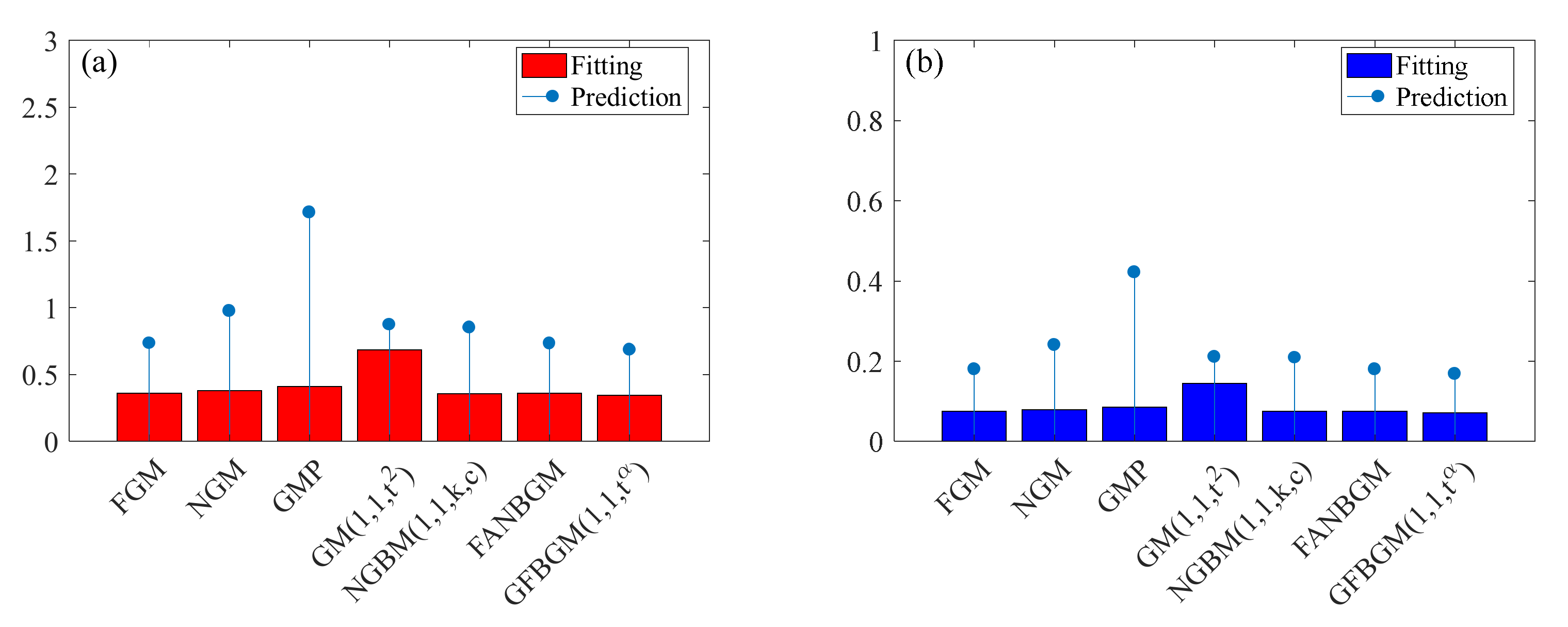
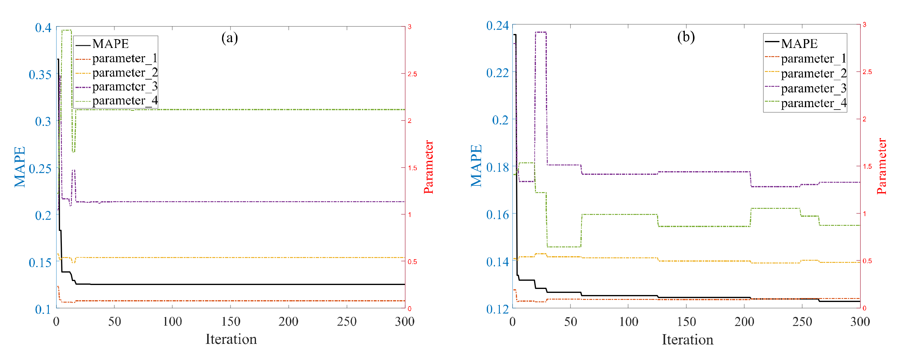
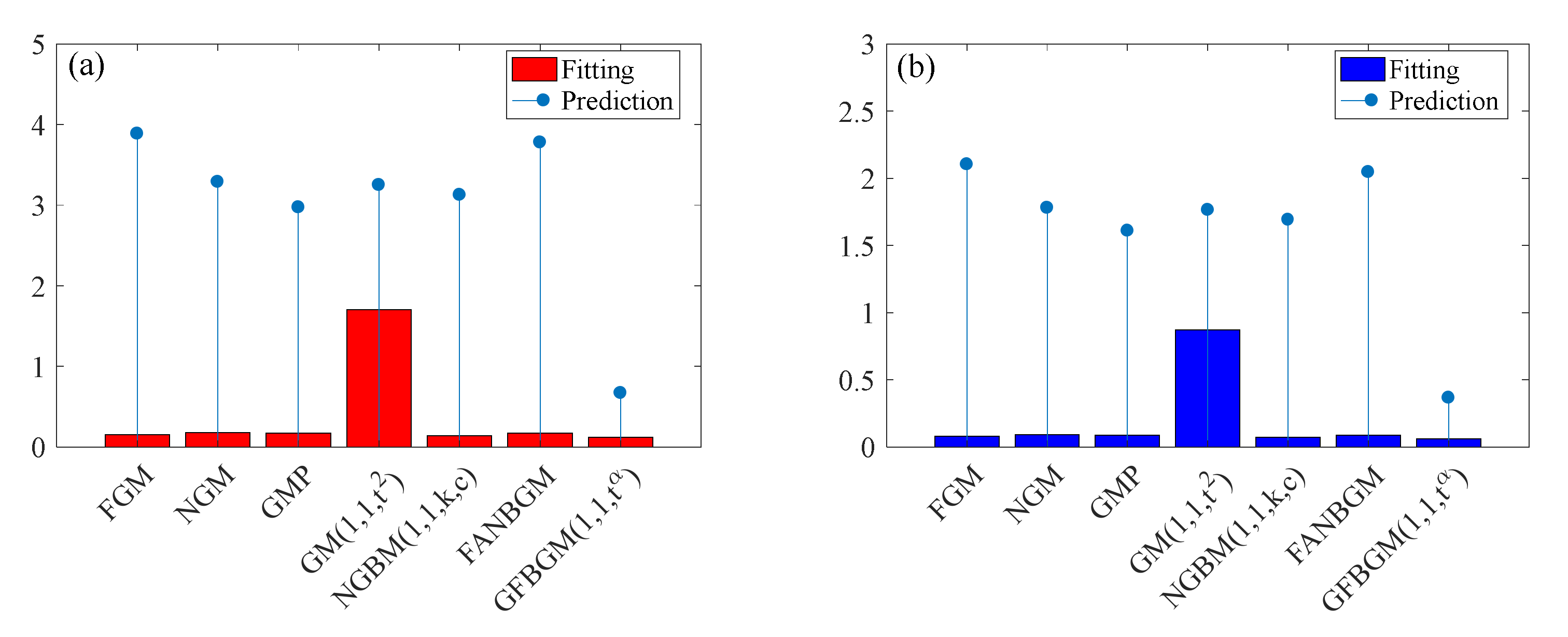
According to the Statistics Review of World Energy 2020 [4], the PPEC of India increased rapidly from 2009 to 2019. This is mainly because, in recent years, the gross domestic product (GDP) growth of India has been maintained at a high level, so the demand for primary energy has remained high. Therefore, this section takes India as a case to assess the forecasting performance of the GFGBM (1,1, t α ). The parameters and MAPEs of the GFGBM (1,1, t α ) computed by the MFO and GWO optimization algorithms are shown in Table 3. The fitting error obtained by the MFO optimization algorithm is small, but the prediction error is large, and the model exhibits overfitting. The MAPE and MAPEtest values obtained by the GWO algorithm are 0.3441% and 0.6849%, respectively, so the GWO algorithm is selected to solve the parameters. Then, the structural parameters of the GFGBM (1,1, t α ) can be obtained according to Equation (23): a = 0.1618 , b = 31.7284 , c 0 = 32.2997 . Figure 2 shows the number of iterations of the two optimization algorithms and the relationships between the MAPEs and parameters. The simulation and prediction results of the seven models are presented in Figure 3 and Table 4. The error metrics are presented in Figure 4 and Table 5. It can be seen that the MAPE values of simulation and prediction of the GFGBM (1,1, t α ) are 0.3441% and 0.6849%, respectively, and the MAE values are 0.0717 and 0.1686, respectively. The error metrics are lower than those of the other six models, which means that the proposed model has the best prediction performance. This also shows that the GFGBM (1,1, t α ) can better simulate and predict the trend of the PPEC in India.

3.1.2. PPEC of the World

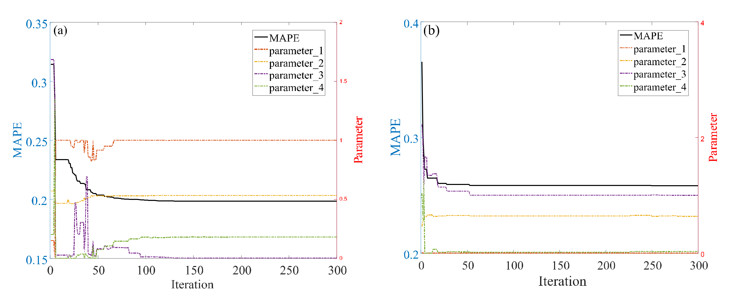
According to the Statistics Review of World Energy 2020 [4], the global PPEC fluctuated slightly from 2009 to 2019. Therefore, this section takes the global PPEC as a case to assess the forecasting performance of the GFGBM (1,1, t α ). The parameters and MAPE values of the GFGBM (1,1, t α ) computed by the MFO and GWO optimization algorithms are shown in Table 6. The MAPE and MAPEtest values of the MFO algorithm are 0.135% and 0.5997%, respectively, which are better than those of the GWO algorithm. Therefore, the MFO algorithm is used to obtain the model parameters. Then, the structural parameters of the GFGBM (1,1, t α ) can be obtained according to Equation (23): a = 1.5553 , b = 2.8476 × 10 4 , c 0 = 2.1348 × 10 5 . Figure 5 shows the number of iterations of the two optimization algorithms and the relationships between the MAPEs and parameters. The simulation and prediction results of the seven models are presented in Figure 6 and Table 7. The error metrics are presented in Figure 7 and Table 8. It can be seen that the MAPE values of simulation and prediction of the GFGBM (1,1, t α ) are 0.135% and 0.5997%, respectively, and the MAE values are 0.0996 and 0.4517, respectively. The error metrics are lower than those of the other six models, which means that the proposed model has the best prediction performance. This also shows that the GFGBM (1,1, t α ) can better simulate and predict the trend of the global PPEC.

3.1.3. PPEC of OECD Countries

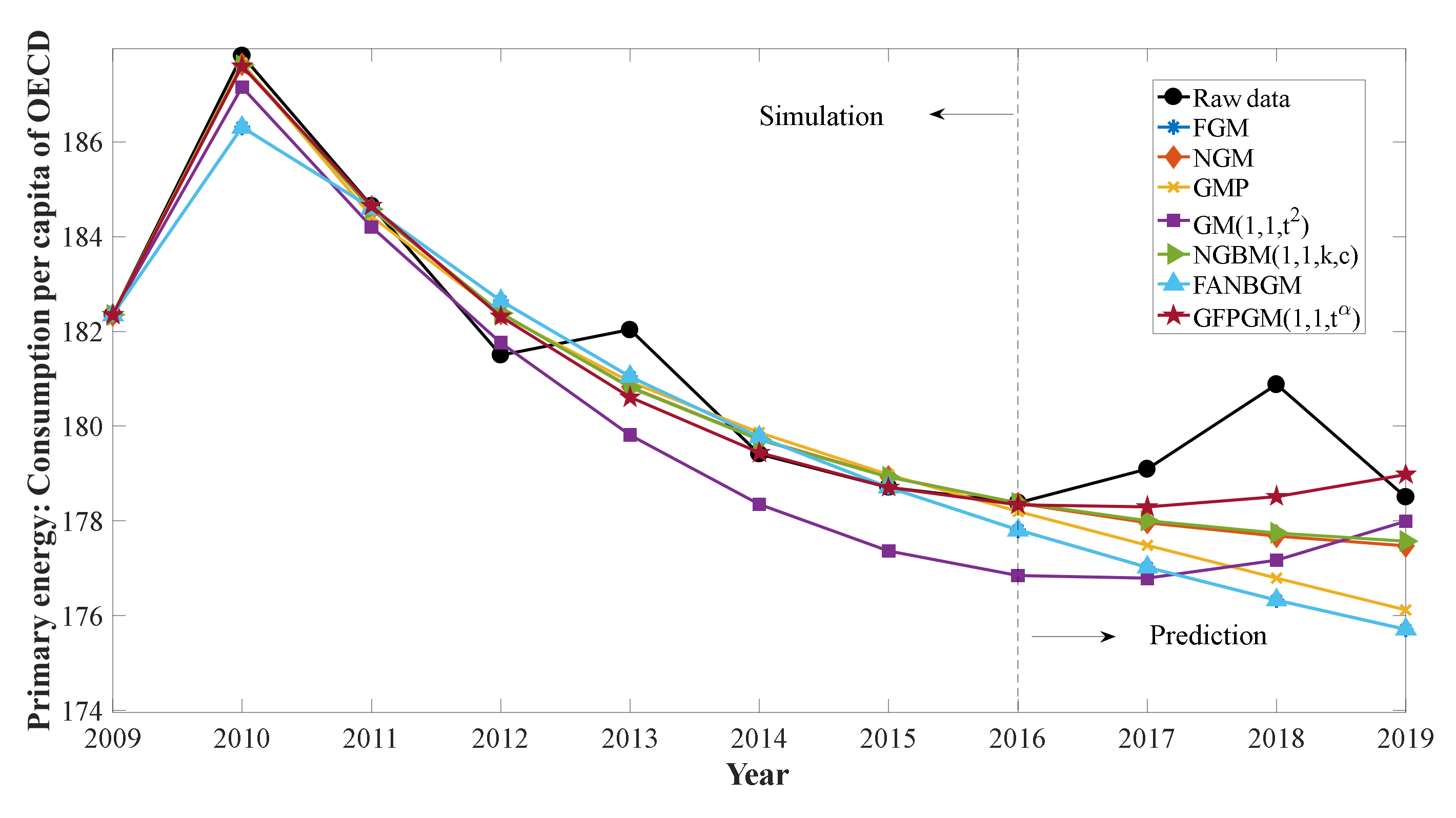
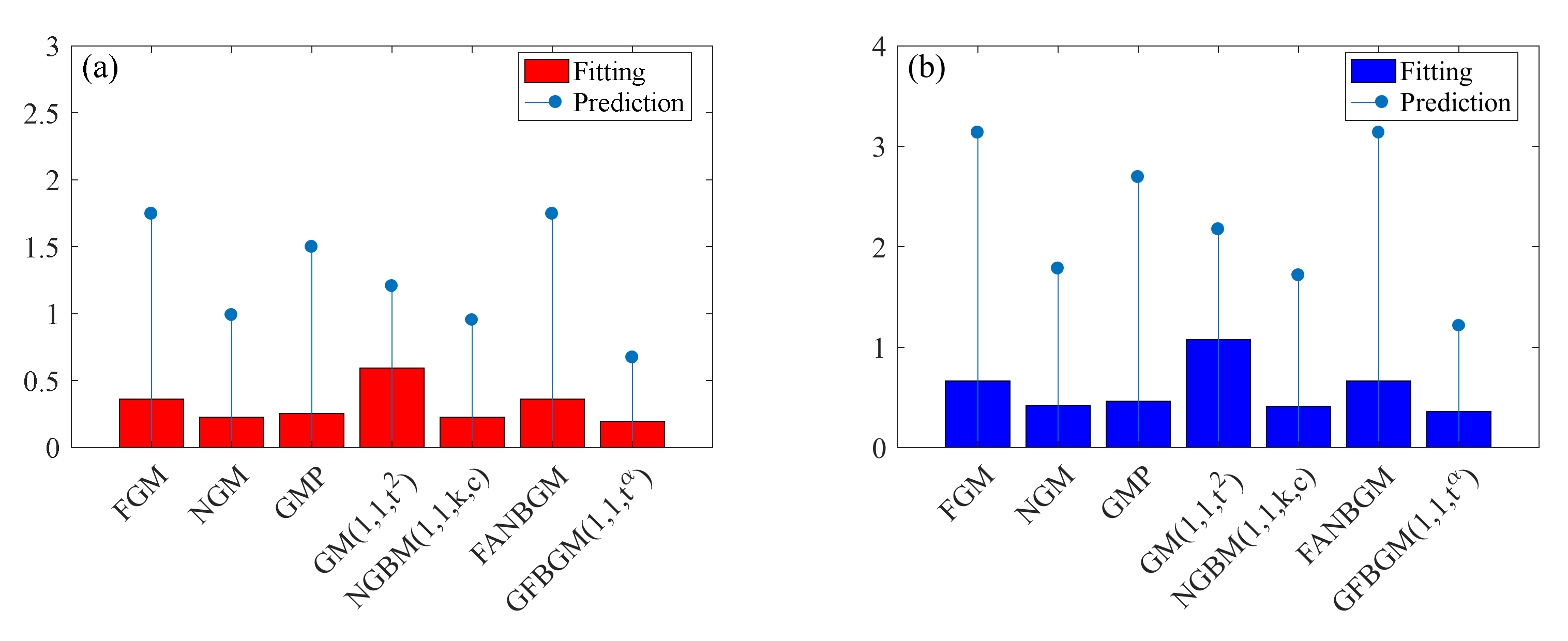
According to the Statistics Review of World Energy 2020 [4], the PPEC of the OECD fluctuated slightly from 2009 to 2019. However, the OECD countries still consist of the economies with the largest PPEC in the world. Therefore, this section takes the PPEC of the OECD countries as examples to assess the forecasting performance of the GFGBM (1,1, t α ). The parameters and MAPE values of the GFGBM (1,1, t α ) computed by the MFO and GWO optimization algorithms are shown in Table 9. The MAPE and MAPEtest of the MFO algorithm are 0.1983% and 0.6735%, respectively, which are better than those of the GWO algorithm. Therefore, the MFO algorithm is used to obtain the model parameters. Then, the structural parameters of the GFGBM (1,1, t α ) can be obtained according to Equation (23): a = 0.0201 , b = 7297.2578 , c 0 = 7237.8325 . Figure 8 shows the number of iterations of the two optimization algorithms and the relationships between the MAPEs and parameters. The simulation and prediction results of the seven models are presented in Figure 9 and Table 10. The error metrics are presented in Figure 10 and Table 11. It can be seen that the MAPE values of simulation and prediction of the GFGBM (1,1, t α ) are 0.1983% and 0.6735%, respectively, and the MAE values are 0.3614 and 1.2134, respectively. The error metrics are lower than those of the other six models, which means that the proposed model has the best prediction performance. This also shows that the GFGBM (1,1, t α ) can better simulate and predict the trend of the PPEC of OECD countries.

3.1.4. PPEC of Non-OECD

According to the Statistics Review of World Energy 2020 [4], the PPEC of non-OECD countries increased rapidly from 2009 to 2019. The developing countries, represented by China, India, and Russia, are still the countries with the largest primary energy consumption levels in the world. With rapid economic development, the demand for primary energy in these countries will remain high. Therefore, this section takes the PPEC levels of non-OECD countries as examples to assess the forecasting performance of the GFGBM (1,1, t α ). The parameters and MAPE values of the GFGBM (1,1, t α ) computed by the MFO and GWO optimization algorithms are shown in Table 12. The MAPE and MAPEtest of the GWO algorithm are 0.1228% and 0.6720%, respectively, which are better than those of the MFO algorithm. Therefore, the GWO algorithm is used to obtain the model parameters. Then, the structural parameters of the model can be obtained according to Equation (23): a = 9.2800 × 10 4 , b = 0.1012 , c 0 = 0.0689 , c 1 = 0.0024 . Figure 11 shows the relationships between the number of iterations, MAPEs, and parameters. The simulation and prediction results of the seven models are presented in Figure 12 and Table 13. The error metrics are presented in Figure 13 and Table 14. It can be seen that the MAPE values of simulation and prediction of the GFGBM (1,1, t α ) are 0.1228% and 0.6720%, respectively, and the MAE values are 0.0627 and 0.3662, respectively. The error metrics are lower than those of the other six models, which means that the proposed model has the best prediction performance. This also shows that the GFGBM (1,1, t α ) can better simulate and predict the trend of the PPEC of non-OECD countries.

3.2. Forecasting the PPEC over the Next 5 Years

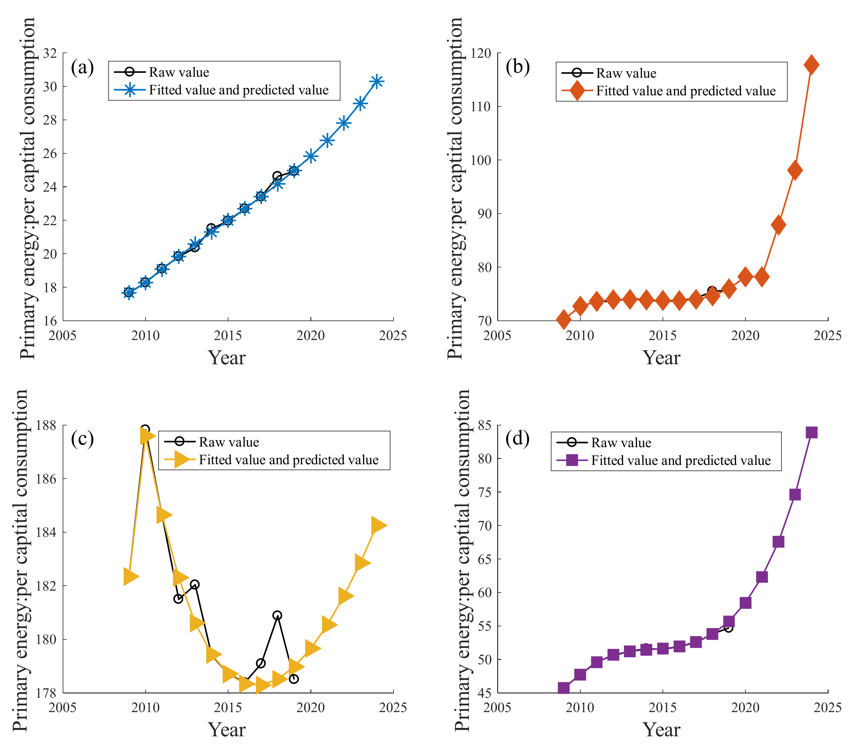
In this section, we use the GFGBM (1,1, t α ) to forecast the PPEC of India, the world, OECD countries, and non-OECD countries over the next 5 years (2020–2024). The prediction results are presented in Table 15 and Figure 14. The forecasting results indicate that the PPEC of India, the world, the OECD countries, and the non-OECD countries will increase to a certain extent over the next 5 years. Notably, the PPEC of India is expected to increase by 5.36 GJ, an increase of 51.53%; the PPEC of the world is expected to increase by 42.09 GJ, an increase of 55.61%; the PPEC of the OECD countries is expected to increase by 5.75 GJ, an increase of 3.22%; the PPEC of the non-OECD countries is expected to increase by 29.22 GJ, an increase of 53.41%. India’s economy has been growing steadily in the past decade, and its energy demand is increasing day by day. It can be predicted that the PPEC will gradually increase over the next 5 years. The global PPEC will grow rapidly, and most of the growth comes from non-OECD countries. This is because non-OECD includes many emerging economies whose economies are in the stage of rapid development. The demand for primary energy remains high, but the utilization of renewable energy is insufficient. OECD countries have better green and clean energy alternatives and financial support, which can prevent the sharp rise of PPEC. In the past ten years, the overall trend of PPEC is downward, and the volatility has occasionally increased. The prediction results show that it will grow slowly over the next 5 years, which is within the reasonable prediction range.

4. Conclusions

To more accurately predict the future PPEC of India, the world, OECD countries, and non-OECD countries, we propose a new gray model (GFGBM (1,1, t α )) based on the NGBM (1,1) and FPGM (1,1, t α ) and use the numerical integration method to obtain exact solutions for the model. At the same time, the MFO and GWO optimization algorithms are used to solve the parameters. Through parameter changes, the GFGBM (1,1, t α ) can be transformed into other gray models, so the new model has strong adaptability. The results of data fitting and forecasting for the four types of tested economies show that the error metrics of the GFGBM (1,1, t α ) are lower than those of the existing FGM, NGM, GMP (1,1,2), GM (1,1, t 2 ), NGBM (1,1,k,c), and FANGBM, which means that the GFGBM (1,1, t α ) has the best prediction performance. The proposed model can be used for the prediction of other data due to its high adaptability.
Furthermore, we use the GFGBM (1,1, t α ) to predict the PPEC of India, the world, OECD countries, and non-OECD countries over the next 5 years. The forecasting results show that from 2020 to 2024, the PPEC of all these regions will gradually rise. Notably, the PPEC of India is expected to increase by 5.36 GJ, an increase of 51.53%; the PPEC of the world is expected to increase by 42.09 GJ, an increase of 55.61%; the PPEC of the OECD countries is expected to increase by 5.75 GJ, an increase of 3.22%; the PPEC of the non-OECD countries is expected to increase by 29.22 GJ, an increase of 53.41%.
According to the prediction results of this paper, the growth rate of PPEC in the world will still be high over the next 5 years, especially in the new economy represented by India. This will inevitably lead to the continuous increase of global carbon emissions, which is contrary to the carbon emission reduction required in the SDG. Therefore, governments all over the world, especially those countries with large primary energy consumption, should attach great importance to the rapid growth of primary energy consumption. The governments should vigorously develop clean and green energy and reduce the proportion of primary energy consumption. The governments should encourage enterprises to reduce fossil energy consumption and increase the proportion of new energy consumption through environmental regulation, financial subsidies, taxation, and other measures, to gradually optimize the energy consumption structure and achieve the SDG.
Some suggestions are provided for future research. First, the existing reverse fractional-order accumulation and subtraction methods can be improved to better reflect the priority of new information. Second, a new method can be found to calculate the area of the curve trapezoid, so as to further optimize the background value to reduce the error of the gray prediction model. Third, artificial neural networks, support vector machines, and other models can be combined with GFGBM (1,1, t α ) to build a more accurate prediction model. Fourth, other optimization algorithms can be used to solve the parameters of the model.

Author Contributions

Conceptualization, H.W. and Y.W.; software Y.W.; validation, H.W.; data curation, Y.W.; writing—original draft, Y.W.; writing—review and editing, H.W.; supervision, H.W. All authors have read and agreed to the published version of the manuscript.

Funding

This work was supported by the Social Science Project of Shaanxi (No.2021D062), the Youth Innovation Team of Shaanxi Universities (No. 21JP044), and the Scientific Research Project of China (Xi’an) Institute for Silk Road Research (No. 2019YA08).

Institutional Review Board Statement

Not applicable.

Informed Consent Statement

Not applicable.

Data Availability Statement

The datasets of this paper are available from the corresponding author on reasonable request.

Conflicts of Interest

The authors declare no conflict of interest.

Nomenclature

PPECPer capita primary energy consumption
FOAFractional order (r-order) accumulation
IFOAInverse fractional order (r-order) accumulation
X ( 0 ) Original series
X ( 1 ) First-order accumulated series
GM (1,1)Basic gray model
FGM (1,1)Fractional gray model
NGM (1,1)Nonlinear gray model
GMP (1,1,2)Gray model with polynomial term
GM (1,1, t α )Gray model with time power
NGBM (1,1)Nonlinear gray Bernoulli model
FANGBM (1,1)Fractional nonlinear gray Bernoulli model
FPGM(1,1, t α )Fractional gray polynomial model with time power term
GFGBM (1,1, t α )Fractional gray Bernoulli model with time power term
GWOGray wolf optimization
MFOMoth flame optimization
MAPEMean absolute percentage error
MAEMean absolute percentage error

References

  1. Ceglia, F.; Macaluso, A.; Marrasso, E.; Roselli, C.; Vanoli, L. Energy, Environmental, and Economic Analyses of Geothermal Polygeneration System Using Dynamic Simulations. Energies 2020, 13, 4603. [Google Scholar] [CrossRef]
  2. Ceglia, F.; Marrasso, E.; Roselli, C.; Sasso, M. An innovative environmental parameter: Expanded total equivalent warming impact. Int. J. Refrig. 2021, 131, 980–989. [Google Scholar] [CrossRef]
  3. Cellura, M.; Fichera, A.; Guarino, F.; Volpe, R. Sustainable development goals and performance measurement of positive energy district: A methodological approach. In Sustainability in Energy and Buildings; Springer: Singapore, 2021; pp. 519–527. [Google Scholar]
  4. British Petroleum. BP Statistical Review of World Energy. Available online: https://www.bp.com/ (accessed on 11 October 2021).
  5. Merino, I.; Herrera, I.; Valdés, H. Environmental assessment of energy scenarios for a low-carbon electrical network in Chile. Sustainability 2019, 11, 5066. [Google Scholar] [CrossRef] [Green Version]
  6. Chen, H.; He, L.; Chen, J.; Yuan, B.; Huang, T.; Cui, Q. Impacts of clean energy substitution for polluting fossil-fuels in terminal energy consumption on the economy and environment in China. Sustainability 2019, 11, 6419. [Google Scholar] [CrossRef] [Green Version]
  7. Shen, N.; Wang, Y.; Peng, H.; Hou, Z. Renewable energy green innovation, fossil energy consumption, and air pollution: Spatial empirical analysis based on China. Sustainability 2020, 12, 6397. [Google Scholar] [CrossRef]
  8. Li, Z.; Li, Y.B.; Shao, S.S. Analysis of influencing factors and trend forecast of carbon emission from energy consumption in China based on expanded STIRPAT model. Energies 2019, 12, 3054. [Google Scholar] [CrossRef] [Green Version]
  9. Harsh, P.; Manan, S. Energy consumption and price forecasting through data-driven analysis methods: A review. SN Comput. Sci. 2021, 2, 315. [Google Scholar]
  10. Kongbuamai, N.; Bui, Q.; Nimsai, S. The effects of renewable and nonrenewable energy consumption on the ecological footprint: The role of environmental policy in BRICS countries. Environ. Sci. Pollut. Res. 2021, 28, 27885–27899. [Google Scholar] [CrossRef]
  11. Sen, P.; Roy, M.; Pal, P. Application of ARIMA for forecasting energy consumption and GHG emission: A case study of an Indian pig iron manufacturing organization. Energy 2016, 116, 1031–1038. [Google Scholar] [CrossRef]
  12. Bianco, V.; Manca, O.; Nardini, S. Electricity consumption forecasting in Italy using linear regression models. Energy 2009, 34, 1413–1421. [Google Scholar] [CrossRef]
  13. Zhang, K.; Feng, W.B. Prediction of China’s total energy consumption based on bayesian arima-nonlinear regression model. In IOP Conference Series: Earth and Environmental Science; IOP Publishing: Bristol, UK, 2021; Volume 657, p. 012056. [Google Scholar]
  14. Nawaz, S.; Iqbal, N.; Anwar, S. Modelling electricity demand using the STAR (smooth transition auto-regressive) model in Pakistan. Energy 2014, 78, 535–542. [Google Scholar] [CrossRef]
  15. Cheong, C.W. Parametric and non-parametric approaches in evaluating martingale hypothesis of energy spot markets. Math. Comput. Model. 2011, 54, 1499–1509. [Google Scholar] [CrossRef]
  16. Karimi, H.; Dastranj, J. Artificial neural network-based genetic algorithm to predict natural gas con sumption. Energy Syst. 2014, 5, 571–581. [Google Scholar] [CrossRef]
  17. Ahmad, M.W.; Mourshed, M.; Rezgui, Y. Trees vs Neurons: Comparison between random forest and ANN for high-resolution prediction of building energy consumption. Energy Build. 2017, 147, 77–89. [Google Scholar] [CrossRef]
  18. Touzani, S.; Granderson, J.; Fernandes, S. Gradient boosting machine for modeling the energy consumption of commercial buildings. Energy Build. 2018, 158, 1533–1543. [Google Scholar] [CrossRef] [Green Version]
  19. Wang, X.; Luo, D.; Zhao, X.; Sun, Z. Estimates of energy consumption in China using a self-adaptive multi-verse optimizer-based support vector machine with rolling cross-validation. Energy 2018, 152, 539–548. [Google Scholar] [CrossRef]
  20. Kim, C.H.; Kim, M.; Song, Y.J. Sequence-to-sequence deep learning model for building energy consumption prediction with dynamic simulation modeling. J. Build. Eng. 2021, 43, 102577. [Google Scholar] [CrossRef]
  21. Lee, Y.S.; Tong, L.I. Forecasting energy consumption using a Grey model improved by incorporating genetic programming. Energy Convers. Manag. 2011, 52, 147–152. [Google Scholar] [CrossRef]
  22. Deng, J. Control problems of grey systems. Syst. Control Lett. 1982, 1, 288–294. [Google Scholar]
  23. Ma, X.J.; Jiang, P.; Jiang, Q.C. Research and application of association rule algorithm and an optimized grey model in carbon emissions forecasting. Technol. Forecast. Soc. Change 2020, 158, 120159. [Google Scholar] [CrossRef]
  24. Tong, Y.; Yan, Z.; Chao, L. Research on a grey prediction model of population growth based on a logistic approach. Discret. Dyn. Nat. Soc. 2020, 2020, 2416840. [Google Scholar] [CrossRef]
  25. Wang, Z.X.; Jv, Y.Q. A non-linear systematic grey model for forecasting the industrial economy-energy-environment system. Technol. Forecast. Soc. Change 2021, 167, 120707. [Google Scholar] [CrossRef]
  26. Liu, C.; Xie, W.L.; Wu, W.Z.; Zhu, H.G. Predicting Chinese total retail sales of consumer goods by employing an extended discrete grey polynomial model. Eng. Appl. Artif. Intell. 2021, 102, 104261. [Google Scholar] [CrossRef]
  27. Xie, W.L.; Wu, W.Z.; Liu, C.; Zhang, T.; Dong, Z.J. Forecasting fuel combustion-related CO2 emissions by a novel continuous fractional nonlinear grey Bernoulli model with grey wolf optimizer. Environ. Sci. Pollut. Res. 2021, 28, 38128–38144. [Google Scholar] [CrossRef]
  28. Wu, W.Q.; Ma, X.; Zeng, B.; Wang, Y.; Cai, W. Application of the novel fractional grey model FAGMO(1,1,k) to predict China’s nuclear energy consumption. Energy 2018, 165, 223–234. [Google Scholar] [CrossRef] [Green Version]
  29. Ding, S.; Hipel, K.W.; Dang, Y.G. Forecasting China’s electricity consumption using a new grey prediction model. Energy 2018, 149, 314–328. [Google Scholar] [CrossRef]
  30. Wu, W.Q.; Ma, X.; Zeng, B.; Wang, Y.; Cai, W. Forecasting short-term renewable energy consumption of China using a novel fractional nonlinear grey Bernoulli model. Renew. Energy 2019, 140, 70–87. [Google Scholar] [CrossRef]
  31. Liu, C.; Wu, W.Z.; Xie, W.L.; Zhang, J. Application of a novel fractional grey prediction model with time power term to predict the electricity consumption of India and China. Chaos Soliton. Fract. 2020, 141, 110429. [Google Scholar] [CrossRef]
  32. Liu, C.; Wu, W.Z.; Xie, W.L.; Zhang, T.; Zhang, J. Forecasting natural gas consumption of China by using a novel fractional grey model with time power term. Energy Rep. 2021, 7, 788–797. [Google Scholar] [CrossRef]
  33. Wu, W.Z.; Pang, H.D.; Zheng, C.L.; Xie, W.L.; Liu, C. Predictive analysis of quarterly electricity consumption via a novel seasonal fractional nonhomogeneous discrete grey model: A case of Hubei in China. Energy 2021, 229, 120714. [Google Scholar] [CrossRef]
  34. Zeng, L. Forecasting the primary energy consumption using a time delay grey model with fractional order accumulation. Math. Comp. Model. Dyn. Syst. 2021, 27, 31–49. [Google Scholar] [CrossRef]
  35. Cui, J.; Liu, S.F.; Zeng, B.; Xie, N.M. A novel grey forecasting model and its optimization. Appl. Math. Model. 2013, 37, 4399–4406. [Google Scholar] [CrossRef]
  36. Chen, P.Y.; Yu, H.M. Foundation settlement prediction based on a novel NGM model. Math. Probl. Eng. 2014, 2014, 242809. [Google Scholar] [CrossRef]
  37. Qian, W.Y.; Dang, Y.G.; Liu, S.F. Grey GM(1,1,) model with time power and its application. Syst. Eng. Theory Pract. 2012, 32, 2247–2252. [Google Scholar]
  38. Luo, D.; Wei, B. Grey forecasting model with polynomial term and its optimization. J. Grey Syst. 2017, 29, 58–69. [Google Scholar]
  39. Ma, X.; Liu, Z.B. Application of a novel time-delayed polynomial grey model to predict the natural gas consumption in China. J. Comput. Appl. Math. 2017, 324, 17–24. [Google Scholar] [CrossRef]
  40. Chen, C.I. Application of the novel nonlinear grey Bernoulli model for forecasting unemployment rate. Chaos Soliton. Fract. 2008, 37, 278–287. [Google Scholar] [CrossRef]
  41. Şahin, U. Projections of Turkey’s electricity generation and installed capacity from total renewable and hydro energy using fractional nonlinear grey Bernoulli model and its reduced forms. Sustain. Prod. Consump. 2020, 23, 52–62. [Google Scholar] [CrossRef]
  42. Jiang, J.; Wu, W.Z.; Li, Q.; Zhang, Y. A PSO algorithm-based seasonal nonlinear grey Bernoulli model with fractional order accumulation for forecasting quarterly hydropower generation. J. Intell. Fuzzy Syst. 2021, 40, 507–519. [Google Scholar] [CrossRef]
  43. Ma, X.; Liu, Z. The GMC(1, n) model with optimized parameters and its applications. J. Grey Syst. 2017, 29, 121–137. [Google Scholar]
  44. Liu, X.; Xie, N.M. A nonlinear grey forecasting model with double shape parameters and its application. Appl. Math. Comput. 2019, 360, 203–212. [Google Scholar] [CrossRef]
  45. Xie, W.L.; Yu, G.X.; Zargarzadeh, H. A novel conformable fractional nonlinear grey Bernoulli model and its application. Complexity 2020, 2020, 9178098. [Google Scholar] [CrossRef]
  46. Zheng, C.L.; Wu, W.Z.; Xie, W.L.; Li, Q. A MFO-based conformable fractional nonhomogeneous grey Bernoulli model for natural gas production and consumption forecasting. Appl. Soft Comput. 2020, 99, 106891. [Google Scholar] [CrossRef]
  47. Wu, W.Q.; Ma, X.; Zeng, B.; Lv, W.Y. A novel grey Bernoulli model for short-term natural gas consumption forecasting. Appl. Math. Model. 2020, 84, 393–404. [Google Scholar] [CrossRef]
  48. Xiao, Q.Z.; Gao, M.Y.; Xiao, X.P.; Goh, M. A novel grey Riccati-Bernoulli model and its application for the clean energy consumption prediction. Eng. Appl. Artif. Intell. 2020, 95, 103863. [Google Scholar] [CrossRef]
  49. Xu, K.; Pang, X.Y.; Duan, H.M. An optimization grey Bernoulli model and its application in forecasting oil consumption. Math. Probl. Eng. 2021, 2021, 5598709. [Google Scholar] [CrossRef]
  50. Mirjalili, S. Moth-flame optimization algorithm: A novel nature-inspired heuristic paradigm. Knowl.-Based Syst. 2015, 89, 228–249. [Google Scholar] [CrossRef]
  51. Wu, L.F.; Liu, S.F.; Yao, L.G.; Yan, S.L.; Liu, D.L. Grey system model with the fractional order accumulation. Commun. Nonlinear Sci. Numer. Simul. 2013, 18, 1775–1785. [Google Scholar] [CrossRef]
  52. Cui, J.; Dang, Y.; Liu, S. Novel gray forecasting model and its modeling mechanism. Control Decis. 2009, 24, 1702–1706. [Google Scholar]
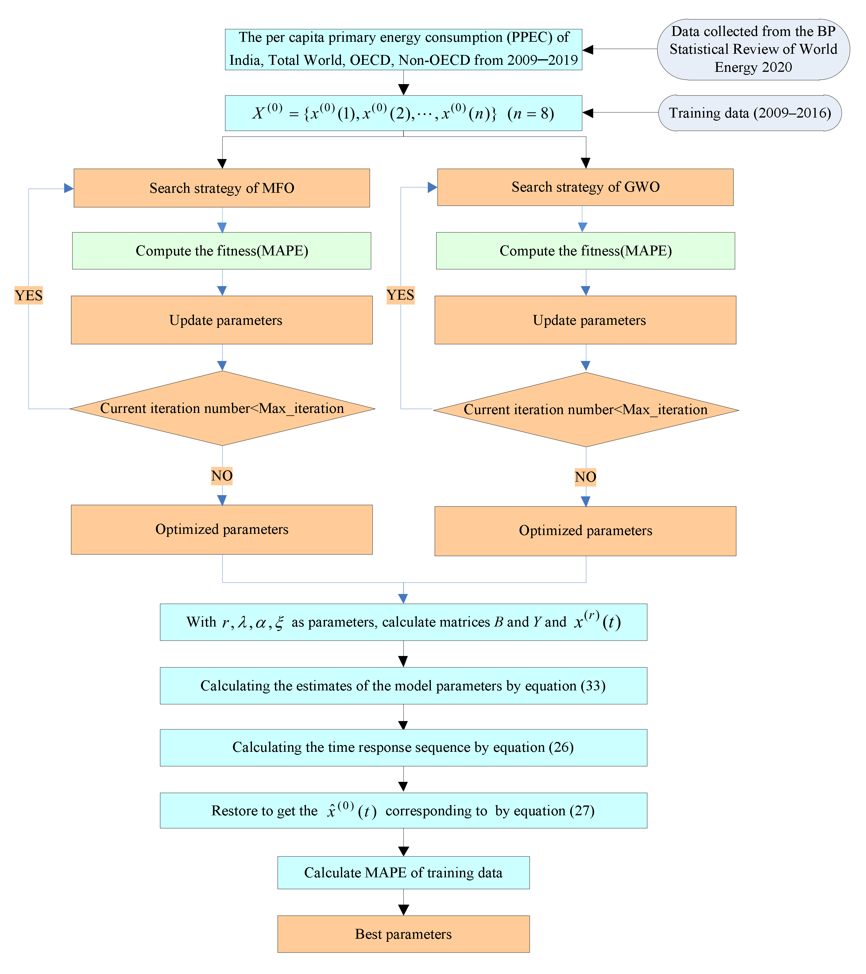
Figure 1. Algorithm implementation process of GFGBM (1,1, t α ).
Sustainability 14 02431 g001
Figure 2. Iterations, MAPE, and parameters of the two optimization algorithms (a): MFO; (b): GWO.
Sustainability 14 02431 g002
Figure 3. Results of PPEC in India.
Sustainability 14 02431 g003
Figure 4. Error metrics of PPEC in India (a): MAPE; (b): MAE.
Sustainability 14 02431 g004
Figure 5. Iterations, MAPE, and parameters of the two optimization algorithms: (a): MFO; (b): GWO.
Sustainability 14 02431 g005
Figure 6. Results of PPEC in the total world.
Sustainability 14 02431 g006
Figure 7. Error metrics of PPEC in the total world (a): MAPE; (b): MAE.
Sustainability 14 02431 g007
Figure 8. Iterations, MAPE, and parameters of the two optimization algorithms (a): MFO; (b): GWO.
Sustainability 14 02431 g008
Figure 9. Results of PPEC in OECD.
Sustainability 14 02431 g009
Figure 10. Error metrics of PPEC in OECD (a): MAPE; (b): MAE.
Sustainability 14 02431 g010
Figure 11. Iterations, MAPE, and parameters of the two optimization algorithms (a): MFO; (b): GWO.
Sustainability 14 02431 g011
Figure 12. Results of PPEC in non-OECD.
Sustainability 14 02431 g012
Figure 13. Error metrics of PPEC in non-OECD (a): MAPE; (b): MAE.
Sustainability 14 02431 g013
Figure 14. Predictions for the PPEC over the next 5 years of the (a): India; (b): The word; (c): OECD; (d): Non-OECD.
Sustainability 14 02431 g014
Table 1. PPEC of the four types of economies (GJ) (Adapted from ref. [4]).
YearIndiaTotal WorldOECDNon-OECD
200917.675970.2346182.346945.7504
201018.273672.7214187.819547.7449
201119.100073.5948184.648949.6531
201219.840373.6576181.499250.5636
201320.359274.1683182.033551.2263
201421.504873.9022179.408451.6154
201521.959973.5879178.707351.5342
201622.700773.7523178.382051.9503
201723.407174.2340179.091952.5323
201824.619875.4954180.878653.8343
201924.926175.6834178.504954.6977
Table 2. Error metric.
NameAbbreviationFormulation
Mean absolute percentage errorMAPE 1 n 1 k = 2 n | x ( 0 ) ( k ) x ^ ( 0 ) ( k ) x ( 0 ) ( k ) | × 100 %
Mean absolute errorMAE 1 n 1 k = 2 n | x ^ ( 0 ) ( k ) x ( 0 ) ( k ) |
Table 3. Parameters and MAPEs of the GFGBM (1,1, t α ) based on different optimization algorithms (Case 1).
Algorithmr
(Parameter 1)
λ
(Parameter 2)
α
(Parameter 3)
ξ
(Parameter 4)
MAPE (%)MAPEtest (%)
MFO0.63520.51620.00020.00000.32580.9084
GWO0.07830.51510.01800.20490.34410.6849
Table 4. Simulation results and prediction results of PPEC in India.
YearDataFGMNGMGMPGM (1,1, t 2 )NGBM (1,1,k,c)FANGBMGFGBM
200917.675917.675917.675917.675917.675917.675917.675917.6759
201018.273618.273618.285618.268818.323718.246718.273418.2737
201119.100019.078519.059419.034719.124319.094219.078519.0712
201219.840319.825019.818619.790319.913119.840319.825119.8443
201320.359220.550720.563420.533220.689620.554620.550820.5816
201421.504821.271821.294121.260121.453021.265121.271921.2942
201521.959921.996722.010921.967122.202821.986621.996721.9958
201622.700722.730322.714222.649222.938322.728822.730222.7003
YeardataFGMNGMGMP GM (1,1, t 2 )NGBM (1,1,k,c)FANGBMGFGBM
201723.407123.476223.404223.300223.658723.498623.475923.4215
201824.619824.236624.081023.912324.363424.301724.236324.1735
201924.926125.013624.745124.475925.051625.142925.013124.9711
Table 5. Error metrics of PPEC in India.
SimulationFGMNGMGMPGM (1,1, t 2 )NGBM (1,1,k,c)FANGBMGFGBM
MAPE (%)0.35880.38030.41030.68350.35680.35880.3441
MAE0.07540.07910.08540.14430.07470.07540.0717
PredictionFGMNGMGMP GM (1,1, t 2 )NGBM (1,1,k,c)FANGBMGFGBM
MAPE (%)0.73420.97571.71220.87330.85090.73350.6849
MAE0.17990.24090.42150.21120.20880.17980.1686
Table 6. Parameters and MAPEs of the GFGBM (1,1, t α ) based on different optimization algorithms (Case 2).
Algorithmr
(Parameter 1)
λ
(Parameter 2)
α
(Parameter 3)
ξ
(Parameter 4)
MAPE (%)MAPEtest (%)
MFO0.04590.59033.00003.00000.13500.5997
GWO0.00000.59760.99930.00460.15032.1902
Table 7. Simulation results and prediction results of PPEC in the total world.
YearDataFGMNGMGMPGM (1,1, t 2 )NGBM (1,1,k,c)FANGBMGFGBM
200970.234670.234670.234670.234670.234670.234670.234670.2346
201072.721472.721472.846672.774372.998572.721472.580772.7214
201173.594873.512773.539273.522473.612273.539773.469873.6288
201273.657673.849873.755173.842974.065973.844873.770673.9435
201374.168373.957373.822473.929974.357673.925273.844473.9909
201473.902273.926373.843473.889374.485173.889273.834773.8971
201573.587973.803073.849973.779274.446273.788873.797073.7761
201673.752373.614373.852073.631074.238973.652573.752373.7587
YearDataFGMNGMGMP GM (1,1, t 2 )NGBM (1,1,k,c)FANGBMGFGBM
201774.234073.376973.852673.462073.860973.497273.708273.9941
201875.495473.102373.852873.281773.310073.333673.667074.6553
201975.683472.798373.852973.095272.583973.168373.629175.9585
Table 8. Error metrics of PPEC in the total world.
SimulationFGMNGMGMPGM (1,1, t 2 )NGBM (1,1,k,c)FANGBMGFGBM
MAPE (%)0.16700.20250.16940.54700.15470.18980.1350
MAE0.12320.14920.12490.40280.11420.13990.0996
PredictionFGMNGMGMP GM (1,1, t 2 )NGBM (1,1,k,c)FANGBMGFGBM
MAPE (%)2.71221.70272.46402.49762.39311.94820.5997
MAE2.04511.28481.85801.88601.80461.46950.4517
Table 9. Parameters and MAPEs of the GFGBM (1,1, t α ) based on different optimization algorithms (Case 3).
Algorithmr
(Parameter 1)
λ
(Parameter 2)
α
(Parameter 3)
ξ
(Parameter 4)
MAPE (%)MAPEtest (%)
MFO1.00000.53250.00180.17970.19830.6735
GWO0.00040.63811.00040.03000.25820.6132
Table 10. Simulation results and prediction results of PPEC in OECD.
YearDataFGMNGMGMPGM (1,1, t 2 )NGBM (1,1,k,c)FANGBMGFGBM
2009182.3469182.3469182.3469182.3469182.3469182.3469182.3469182.3469
2010187.8195186.3057187.6371187.6585187.1542187.6202186.3057187.5961
2011184.6489184.5967184.5695184.4182184.2045184.5846184.5967184.6489
2012181.4992182.6416182.3844182.3552181.7614182.3867182.6416182.3105
2013182.0335181.0489180.8279180.9338179.8145180.8185181.0489180.6097
2014179.4084179.7673179.7191179.8620178.3535179.7081179.7673179.4396
2015178.7073178.7073178.9293178.9809177.3686178.9271178.7073178.7073
2016178.3820177.8061178.3667178.2036176.8499178.3820177.8061178.3421
YearDataFGMNGMGMP GM (1,1, t 2 )NGBM (1,1,k,c)FANGBMGFGBM
2017179.0919177.0231177.9659177.4829176.7879178.0051177.0230178.2911
2018180.8786176.3312177.6804176.7930177.1731177.7478176.3312178.5140
2019178.5049175.7117177.4771176.1200177.9965177.5754175.7117178.9798
Table 11. Error metrics of PPEC in OECD.
SimulationFGMNGMGMPGM (1,1, t 2 )NGBM (1,1,k,c)FANGBMGFGBM
MAPE (%)0.36110.22800.25600.59350.22680.36110.1983
MAE0.66110.41440.46471.07380.41220.66110.3614
PredictionFGMNGMGMP GM (1,1, t 2 )NGBM (1,1,k,c)FANGBMGFGBM
MAPE (%)1.74470.99091.49771.20660.95281.74470.6735
MAE3.13651.78402.69322.17261.71573.13651.2134
Table 12. Parameters and MAPEs of the GFGBM (1,1, t α ) based on different optimization algorithms (Case 4).
Algorithmr
(Parameter 1)
λ
(Parameter 2)
α
(Parameter 3)
ξ
(Parameter 4)
MAPE (%)MAPEtest (%)
MFO0.08030.53991.13552.11420.12530.8079
GWO0.10110.48171.32750.87170.12280.6720
Table 13. Simulation results and prediction results of PPEC in non-OECD.
YearDataFGMNGMGMPGM (1,1, t 2 )NGBM (1,1,k,c)FANGBMGFGBM
200945.750445.750445.750445.750445.750445.750445.750445.7504
201047.744947.761147.846347.845148.277147.744947.744947.7450
201149.653149.561849.605049.634249.815249.622049.430949.5993
201250.563650.604350.611950.610251.084450.606150.552850.6956
201351.226351.226351.188351.161452.072551.174151.237451.2266
201451.615451.582851.518351.490652.766551.516051.614951.4548
201551.534251.757151.707251.703953.153051.726451.784951.6244
201651.950351.799151.815351.856553.217751.858151.818051.9486
YearDataFGMNGMGMP GM (1,1, t 2 )NGBM (1,1,k,c)FANGBMGFGBM
201752.532351.741151.877351.977552.946151.942951.763152.6159
201853.834351.605551.912752.082052.322652.000651.653453.8011
201954.697751.408351.933052.177851.331052.044051.511355.6796
Table 14. Error metrics of PPEC in non-OECD.
SimulationFGMNGMGMPGM (1,1, t 2 )NGBM (1,1,k,c)FANGBMGFGBM
MAPE (%)0.15500.18040.17411.70490.14170.17610.1228
MAE0.07930.09160.08840.87120.07280.08970.0627
PredictionFGMNGMGMP GM (1,1, t 2 )NGBM (1,1,k,c)FANGBMGFGBM
MAPE (%)3.88673.29032.97273.25033.12663.78030.6720
MAE2.10311.78041.60901.76411.69232.04550.3662
Table 15. Predictions for the PPEC over the next 5 years (GJ).
YearIndiaTotal WorldOECDNon-OECD
202025.830578.2057179.664258.4434
202126.769978.2057180.548062.3191
202227.810187.8733181.615867.5903
202328.975098.0839182.855174.6253
202430.2928117.7758184.255783.9136
Publisher’s Note: MDPI stays neutral with regard to jurisdictional claims in published maps and institutional affiliations.