A Capacity Cost-Sharing Contract for a Two-Stage Supply Chain with a Risk-Averse Supplier under a Bargaining Power

Abstract

This study considers a two-stage supply chain (SC) consisting of a single supplier and a manufacturer. When the manufacturer introduces a new product to the market, both the manufacturer and supplier should install production capacity in advance. Since capacity building often takes a long time, the demand is uncertain at the time of capacity decision making. The supplier often makes a conservative decision on capacity building to avoid possible capital risks due to excess capacity, which leads to the so-called double marginalization problem. Various risk-sharing supply contracts have recently been studied in academia to overcome the double marginalization problem. However, most existing studies ignore the bargaining power of each SC member and capacity investment. This study aims to fill the research gap by including capacity investment and bargaining power in the supply contract process. A capacity cost-sharing (CCS) contract is introduced in which the manufacturer shares the supplier’s capacity investment risk. We investigate how to set the contract parameters in the CCS contract to coordinate the supply chain. It is found that the wholesale price and manufacturer’s CCS ratio are negatively proportional to each other, and the manufacturer’s expected profit increases as the CCS ratio (wholesale price) increases (decreases) in the coordinated CCS contract. We show that there exists a CCS contract leading to a coordinated supply chain for a specific range of bargaining power. We also present a new CCS contract for a supply chain with a risk-averse supplier. A numerical illustration is provided to clarify how the contract parameters are determined and to examine the effect of the contract parameters on SC performance. Managerial implications and possible future work are discussed.

1. Introduction

This paper considers a two-stage supply chain (SC) consisting of a single component supplier (‘supplier’ or ‘she’ for short hereafter) and a single OEM manufacturer (‘manufacturer’ or ‘he’ for short). The manufacturer buys components from the supplier, uses them to make final products, and sells them. When a company develops a new product and puts it on the market, it is necessary for both the manufacturer and supplier to secure capacity before the new product is released. Since it often takes a long time to build the capacity, the decision on capacity should be made in advance, usually based on forecasted demand, which is often highly uncertain. Capacity investment risk due to demand uncertainty is usually borne by the company investing the relevant capital [1]. From the supplier’s perspective, if the components that they produce are used exclusively for the product of the downstream manufacturer, the supplier may suffer from capital loss due to over-investment in capacity when actual demand is less than the forecasted demand. The modern market environment, including its capital-intensive supply chains, short product life cycles, and rapid changes in production technology, amplifies supply chain risks. Because of the SC risks, the supplier is often conservative in her capacity investment decisions, resulting in under-investment in capacity. However, such conservative investments may cause a shortfall in component supplies when the actual demand is greater than the predicted demand.

The decision making of SC stakeholders for their own goals often leads to the so-called double marginalization problem. Double marginalization refers to a phenomenon in which the decisions made by an independent SC member undermine overall supply chain efficiency, so the optimization of the entire supply chain cannot be achieved. A typical approach to resolving the double marginalization problem is vertical integration, which allows a company to streamline its operations by taking direct ownership of various production stages rather than relying on external suppliers [2]. Since a central manager is able to control all decisions, the double marginalization problem can be solved through centralized decision making. However, vertical integration has some disadvantages, including the significant capital investment required and the demand volatility risks that are undertaken alone by a single firm. Hence, it is not uncommon in industries for members within a supply chain to be independent [3,4].

A contract that ensures that the individual decisions of the SC members are aligned with the global optimum of the entire supply chain is called a channel-coordinated contract. To optimize the whole supply chain in a decentralized supply chain, sharing the risks among supply chain members is often required. There are many cases in industries where the downstream SC members share the risks to reduce the investment risk of the suppliers and improve the efficiency of the supply chain. For example, Apple invests USD 2.7 billion in display supplier LG to increase the OLED display production capacity [5]. Hyundai Motor Group and LG Energy Solution have an agreement to invest USD 1.1 billion to secure a stable supply of battery cells for their battery electric vehicles [6]. Various risk-sharing supply contracts have recently been studied in academia to achieve channel-coordinated contracts, including buy-back contracts, revenue-sharing contracts, option contracts, and so on [7,8].

The profits accrued in the supply chain are distributed among the supply chain members. The bargaining powers of the SC members affect their profit shares. When a downstream manufacturer’s bargaining power is strong, a larger portion of SC profit is taken by the manufacturer. Asymmetric dependence between the SC members is a key source of bargaining power by which one SC stakeholder can control the other to gain desirable outcomes [9]. A manufacturer’s dependence on his supplier rises if the manufacturer faces difficulty in finding alternative suppliers, resulting in more bargaining power of the supplier, and vice versa. Most existing studies on supply contracts deal with supply chains consisting of suppliers and retailers, focusing on how the supply chain is coordinated to maximize the SC profit without considering bargaining power and capacity building. Hence, the results from existing contracts may not satisfy the bargaining power constraints given in the supply chain. We attempt to fill the research gap by including capacity and bargaining power in the supply contract process. A capacity cost-sharing (CCS) contract is introduced for a two-stage supply chain in which the manufacturer shares the investment risk with the supplier. We investigate how to design the contract parameters in the CCS contract to coordinate the supply chain and examine the relationship between the contract parameters and bargaining power.

We also consider a supply chain with a risk-averse supplier. Most investment decisions aim at maximizing the expected profits. However, a supplier may consider profit variability a vital decision criterion for financial risk. The propensity of supply chain members toward risks is categorized into risk-neutral, risk-averse, and risk-seeking [10]. Risk-neutral members have a primary purpose of maximizing revenues regardless of the degree of risk. Risk-averse members tend to give up some profits to reduce risk. Risk-seeking members refer to those participants who can accept increased risk for additional profits. Companies may face a business crisis due to a single big loss even if they make profits most of the time. Hence, companies tend to take the adverse effects coming from losses more seriously than the positive effects coming from profits.

In summary, this paper attempts to answer the following questions: (1) How do we determine the capacity in a supplier–manufacturer supply chain in which both members need to build the capacity? (2) Do there exist any CCS contract parameters that lead to a coordinated supply chain given a relative bargaining power? (3) How does the bargaining power affect the contract parameters of a coordinated contract? (4) How can we design a supply contract for a supply chain with a risk-averse supplier? To answer these questions, we begin by examining how to determine the optimal capacity for a vertically integrated supply chain as a benchmark. Based on the benchmark solution, we discuss how to determine the supplier’s and manufacturer’s capacities under the CCS contract. We then examine the effect of the bargaining power on the contract parameters of the coordinated CCS contract. We show that there exists a coordinated CCS contract only for a specific range of the bargaining power. The relationship between CCS contract parameters and the expected profits of SC members is discussed. Finally, for a supply chain with a risk-averse supplier, a new CCS contract is introduced with a fixed side payment. In the new model, the decision criteria include not only maximization of the expected profit, but also profit variability.

The remainder of this paper is organized as follows: We review the related literature on supply contracts and capacity investments in Section 2. Section 3 describes a basic CCS contract procedure and a benchmark model for a vertical integration environment. Section 4 explains how to construct a coordinated contract with capacity cost-sharing to maximize the SC profits. We investigate how to determine the optimal capacity and examine the relationship of the CCS contract parameters. We also present how to set the contract parameters when bargaining power is given. The basic model is then extended for a supply chain with risk-averse suppliers. In Section 5, an illustrative case is discussed to examine the effect of the contract parameters on system performance and to see how the proposed model works in the two-stage supply chain. A few managerial insights are discussed with numerical results. Finally, Section 6 presents the conclusion and research directions.

2. Literature Review

Various supply contracts have recently been studied in academia to address the double marginalization problems. Buy-back contracts [11,12,13], revenue-sharing contracts [14,15], option contracts [16,17], quantity-flexibility contract [18,19], and consignment contracts [20,21] are among the contracts. Studies on coordinated contracts were reviewed extensively by Cachon and Lariviere [7] and Shen et al. [8]. A majority of the supply contract literature deals with a supplier–retailer supply chain environment. It is assumed in most cases that suppliers have sufficient capacity, so the decision is made without considering the supplier’s capacity. Our study considers the capacity investment of the supplier in a decentralized decision environment. Hence, the literature reviewed in this section focuses on contracts handling production capacity.

The capacity reservation contract (CR contract) is a typical contract for determining a supplier’s production capacity through risk-sharing between the supplier and the buyer [1,22,23]. The CR contracts can be found in various industries, including the chemical, metal material, semiconductor, electric power, and plastic industries [24]. A CR contract often involves two stages: a capacity reservation stage and a capacity utilization stage. The first stage occurs at the time of the capacity decision, when the demand is known only in the form of probabilistic distribution. A supply contract with a reserved capacity level, reservation fee, and wholesale price is established between a supplier and a buyer. When both members agree upon the contract, the buyer pays the reservation fee to the supplier in proportion to the reserved production capacity. In the second stage, after the production capacity is secured, the buyer observes the realized demand, decides on the order amount, and pays the wholesale price for the components procured. Erkoc and Wu [25] showed that the proper design of contract parameters can reduce supplier risk and increase the profits of both parties. Jin and Wu [26] introduced a deductible reservation (DR) contract, a variant of the CR model, in a manufacturer–customer supply chain. The customer reserves capacity by paying a fee before the manufacturer builds his capacity. When the customer places a firm order with the realized demand, the reservation fee is deductible from the purchasing price. A unique feature in their DR contract is that the manufacturer secures excess capacity (more than the reserved capacity) so that customers can purchase at additional cost in case of high demand. They show that there always exists a channel-coordinated DR contract. Cachon [27] proposes an advance-purchase discount contract (APD contract) where the manufacturer pays the supplier a specified fee (forward fee) for each unit of capacity before the supplier secures capacity. In the APD contract, the risk due to the excess capacity is shifted from the supplier to the manufacturer. If the actual demand exceeds the capacity, the buyer is required to pay prices higher than the forward fee. The risk shift and the different price structures induce the supplier to build higher capacity, resulting in enhanced SC efficiency of the supply chain. Ozer and Wei [28] consider asymmetric demand information in the APD contract. Yang et al. [29] introduce two capacity cost-sharing (CCS) contracts, that is, full CCS (FCCS) contracts and partial CCS (PCCS) contracts, in a supplier–retailer supply chain environment. In an FCCS contract, a retailer shares a fraction of the capacity cost with a manufacturer for all of the production capacity. In contrast, in a PCCS contract, the retailer shares a fraction of capacity cost with the manufacturer for capacity levels that exceed a certain level. They compared and analyzed the effects of the two supply contracts on the profit of each member in various market environments. Their study did not address the relationship between the proposed contracts and channel coordination. Fu et al. [30] considered a decentralized assembly system in which a single assembler buys components from multiple suppliers and assembles them into a final product to satisfy uncertain demand. They presented a contract model to address the problem of the assembler’s investment in suppliers’ capacities. They showed how capacity investment affects wholesale prices (procurement prices) and corresponding profits of SC members under channel coordination.

Existing studies on supply contracts focused on how a supply chain is coordinated to maximize the SC profit, but mostly without considering bargaining power. Only a few pieces of literature dealt with the bargaining power in coordinated SC contracts. Iyer and Villas-Boas [9] investigated how the bargaining process under a wholesale contract affects the degree of coordination in a manufacturer–retailer supply chain. They showed that a retailer with a high bargaining power might be beneficial for the supply chain as a whole, while a higher manufacturer power can increase the double marginalization and undermine channel coordination. Capacity was not a consideration in their model. Shanthia et al. [31] addressed a contracting problem for investing in technology improvement in a supplier–buyer supply chain under a wholesale contract environment. They investigated how the relative bargaining power affects the efficiency of the SC coordination mechanisms. It was shown that there is an inverse U-shaped relationship between the buyer’s bargaining power and technology improvement investment. Qing et al. [32] addressed a supplier’s capacity-allocation problem in a multi-channel supplier–manufacturer supply chain where the supplier can participate in the downstream market and compete with the manufacturer. The capacity of a key component is allocated to an internal channel (vertical integration), an external channel with an outside manufacturer, or both. They showed that the firm’s bargaining powers have critical impacts on the optimal capacity allocation and the profits: The supplier shares more capacity with higher bargaining power, but the manufacturer’s shared capacity decreases with his bargaining power. Most existing literature dealing with bargaining power assumes that demand is dependent on the sale price and is deterministic, which is different from our SC environment of stochastic demand.

Another issue that we deal with in this study is the risk preference of the SC stakeholders. Most existing studies attempt to realize SC coordination by maximizing total SC profit by implicitly assuming that the SC members are risk-neutral [33]. A few studies addressed contract problems for a supply chain with risk-averse SC members. A popular approach to accounting for the risks due to random profit is to consider variance or standard deviation of the profits in addition to the expected profits. Tsay [34] studied profit variability in a buy-back contract policy. A mean–standard deviation (MS) value function (=$EP-\alpha SP$) was introduced as a performance indicator for a risk-sensitive SC member. Here, EP and SP indicate the mean and standard deviation of a random financial outcome, respectively, and α is a parameter representing an individual degree of risk aversion. A larger α indicates that the SC member is more sensitive to financial risk. With a large α, the risk has a decisive effect on decision making, so contracts that lead to a low profit variability are eventually preferred, even if the expected profit is not the maximum. Mean–variance (MV) is another form that expresses the risk preference of supply chain participants. Choi et al. [33] made use of MV analysis in a newsvendor problem to express the risk preference of supply chain participants. They presented two optimization models for risk-averse newsvendors based on the MV analysis: P1:$\underset{q}{\max }EP\left(q\right)$;$\mathrm{s}.\mathrm{t}.SP\left(q\right)\le k$ and P2: $\underset{q}{\min }SP\left(q\right);$ $\mathrm{s}.\mathrm{t}.EP\left(q\right)\ge z$. In model P1, the newsvendor determines the order quantity q that maximizes the expected profit such that the standard deviation of the profit is constrained by a certain threshold k. A smaller value of k indicates that the newsvendor is more risk-averse. In model P2, the objective is to find the order quantity that minimizes the standard deviation of the profit while satisfying the specified expected profit, z. The MV framework has also been studied to address supply chain contract problems under uncertain demand, including wholesale contracts [34], return contracts [35], option contracts [36], and profit-sharing contracts [37]. The application of MV analysis in the supply chain was extensively reviewed in Chiu and Choi [38].

The focus of our study is on a CCS-based contract for a channel-coordinated supply chain with a given bargaining power. The production capacities of both the supplier and manufacturer are considered in the CCS-contract-building process. Given bargaining power, the CCS contract parameters are identified for channel coordination under a stochastic demand environment. Based on the relationship of the contract parameters in the coordinated solutions, a modified CCS contract procedure is introduced for a supply chain with a risk-averse supplier.

3. Basic Model of the Supply Contract

Let us consider a two-stage supply chain with a component supplier and an OEM manufacturer. The manufacturer receives components from the supplier and completes the finished products. To introduce a new product to the market, both the supplier and manufacturer should prepare their production capacity in advance. Once the manufacturer determines the production capacity, the supplier should secure the capacity no less than the manufacturer’s capacity. Otherwise, the manufacturer’s capacity cannot be fully utilized due to a possible component shortage. It is assumed that the manufacturer exclusively uses the components supplied by the supplier to make the final products. No spot market exists for the components. Hence, if the installed capacity is in excess due to insufficient demand, the surplus capacity is a permanent loss. On the contrary, if the demand is higher than the production capacity, the unmet demand is lost. For convenience, the notations used throughout the paper are given in

Table 1. Notations and descriptions.

Notations	Descriptions
K	capacity of the supply chain
cs	per-unit production cost of the supplier
cm	per-unit production cost of the manufacturer
ca	per-unit capacity cost of the supplier
cb	per-unit capacity cost of the manufacturer
w	per-unit wholesale price paid by the manufacturer to the supplier
p	per-unit retail price of the manufacturer
θ	fraction of supplier’s capacity cost that the manufacturer shares
X	market demand of the final product (random variable)
S(K)	expected sales (or production) volume given capacity K
I(K)	expected excess capacity of the supplier given capacity K
ξ(K)	variance of the sales volume given capacity K
P, EP, SP	profit, expected profit, standard deviation of profit, respectively
SC, s, m	index for supply chain, supplier, manufacturer, respectively

. It is assumed that the information is symmetric, in which the information about costs, prices, and demand distribution is commonly shared among the SC stakeholders. The demand of the manufacturer’s final product, X, is stochastic with the probability density function f(x) and the cumulative distribution function F(x). Two cost factors are involved for each SC member: production cost and investment cost. It should be noted that costs other than these cost factors are also incurred in a supply chain operation. This paper assumes that the other transaction costs are insignificant, and they are thus not included in the contract decision process (see [39,40] for literature on transaction costs in more detail).

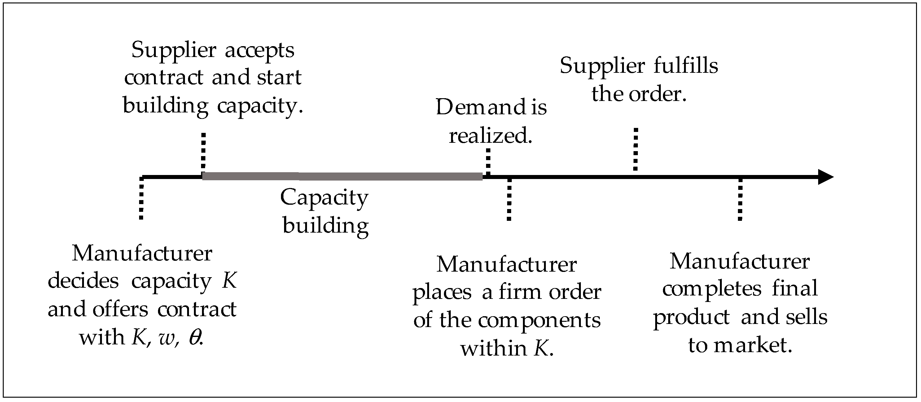
We now explain how we can build a contract to secure an appropriate level of capacity. The sequence of events in the basic model is as follows (see Figure 1 for a graphical illustration).

(1)

The manufacturer determines the production capacity K leading to the maximum system-wide profit. The capacity decision is based on demand forecasts with the parameters related to revenues and costs. Then, the manufacturer offers the supplier a supply contract that includes the production capacity, supply wholesale price w, and the capacity cost-sharing ratio θ (θ = 0 in the basic model) that he is willing to share with the supplier.

(2)

The supplier reviews the contract and decides whether or not to accept it.

(3)

The manufacturer and the supplier start building production capacity K. The production capacity investment cost is proportional to the scale of the production capacity.

(4)

When the sale season arrives, the manufacturer establishes a production plan based on the actual demand and accordingly orders the components from the supplier.

(5)

The supplier produces components in response to the orders from the manufacturer within the production capacity and supplies the components to the manufacturer for wholesale price w.

(6)

The manufacturer completes the finished product with the supplied components and sells it to the market for a sale price p, which is exogenously given in the market.

To have a meaningful supply chain, it is assumed that w > c_s + c_a, p > w + c_m + c_b > c_s + c_m + c_a + c_b. The supplier’s production volume is determined by the production capacity K and the realized demand x. If x ≥ K, the quantity K will be produced and supplied. On the other hand, if x < K, the quantity x will be produced and supplied. Therefore, the production volume of components can be expressed as $\min \left(x,K\right)$, while the excess capacity will be ${\left(K-x\right)}^{+},$ where (y)⁺ = max(y,0). The expectation of the excess capacity, I(K), is obtained as follows:

$$I\left(K\right)=E\left[{\left(K-x\right)}^{+}\right]={{\displaystyle \int }}_0^{K}Kf\left(x\right)dx-{{\displaystyle \int }}_0^{K}xf\left(x\right)dx={{\displaystyle \int }}_0^{K}F\left(x\right)dx$$

(1)

Since the production volume is $\min \left(x,K\right)=K-{\left(K-x\right)}^{+}$, the expected production amount S(K) is as follows:

$$S\left(K\right)=K-{{\displaystyle \int }}_0^{K}F\left(x\right)dx=K-I\left(K\right)$$

(2)

As mentioned previously, the profits of the entire supply chain can be maximized by making decisions on production capacity in the vertical integration environment in which supplied components and finished products are produced by the same company [2]. The profit $P_{sc}$ of the vertically integrated supply chain can be obtained as follows:

$$P_{sc}=\left(p-c_s-c_m\right)\min \left(x,K\right)-\left(c_a+c_b\right)K$$

(3)

Then, the expected profit is as follows:

$$E{P}_{sc}=\left(p-c_s-c_m\right)S\left(K\right)-\left(c_a+c_b\right)K$$

(4)

Taking the first-order derivative of (4) with respect to K gives:

$$\frac{dE{P}_{sc}}{dK}=\left(p-c_s-c_m\right) \overline{F}\left(K\right)-\left(c_a+c_b\right)$$

(5)

where $\overline{F}\left(K\right)=1-F\left(K\right)$. From (5), it is evident that $\frac{dE{P}_{sc}}{dK}$ decreases in K. Hence, $E{P}_{sc}$ is unimodal, and there exists a unique capacity $K_{sc}^{*}$ where the SC profit is maximized, which can be found by solving $\frac{dE{P}_{sc}}{dK}=0$. From (5), $\overline{F}\left(K_{sc}^{*}\right)=\frac{c_a+c_b}{\left(p-c_s-c_m\right)}$. Then, the optimal capacity giving the maximum SC profit is as follows:

$$K_{sc}^{*}=F^{-1}(1-\frac{c_a+c_b}{p-c_s-c_m})$$

(6)

From the system’s perspective, it is optimal to build capacity $K_{sc}^{*}$ to maximize the whole SC profit. The production volume of the final products at the manufacturer is affected by not only its own production capacity, but also the production capacity of the supplier. That is, the manufacturer can fully utilize its production capacity only when the supplier’s capacity is at least $K_{sc}^{*}$. If the supplier’s capacity is smaller than that of the manufacturer, the possible excess capacity of the manufacturer will be lost. On the other hand, if the supplier’s capacity is larger than $K_{sc}^{*},$ the maximum order from the manufacturer will be $K_{sc}^{*}$, which results in the excess capacity of the supplier. Hence, it is reasonable to set the production capacity of the supplier to $K_{sc}^{*}$ identically to that of the manufacturer. Now, we present the CCS contract with appropriate parameters so that the coordinated capacity of the supplier becomes $K_{sc}^{*}$.

4. Capacity Cost-Sharing Contract with Bargaining Power and a Risk-Averse Supplier

This section explains how to establish an optimal coordinated contract using a capacity cost-sharing contract (CCS contract) and introduces a modified CCS contract for risk-averse suppliers in an environment where relative bargaining power is given.

4.1. Capacity Cost-Sharing Contract

The CCS contract contains two parameters, w and θ, which refer to the wholesale price from the supplier to the manufacturer and the fraction of the supplier’s capacity cost that the manufacturer shares with the supplier, respectively. The investment cost at the supplier is shared with the manufacturer; i.e., of the per-unit capacity cost c_a, the manufacturer is responsible for θ c_a, and the supplier for (1 − θ)c_a. In the CCS contract, the profit of the supplier, $P_s$, and the profit of the manufacturer, $P_m$, are as follows:

$$P_s=\left(w-c_s\right)\min \left(x,K\right)-\left(1-\theta \right)c_{a}K$$

(7)

$$P_m=\left(p-w-c_m\right)\min \left(x,K\right)-\left(\theta c_a+c_b\right)K$$

(8)

Then, the expected profits of the supplier and manufacturer are as follows:

$$E{P}_s=\left(w-c_s\right)S\left(K\right)-\left(1-\theta \right)c_{a}K$$

(9)

$$E{P}_m=\left(p-w-c_m\right)S\left(K\right)-\left(\theta c_a+c_b\right)K$$

(10)

The supplier will try to have a supply contract that maximizes its expected profit. The first-order derivative of $E{P}_s$ with respect to capacity K yields:

$$\frac{dE{P}_s}{dK}=\left(w-c_s\right)\overline{F}\left(K\right)-\left(1-\theta \right)c_a$$

(11)

It is straightforward to see that $\frac{dE{P}_s}{dK}$ decreases in K, so there exists a unique capacity $K_{ccs.s}^{*}$ that maximizes the expected profit of the supplier. Then, $K_{ccs.s}^{*}$ can be found by solving $\frac{dE{P}_s}{dK}=0$, which leads to the following expression:

$$K_{ccs.s}^{*}=F^{-1}(1-\frac{\left(1-\theta \right)c_a}{w-c_s})$$

(12)

Now, $K_{ccs}^{*}=K_{sc}^{*}$ should be satisfied to have a coordinated CCS contract. From (6) and (12), the following expression should be satisfied to be globally optimal.

$$\frac{c_a+c_b}{\left(p-c_s-c_m\right)}=\frac{\left(1-\theta \right)c_a}{w-c_s}$$

(13)

If we rearrange (13) with respect to w, we will have the following expression:

$$w=c_s+\frac{\left(1-\theta \right)c_a\left(p-c_s-c_m\right)}{c_a+c_b}$$

(14)

Note that w and θ are negatively proportional to each other in the coordinated CCS contract. In other words, as the wholesale price w increases, the capacity cost-sharing ratio θ should be decreased in the coordinated CCS contract, and vice versa. If components are supplied under a wholesale contract without capacity cost sharing (i.e., θ = 0), expression (14) leads to the optimal wholesale price as follows:

$$w=c_s+\frac{c_a\left(p-c_s-c_m\right)}{c_a+c_b}$$

(15)

Similarly, if the manufacturer is responsible for all of the capacity investment (i.e., θ = 1), the optimal wholesale price will be

$$w=c_s$$

(16)

It is realistic to assume for the CCS contract that the capacity cost-sharing ratio lies between zero and one, i.e., $0<\theta <1$. From (14), this assumption leads to the following relationship in terms of w:

$$c_s\le w\le c_s+\frac{c_a\left(p-c_s-c_m\right)}{c_a+c_b}$$

(17)

From the manufacturer’s perspective, he will try to set the contract parameters to maximize his expected profit. With the same procedure, the optimal production capacity $K_{ccs.m}^{*}$ that maximizes the manufacturer’s profit under the CCS contract is as follows:

$$K_{ccs.m}^{*}=F^{-1}(1-\frac{\theta c_a+c_b}{p-w-c_m})$$

(18)

As in the case of the supplier, for a CCS contract leading to overall SC optimization, the manufacturer’s optimal production capacity $K_{ccs.m}^{*}$ must satisfy $K_{ccs.m}^{*}=K_{sc}^{*}$. From (6) and (18), the following expression should be satisfied to be globally optimal.

$$\frac{c_a+c_b}{p-c_s-c_m}=\frac{\theta c_a+c_b}{p-w-c_m}$$

(19)

If we rearrange (19) with respect to w, we can have the same expression as (14). Hence, we can conclude that assuming that the information needed to determine the capacity is equally known to all the SC stakeholders, a specific set of w and θ involve the coordinated contract parameters for both SC stakeholders.

4.2. Capacity Cost-Sharing Contract with a Bargaining Power

This subsection presents the optimal parameters in the CCS contract when relative bargaining power is given in a two-stage supply chain. Bargaining power refers to the relative ability of SC members to exert influence over each other. We follow the bargaining solution introduced by Iyer and Villas-Boas [9], which takes the manufacturer’s profit-sharing ratio α as the bargaining power, i.e., α = EP_m/EP_sc. From expressions (4) and (10), we can have the following relationship:

$$\mathsf{\alpha }=\frac{E{P}_m}{E{P}_{sc}}=\frac{\left(p-w-c_m\right)S\left(K\right)-\left(\theta c_a+c_b\right)K}{\left(p-c_s-c_m\right)S\left(K\right)-\left(c_a+c_b\right)K}$$

(20)

In the coordinated CCS contract, the capacity cost-sharing ratio θ can be substituted with the wholesale price w by using (13). Then, we have the following expression:

$$\mathsf{\alpha }=\frac{p-w-c_m}{p-c_s-c_m}$$

(21)

Now, given a specific profit-sharing ratio α, the optimal wholesale price is as follows:

$$w=\left(p-c_m\right)-\alpha \left(p-c_s-c_m\right)$$

(22)

Once the optimal wholesale price w is known, the optimal capacity cost-sharing ratio θ can be obtained from (13). Therefore, only one optimal (w, θ) combination satisfies a given profit-sharing ratio. From (22), it is seen that the optimal w decreases with a higher profit-sharing ratio. (This means that the optimal θ increases with a higher α.) From (17) and (21), we can have the following expression in the coordinated CCS contract:

$$1-\frac{c_a}{c_a+c_b}\le \mathsf{\alpha }\le 1.$$

(23)

Expression (23) indicates that when the capacity investment is needed for both the supplier and the manufacturer, channel-coordinated CCS contracts may exist only for a specific range of the profit-sharing ratio α.

4.3. A New CCS Contract for Risk-Averse Suppliers

Thus far, the purpose of decision making is to maximize expected profits assuming that the supplier is risk-neutral. If all SC members are risk-neutral, the combination of (w, θ) obtained in the preceding subsection is channel-coordinated. This subsection presents a modified CCS contract for a supply chain with a risk-averse supplier and a risk-neutral manufacturer when a profit-sharing ratio is given. The risk-averse suppliers consider the profit variability along with the expected profit when making investment decisions. The standard deviation of the profit is used to represent the profit variability. Our contract tries to find the contract parameters to satisfy the following optimization model:

$$\max \mathrm{z}=E{P}_s$$

$$\mathrm{s}.\mathrm{t}. S{P}_s\le \gamma$$

(24)

where SP_s represents the standard deviations of the supplier’s profit and $\gamma$ is a threshold of the profit standard deviation allowed by the risk-averse supplier. Before we introduce the modified CCS contract, the standard deviation of the supplier’s profit should be addressed. The supplier’s production volume is governed by the production capacity K and the random demand x. The variance $\xi \left(K\right)$ of the excess capacity, I(K), is obtained as follows:

$$\xi \left(K\right)=E\left[{\left(K-x\right)}^{+}-E{\left(K-x\right)}^{+}{]}^2=E\right[{\left(K-x\right)}^{+}-I\left(K\right){]}^2$$

(25)

From $E{\left[{\left(K-x\right)}^{+}\right]}^2$ = ${{\displaystyle \int }}_0^K{\left(K-x\right)}^{2}f\left(x\right)dx$= $2{{\displaystyle \int }}_0^K\left(K-x\right)F\left(x\right)dx$, ξ(K) can be expressed as follows:

$$\mathsf{\xi }\left(K\right)=2{{\displaystyle \int }}_0^K\left(K-x\right)F\left(x\right)dx-{[{{\displaystyle \int }}_0^{K}F\left(x\right)dx]}^2$$

(26)

Since the production volume is $\min \left(x,K\right)=K-{\left(K-x\right)}^{+}$, the variance of the production volume is the same as in (26). Then, from (7), (8), and (3), the standard deviation of the profits of the supplier, manufacturer, and supply chain are as follows, respectively:

$$S{P}_s=\left(w-c_s\right)\sqrt{\mathsf{\xi }\left(K\right)}$$

(27)

$$S{P}_m=\left(p-w-c_m\right)\sqrt{\mathsf{\xi }\left(K\right)}$$

(28)

$$S{P}_{sc}=\left(p-c_s-c_m\right)\sqrt{\mathsf{\xi }\left(K\right)}$$

(29)

From (27)–(29), we have the following relationship, which is parallel to the result of Choi et al. [35]:

$$S{P}_{sc}=S{P}_s+S{P}_s$$

(30)

It is seen from (27) that lower w leads to lower SP_s. From the previous discussion, we know that w and θ are negatively proportional in the optimal solution. Hence, to decrease the standard deviation of the supplier’s profit, we need to set a smaller w and larger θ. Now, we introduce the modified CCS contract aiming to secure the maximum profit while satisfying a predefined profit variability level when the profit-sharing ratio α is given.

Modified CCS Contract Algorithm for Risk-Averse Suppliers

Step 0. Input data: p, w, c_s, c_m, c_a, c_b, α, γ, and demand distribution.

Step 1. Obtain the production capacity K from (6) that maximizes the profit of the overall supply chain.

Step 2. Derive a set (w, θ) of the optimal wholesale price and cost-sharing ratio based on the profit-sharing ratio α with which the supplier has the incentive to construct the optimal capacity obtained in Step (1).

Step 3. Calculate the standard deviation of the supplier’s profit $S{P}_s$ for the derived (w, θ) set.

Step 4. If $S{P}_s\le \gamma$ is satisfied, the derived (w, θ) combination is the optimal contract, and the algorithm stops. Otherwise, go to step 5.

Step 5. Find the (w, θ) combination so that $S{P}_s=\gamma$ is satisfied. To that end, first calculate the wholesale price w by using the following expression:

$$w=\frac{\gamma }{\sqrt{\mathsf{\xi }\left(K\right)}}+c_s$$

(31)

With the wholesale price w, the capacity cost-sharing rate θ is obtained from (13). As previously discussed, the standard deviation of the supplier’s profit is proportional to the supply price w, and w and θ are inversely proportional in the optimal (w, θ) combinations. Therefore, in the newly obtained (w, θ) combination, w decreases and θ increases compared to the (w, θ) combination obtained in step 2.

Step 6. The manufacturer pays a fixed transfer amount $T_r$ to the supplier at the time of contracting to satisfy the target profit-sharing ratio. The transfer payment amount is equal to the difference between the supplier’s target profit and the supplier’s expected profit in step 5.

$$T_r=\left(1-\alpha \right)E{P}_{sc}-E{P}_s$$

(32)

In the proposed contract algorithm, the (w, θ) combination and the fixed transfer amount $T_r$ are obtained to maximize the expected profit while limiting the supplier’s profit variability (standard deviation) to a certain level $\gamma$.

5. Numerical Illustration

This section provides an illustrative case to see how the proposed model works in a two-stage supply chain. The base-case scenario is adopted from Mathur [41], in which the demand for the product under consideration during the sales season is assumed to follow a uniform distribution Unif(0, 100), and the contract parameters are p = 10.0, w = 8.0, c_s = 2.0, c_m = 0, c_a = 2.0, and c_b = 0.

First, let us consider a centralized system to determine the globally optimal capacity to maximize the overall profit of the supply chain. The optimal capacity $K_{sc}^{*}$ can be obtained from (6) as follows:

$$K_{sc}^{*}=F^{-1}\left(1-\frac{c_a+c_b}{p-c_s-c_m}\right)=F^{-1}\left(0.75\right)=75$$

By using a special characteristic of the uniform distribution, we can have $I\left(K_{sc}^{*}\right)={{\displaystyle \int }}_0^{K_{sc}^{*}}F\left(x\right)dx=\frac{{\left(75-0\right)}^2}{2\left(100-0\right)}=28.1$ and $S\left(K_{sc}^{*}\right)=K_{sc}^{*}-I\left(K_{sc}^{*}\right)=46.9$ from (1) and (2). The maximum expected profit of the entire two-stage supply chain is obtained from (4) as follows:

$$E{P}_{sc}=\left(p-c_s-c_m\right)S\left(K\right)-\left(c_a+c_b\right)K=8\times 46.9-2\times 75=225.0$$

For the centralized decision, there must be an unbiased decision maker who has the authority to control both stakeholders. However, this is often not the case in industries. Now, suppose that the supply chain under consideration adopts a wholesale contract in a decentralized supply chain environment. The wholesale (WS) contract is a special case of the CCS contract where no capacity cost is shared (i.e., θ = 0). The supplier decides on the optimal capacity to maximize her profit by using (12) as follows:

$$K_{ws.s}^{*}=F^{-1}\left(1-\frac{c_a}{w-c_s}\right)=F^{-1}\left(0.667\right)=66.7$$

With the optimal capacity under the wholesale contract with w = 8.0, the expected profits of the supplier and manufacturer are 133.3 and 88.9, respectively, resulting in 222.2 for the whole supply chain, which is less than the maximum expected SC profit, 225.0, under the centralized decision described above. Figure 2 shows the supplier’s optimal capacity and the profits of the SC stakeholders over varying wholesale prices in the decentralized setting. It is seen in Figure 2a that as the wholesale price increases, the optimal capacity increases. It is also seen that any wholesale price less than the sale price, 10, under the wholesale contract leads to a capacity less than the global optimal capacity, 75. The under-capacity investment under the wholesale contract results in less expected SC profit than 225.0, the maximum expected profit under the centralized decision, as seen in Figure 2b. In the current scenario under the wholesale contract, when the manufacturer sets the wholesale price equal to the sale price, the maximum SC profit is realized. (This is only true when there is no capacity investment cost in the manufacturer. We discuss the implication of the manufacturer’s capacity cost in the latter part of this section.) However, the manufacturer’s profit will be zero with a wholesale price equal to the sale price, so the manufacturer would not offer a contract with zero profit. As a result, a coordinated supply chain decision is impossible due to the double marginalization problems with the wholesale contract in the decentralized system.

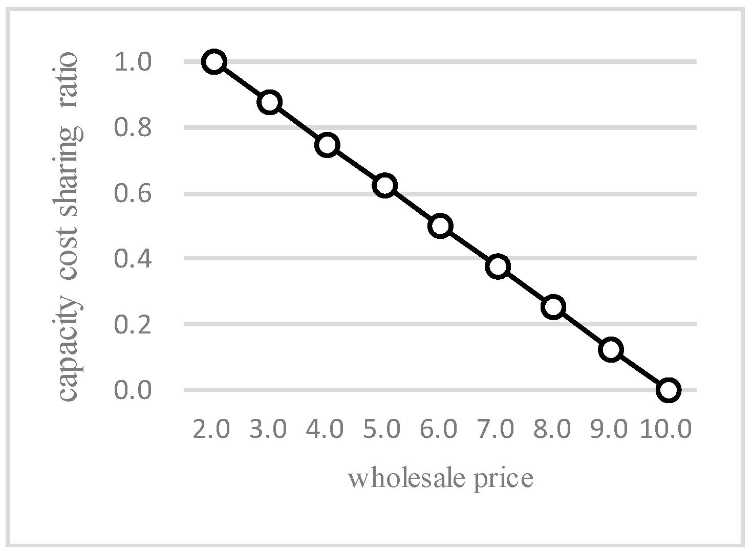
Now, let us consider that the CCS contract is adopted in a decentralized environment. In the present base-case scenario, expression (17) indicates the range of wholesale price w in the optimal (w, θ) combination, i.e., 2.0 < w < 10.0. There are a number of (w, θ) combinations for maximizing the overall supply chain profit in this range of wholesale prices. Figure 3 shows the (w, θ) combinations under which the total SC profit can be maximized. It is seen that θ decreases as w increases in the optimal CCS contract. With a specific w value, only one θ leads to a coordinated solution. For example, in the base-case scenario with w = 8.0, the optimal θ is 0.25 from (13).

Table 2. Optimal (w, θ) combinations for the CCS contract and expected profit for each combination.

Wholesale price w		2.0	3.0	4.0	5.0	6.0	7.0	8.0	9.0	10.0
Capacity cost-sharing ratio θ		1.000	0.875	0.750	0.625	0.500	0.375	0.250	0.125	0.000
Expected profit	Supplier EPs	0.0	28.1	56.3	84.4	112.5	140.6	168.8	196.9	225.0
	Manufacturer EPm	225.0	196.9	168.7	140.6	112.5	84.4	56.2	28.1	0.0
	Supply chain EPsc	225.0	225.0	225.0	225.0	225.0	225.0	225.0	225.0	225.0
	Profit-sharing ratio α	1.000	0.875	0.750	0.625	0.500	0.375	0.250	0.125	0.000

shows some of the optimal (w, θ) combinations, the expected profit of the supplier and the manufacturer for each (w, θ) combination, and the manufacturer’s profit-sharing ratio when the CCS contract is applied. Different (w, θ) combinations lead to different profits for each SC member. It is seen that the profit-sharing ratio α increases as the wholesale price decreases (and equally as the cost-sharing ratio decreases). If a target profit-sharing ratio is given based on a relative bargaining power, an optimal (w, θ) combination can be found, with which the manufacturer designs a coordinated CCS contract. For example, if the target profit-sharing ratio α is 0.75, the optimal (w, θ) combination to maximize the whole SC profit is (4.0, 0.75), as seen in Table 2. If the manufacturer has higher bargaining power, the supply contract is designed with a lower wholesale price and a higher cost-sharing ratio. On the contrary, if the supplier has higher bargaining power, the supply contract is designed with an increased supply price and a reduced cost-sharing ratio.

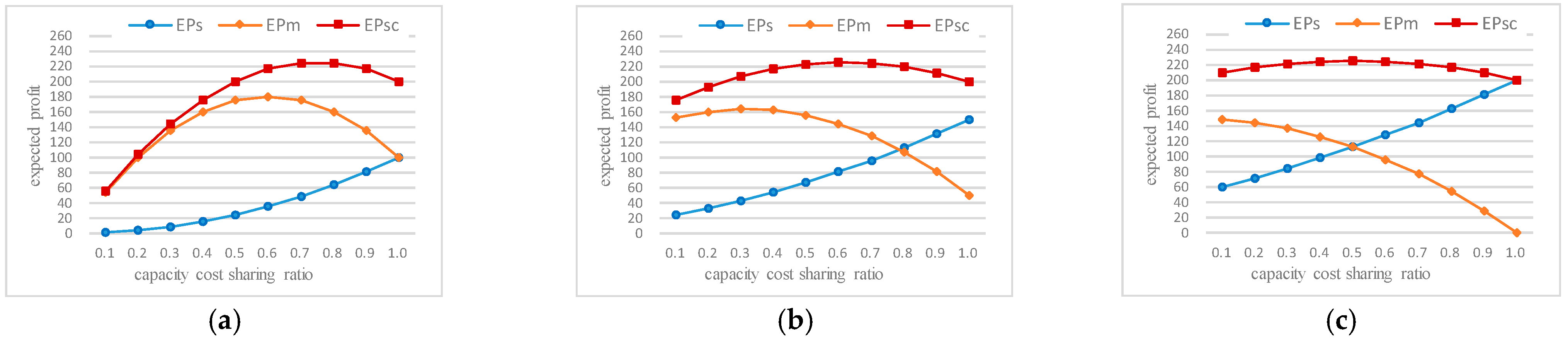
To examine how the cost-sharing ratio θ and wholesale price w affect the profit structure of the supply chain, we conducted experiments using different θ values with different wholesale prices (w = 4.0, 5.0, 6.0). Note that the CCS contracts with (w, θ) combinations (4.0, 0.75), (5.0, 0.625), and (6.0, 0.5) lead to the maximum total SC profit, 225.0. Figure 4 shows that as (w, θ) values deviate from the optimal combinations, the expected profit for the entire supply chain is realized less. The decreased SC profit comes because the supplier’s capacities from the CCS contract with the non-optimal (w, θ) combinations are different from the globally optimal capacity, 75.0. For example, when a CCS contract is designed with (w, θ) = (5.0, 0.4), the capacity for the supplier to build for her maximum profit is 60.0 from (12) (instead of the globally optimal capacity, 75.0). This leads to the SC profit of 216.0 (instead of the maximum profit, 225.0).

As discussed above, when a profit-sharing ratio is given, the combination of the optimal wholesale price and cost-sharing ratio (w, θ) for the entire supply chain is uniquely determined. If the supplier is risk-neutral for the financial risk, the contract can be made by selecting an appropriate (w, θ) combination. However, if the supplier is risk-averse, the volatility (standard deviation) of profits becomes a key decision criterion, along with the expected profits. Now, consider a risk-averse supplier who wants to limit the standard deviation of her profits within 50.0 in an environment where the manufacturer’s profit-sharing ratio is 50%. The followings are the results when the new CCS contract algorithm is implemented.

Step 0. Input data: p = 10.0, c_s = 2.0, c_m = 0, c_a = 2.0, c_b = 0, α = 0.5, γ = 50.0, X~Unif(0, 100).

Step 1. From (6), $K_{sc}^{*}=F^{-1}\left(1-\frac{c_a+c_b}{p-c_s+c_m}\right)=F^{-1}\left(0.75\right)$= 75.

Step 2. From (22), $w=\left(p-c_m\right)-\alpha \left(p-c_s-c_m\right)=10.0-0.5\left(10.0-2.0\right)=6.0$.

From (13), $\theta =1-\frac{(w-c_s)\left(c_a+c_b\right)}{c_a\left(p-c_s-c_m\right)}=1-\frac{4\left(2\right)}{2\left(8\right)}=0.5$. So, (w, θ) = (6.0, 0.5).

Step 3. From (26), $\mathsf{\xi }\left(K\right)=2{{\displaystyle \int }}_0^K\left(K-x\right)F\left(x\right)dx-{[{{\displaystyle \int }}_0^{K}F\left(x\right)dx]}^2$ = 615.2, where ${{\displaystyle \int }}_0^{K}F\left(x\right)dx=\frac{{\left(K-0\right)}^2}{2\left(100-0\right)}=28.1$, ${{\displaystyle \int }}_0^{K}xF\left(x\right)dx=\frac{1}{\left(100-0\right)}\left(\frac{1}{3}{K}^3\right)=1406.0$.

From (27), $S{P}_s=\left(w-c_s\right)\sqrt{\mathsf{\xi }\left(K\right)}=4\sqrt{615.2}$ = 99.2.

Step 4. The condition $S{P}_s\le \gamma =50$ is not satisfied. So, go to step 5. (If this condition were satisfied, the current (w, θ) = (6.0, 0.5) combination would be optimal.)

Step 5. From (31), $w=\frac{\gamma }{\sqrt{\mathsf{\xi }\left(K\right)}}+c_s=\frac{50}{\sqrt{615.2}}+2.0=4.02$.

From (13), $\theta =1-\frac{\left(w-c_s\right)\left(c_a+c_b\right)}{c_a\left(p-c_s-c_m\right)}=0.748$. Hence, the new (w, θ) = (4.02, 0.748).

Step 6. From (32), transfer amount $T_r=\left(1-\alpha \right)E{P}_{sc}-E{P}_s=\left(1-0.5\right)225-56.7=55.8$.

When the CCS contract is concluded, the manufacturer pays the fixed amount of 55.8 to the supplier. Consequently, the two SC members share the total SC profit by 50% each (α = 0.5), while the standard deviation of the supplier’s profit is confined within a specific limit, 50.0.

So far, our investigations have been done with c_m = 0 and c_a = 0, which means that no production and capacity costs are incurred by the manufacturer. These cost factors can be included in our model. Now, let us consider our original scenario with these cost factors with c_m = 0.2 and c_a = 0.3. Then, the $K_{sc}^{*}$ can be obtained from (6), $K_{sc}^{*}=F^{-1}\left(0.705\right)=70.5$, and the SC’s maximum expected profit is 19.0, obtained from (4). When the wholesale contract is applied, the optimal wholesale price is 8.78, obtained from (9), resulting in an expected SC profit of 193.9, expected supplier profit of 168.6, and expected manufacturer profit of 25.3. Note that the wholesale contract can provide an optimal solution for maximizing the SC’s expected profit when the manufacturer’s capacity cost is involved. However, the profit-sharing ratio is fixed in the optimal wholesale contract, which is not acceptable by some SC members. In our CCS-based contract model, we can set the contract parameters for the optimal solution given a bargaining power with a profit-sharing ratio. For example, given the profit-sharing ratio α = 0.5, the optimal wholesale price and capacity cost-sharing ratio are w = 5.9 and θ = 0.425, respectively. In this contract, the SC’s expected profit of 193.9 is divided between the two SC members, 97.95 each. In the current scenario, the optimal solution is found for a specific range of profit-sharing ratios, i.e., 0.13 ≤ α ≤ 1.0, from (23). If α < 0.13, optimal capacity cost-sharing ratio θ is negative. For example, with α = 0.1, the maximum SC profit is realized with θ = −0.035, which means that the supplier secures the capacity at her own expense and pays a certain amount to the manufacturer. This is a contract that is unlikely to happen in real-world industries.

6. Conclusions

This study deals with a two-stage supply chain where the manufacturer buys components from the supplier, uses them to make final products, and sells them. To develop and launch a new product, both the manufacturer and the supplier must secure production capacity in advance. Bargaining power is recognized by practitioners as an important consideration governing the relationship between supply chain members [9]. This paper addresses the supply contract problems governed by bargaining power, which has been ignored in the existing literature. We present a capacity cost-sharing (CCS) contract for a supply chain in which the bargaining power is considered. We show how to determine the contract parameters, including the wholesale price w and capacity cost-sharing ratio θ, under a given bargaining power for the coordinated contract. The effect of the different (w, θ) combinations on the profits of the supplier and manufacturer is investigated. We show that the wholesale price w and capacity cost-sharing ratio θ are negatively proportional to each other, and the manufacture’s expected profit increases as θ (w) increases (decreases) in the coordinated CCS contract. Another key finding is that there exists a CCS contract leading to a coordinated supply chain for a specific range of bargaining power when the capacity investment is needed for both the supplier and the manufacturer. This paper also considers a supply chain with a risk-averse supplier. A new CCS contract is presented where the volatility of the supplier’s profit is included in the design of the contract. Numerical illustrations are provided to clarify how the contract parameters are determined in the proposed CCS contract and to examine the effect of the contract parameters on SC performance.

Our study has some limitations and could be extended in several directions. First, in the current study, it is assumed that all of the information is shared among the SC members. In industries, some information is confidential to other SC members, and so some of the information is not shared among the SC members. The coordination of the supply chain with asymmetric information is an interesting problem to be addressed. Second, in this study, all of the parameters are deterministic, except for the demand. In reality, some other parameters are not deterministic. For example, the market price may be not known in advance, but may rather be variable depending on the market situation in the sale season. A study on stochastic features may be required. Third, the development of an effective supply contract model considering newly updated demand information will become a practical research theme in a situation where the accuracy of demand forecasting increases as the sale season approaches. Fourth, even though this paper mainly considers the risk caused by the volatility of demand, a topic that includes supply risks is an interesting area to be studied. Fifth, the current study may expand to a supply chain with multiple suppliers with different risk preferences. In this case, multiple types of contracts may be designed by the manufacturer where the risk-pooling concept is a key issue. Finally, this paper uses a simple SC scenario for numerical analysis. We hope that our study provides a supply contract framework that can be empirically tested using real-world industrial data.