Impacts of Real-Time Traffic State on Urban Expressway Crashes by Collision and Vehicle Type

Abstract

With the rapid development of urban expressway systems in China in recent years, traffic safety problems have attracted more attention. Variation of traffic flow is considered to have significant impact on the safety performance of expressways. Therefore, the motivation of this study is to explore the mechanism of how the variation of traffic flow measurements such as average speed, speed variation and traffic volume impact the crash risk. Firstly, the crashes were classified according to crash type and vehicles involved: and they are labeled with rear-end collisions or side-impact collisions, they are labeled with heavy-vehicle related collisions or light-vehicle related collisions as well. Then, the corresponding crash data were aggregated based on the similarity of traffic flow conditions and types of crashes. Finally, a random effect negative binomial model was introduced to consider the heterogeneity of the crash risk due to the variance within the traffic flow and crash types. The results show that the significant influencing factors of each type of crashes are not consistent. Specifically, the percentage of heavy vehicles within traffic flow is found to have a negative impact on rear-end collisions and light-vehicle-related collisions, but it has no obvious correlation with side-impact collisions and heavy-vehicle-related collisions. Average speed, speed variation and traffic volume have an interactive effect on the crash rate. In conclusion, if the traffic flow is with higher speed variation within lanes and is with lower average speed, the risk of all types of crashes tends to be higher. If the speed variation within lanes decreases and the average speed increases, the crash risk will also increase. In addition, if the traffic flow is under the conditions of higher speed variation between lanes and lower traffic volume, the risk of rear-end collisions, side-impact collisions and heavy-vehicles related collisions tend to be higher. Meanwhile, if the speed variation between lanes decreases and the traffic volume increases, the crash risk is found to increase as well.

1. Introduction

With the fast rapid development and improvement of traffic detection and information communication technology, collecting massive amounts of and high-precision real-time traffic flow and crash data is becoming much easier. Therefore, the research on the relationship between crashes and real-time traffic flow data has attracted extensive attention [1,2,3] in recent years. Identifying traffic conditions with a high crash risk can provide strong support for the formulation of crash early warning strategies during practical traffic operations.

The influence of traffic flow characteristics on crash frequency has been extensively studied, which provides useful insights for formulating effective traffic safety improvement measures. Previous studies suggest that there is a certain correlation between speed and speed variance and the occurrence of crashes [4,5,6], but their results show that the impact of speed-related measurements on crash rates is different between each other. Studies show a positive relationship between speed and speed variation with crash rates [4,7], as the research results of Wang’s study [4] show that if the average speed of urban arterials increased by 1%, the crash frequency will increase by 0.7%, and the crash frequency will increase with the increase of speed variation. Choudhary divided crashes into heavy/light-vehicle crashes and killed or serious/slight-injury crashes, and the results show that the crash rates of these four types of crashes increase with the increase of speed and speed variance [7]. Abdel-Aty studied the influencing factors of rear-end collisions, and the results showed that the average speed is positively correlated with crash frequency under high-speed conditions [8]. On the other hand, under low-speed conditions, the crash risk will be high if there is a large variation in speed. Imprialou finds that single-vehicle crashes and multiple-vehicle casualties are related to high speed and low traffic flow, while the property-damage-only crashes involving multiple vehicles are not correlated with high speed but are related to traffic congestion [9]. However, there is also a view that the average speed are not correlated with the crash risk, but higher speed variation will lead to more crashes [10]. Moreover, studies have found that the average vehicle speed is negatively correlated with the risk of crashes [11].

The conflicting conclusions above may be the result of different modeling methods, data sources and/or low data quality. In addition, the road environment is found to be an important moderator of the impact of speed-related variables on crash rates [12]. Cameron suggests that the Nilsson’s model should not be applied to urban arterial roads directly. In urban arterials, the mean speed needs to be supplemented by the speed variation because the former is weak in representing the influence on casualty crashes. Using urban expressways of Shanghai, China for a case study, Yu revealed crash occurrence mechanisms, such as variations of volume and speed drops, that increase crash occurrence likelihood during weekday peak hours [13]. Chen suggests that the crash likelihood increases when the traffic speed is significantly different from the legal speed limit on the I-25 corridor in Colorado [14]. A similar conclusion was found by Theofilatos’s finding that traffic variations were found to significantly influence accident likelihood on urban arterials [15]. Therefore, it can be concluded from the above studies indicate that developing refined models based on crash types and road types can help to better understand the mechanisms of crashes [16,17]. However, so far, there are only a few studies that have been conducted to study the relationship between real-time traffic variations and crashes split by collision types (rear-end collision, side-impact collision, etc.) and vehicle types (heavy and light-vehicle crashes), especially in context of urban expressway.

In recent years, scholars have discussed the impact of data aggregation methods on crash frequency modelling. In the previous research, two crash data aggregation methods were mainly used, namely segment-based and condition-based crash data aggregation methods. The segment-based method has been widely used in crash frequency prediction research such as in the “Highway Safety Manual” [18]. This method studies the relationship between crash frequency and average traffic conditions represented by annual average daily traffic (AADT). However, it has certain shortcomings in assessing the impact of traffic variations onto crashes in a short period of time [19,20]. Recently, some scholars [7,9,21,22] have found that when the crash data are aggregated according to the similarity of the traffic condition prior to the occurrence of the crash, the modelling results are more reliable than the traditional segment-based method. Choudhary analyzed the traffic flow conditions within 5 min before each reported crash time collected by the upstream detector closest to the crash location and found that a higher speed variance resulted in more crashes [7]. Yu compared the two methods and found that the condition-based method is more reasonable for crash risk analysis [21]. Choudhary found that the condition-based method can increase the understanding of the crash-related factors and help the assessment and formulation of road safety measures by identifying the traffic flow conditions that are prone to crashes [7].

The counting model in statistics has often been used for crash frequency modelling. The Poisson regression model and negative binomial regression model are the two frequently used methods [23,24]. Among them, the negative binomial model has been widely used for solving the problem of over-dispersed data. Although the modelling and analysis methods are continuously optimized and improved, there are still many unresolved or easily overlooked problems [25,26], such as those related to data heterogeneity and aggregation. Random effect negative binomial model is found to be a better choice over other models because it accounts for over-dispersion and heterogeneity in the data [26,27,28,29,30].

In summary, the above-mentioned studies mainly analyze the direct correlation between traffic speed or volume and crash risk. Previous studies found that traffic speed or volume has a significant positive or negative correlation with crash risk, while conflicting conclusions also exist. To some extent, the interactive impact of traffic variation onto road safety is still unclear, which, in turn, requires further in-depth and systematic analysis. In modeling the impact of traffic state, only a few of previous studies considered crash types or crash vehicles, and they basically ignored the potential effect of data aggregation and data heterogeneity on crash prediction. Therefore, in order to address the heterogeneity issues of traffic variations, a random effect negative binomial model is introduced to study the relationship between traffic variation and crash frequency on urban expressways in this paper. An aggregation method for the crash data based on the similarity of traffic flow conditions is used to study the occurrence mechanism of various crashes. It is believed that the results from this paper should be able to provide theoretical support for real-time early warning of road safety, particularly for urban expressways.

2. Data and Methodology

Previous studies show that many factors could influence crash rate of different types of roads, without exception to urban arterial. Traffic conditions may also be affected by the traffic signal control and other traffic management countermeasures. As a result, the relationship between traffic variations and crash rate on expressways is considered with a strong connection and therefore such a relationship is fully studied in this paper. This paper first analyzes the aggregated crash data and concurrent traffic data. Then, the predictive models are developed using selected variables. After that, the model validation is carried out.

2.1. Collection of Crash and Traffic Data

Detailed crash data and real-time traffic flow data are used to study the impact of traffic variations on crashes. The urban expressway studied is located inside the City of Wuhan and it is a part of the Third Ring Road of the city, with a total length of 37 km, and it is installed with similar guardrail and central median. The alignment radius and road control of the tested corridor are consistent with those required under the design speed of 80 km/h; no obvious changes in road factors are found along the test segment, which mainly carries truck traffic, compared to other urban arterial roads. In addition, the highways selected for our study underwent safety audits during design and construction and potential road risks are removed prior to the opening according to the Design Specifications for Highway Safety Facilities and other standards. As a results, the effects of road geometric design, weather condition and other factors on crash rates are not considered in this study.

Microwave traffic flow detectors are set along the studied segments for collecting real-time traffic flow data. The studied segment is designed with divided, two-way, six lanes or eight lanes, with a design speed of 80 km/h and a corresponding maximum traffic capacity of 2100 pcu/h/lane. The heavy vehicles are restricted to driving in the third (for two-way six lanes segments) or third and fourth lane (for the two-way eight lanes segments). The data collection took place in the following two periods, from 1 September 2018 to 31 November 2018 and from 1 March 2019 to 31 May 2019. The maximum peak hour of traffic flow is 1784 pcu/h/lane with an average off-peak flow of 772 pcu/h/lane. Average traffic volume on and off ramps is 168 pcu/h and 152 pcu/h. The corresponding maximum travel speed is 78 km/h, with an average speed of 52 ± 15 km/h. The selected expressway segment is mostly operating at the Level of Service of B or C. No serious congestion is found during the above periods.

The crash data are extracted from the traffic crash database of the traffic management department of the city, and their detailed information are also recorded, such as the location, time and type of the traffic crash. A total of 1188 crashes occurred during the study, of which rear-end collisions and side-impact collisions accounted for 54% and 41%, respectively. The two types of crashes account for 95% of the total, which constitute the majority of the crashes taking place on the urban expressway studied. Vehicles are divided into heavy vehicles and light vehicles according to the Chinese Automobile Classification Standard. In terms of the types of vehicles involved in crashes, once a heavy vehicle is involved, the crash is counted as a heavy vehicle crash with 353 crashes, whereas the other 835 crashes involve only light vehicles. A large proportion of crashes involve heavy vehicles, which poses significant safety risks to the users of the facility. The real-time traffic flow data is collected by a set of microwave traffic flow detectors installed along the facility. There are 27 sets of detectors along the urban expressway under study, with an average deployment distance of about 1.37 km, which can collect the following real-time traffic data, such as vehicle passing time, speed, vehicle type on each lane. The traffic flow measurements, including average speed, traffic volume, proportion of heavy-vehicles, speed variation among lanes and within each lane with regards to each crash type and collision vehicle type are collected every 5-min and summarized in

Table 1. Summary statistics of traffic flow measurements per 5 min with regards to crash and collision vehicle type.

Crash Type	Variable	Mean	SD	Max	Min
All collisions	Crash Frequency	1188
	Average speed (km/h)	51.74	14.66	77.52	10.15
	Traffic volume (pcu)	64.36	29.08	148.66	5.00
	Heavy-vehicle proportion (%)	4.15	6.16	65.52	0.00
	Speed variation between lanes (km/h)	4.46	3.14	26.38	0.55
	Speed variation within lanes (km/h)	5.50	3.96	39.68	0.27
Rear-end collisions	Crash Frequency	646
	Average speed (km/h)	51.82	13.08	73.40	10.15
	Traffic volume (pcu)	69.69	26.40	148.66	5.00
	Heavy-vehicle proportion (%)	3.30	4.27	56.01	0.00
	Speed variation between lanes (km/h)	4.45	2.88	24.31	0.55
	Speed variation within lanes (km/h)	5.16	3.74	39.50	0.45
Side-impact collisions	Crash Frequency	489
	Average speed (km/h)	54.17	12.41	77.72	11.73
	Traffic volume (pcu)	60.11	27.87	148.33	5.25
	Heavy-vehicle proportion (%)	5.26	8.22	86.36	0.00
	Speed variation between lanes (km/h)	4.51	2.72	26.39	0.61
	Speed variation within lanes (km/h)	6.12	4.15	39.68	0.30
Heavy-vehicle-related collisions	Crash Frequency	353
	Average speed (km/h)	53.20	13.64	77.51	11.85
	Traffic volume (pcu)	56.34	26.41	139.67	5.25
	Heavy-vehicle proportion (%)	6.14	9.42	86.36	0.00
	Speed variation between lanes (km/h)	4.70	2.82	26.39	0.61
	Speed variation within lanes (km/h)	6.18	3.50	23.88	0.30
Light-vehicle-related collisions	Crash Frequency	835
	Average speed (km/h)	52.79	12.60	73.40	10.15
	Traffic volume (pcu)	69.22	27.22	148.67	0.00
	Heavy-vehicle proportion (%)	3.36	4.07	56.25	0.00
	Speed variation between lanes (km/h)	4.40	2.84	24.32	0.55
	Speed variation within lanes (km/h)	5.36	4.11	39.68	0.43

.

2.2. Data Processiong and Filtering

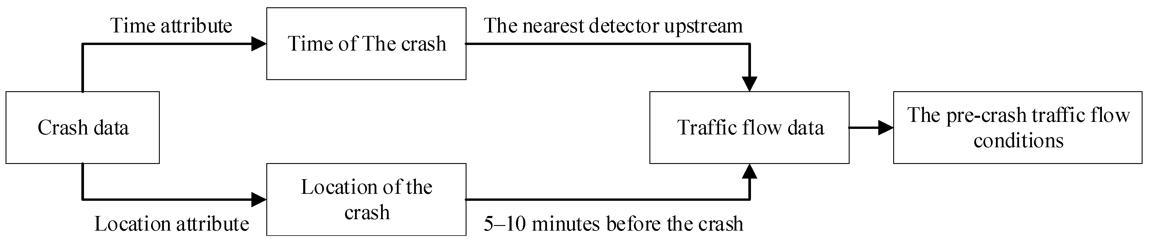
Previous studies show that traffic flow condition prior to the crash is closely related to the occurrence of the crash. For instance, Oh collected real-time traffic flow data through upstream loop detector ahead of the crash occurrence location and used the traffic flow data just 5 min prior to the crash report time to identify the crashes [31,32]. Abdel-Aty concluded that the speed variation that is detected from the closest loop detector within 5–10 min’ interval prior to the crash report time has most significant impact on the crashes [33,34]. Based on these experiences, the pre-crash traffic flow conditions in this study are defined as those 5–10 min prior to the reported crash time, which are collected by the closest detectors upstream to the crash location. To improve the reliability of the modelling results, crashes more than 800 m away from the detectors were screened out, considering that the average distance between the detectors in the previous research is around 800 m [2,7,21] The workflow of data collection is shown in Figure 1. The relevant traffic flow data is determined and extracted by the occurrence time of related crash(s), and in this way, the corresponding detectors for collecting relevant traffic flow data is selected according to the location of the crash, aiming to identify traffic flow conditions before the crash, as shown in Figure 1. For example, if a traffic crash happened at 12:44 on 20 September 2018, then traffic flow data of the nearest microwave traffic flow detector upstream of the crash location, within the interval of 12:34–12:39 p.m., is extracted and used to develop the corresponding crash prediction models.

For the urban expressway studied, raw traffic flow data of each lane was recorded and aggregated at 5-min interval. However, traffic flow data collected often contain abnormal and missing values because of data noise and hardware equipment failure. It is necessary to clean such kind of data to avoid the negative impact of abnormal data on the model. The abnormal data, shown as wrong or missing traffic volume and speed, due to data noise and equipment failure are quite different from the normal data. Therefore they cannot be used to study any rules. Therefore, the threshold and logical reasoning method are combined to detect abnormal data. In this study, all invalid and unrealistic values are excluded from the further analysis, and the rules for excluding outliers include: (1) “missing or outlier” records in the raw data; (2) speed < 0 km/h or speed > 100 km/h; (3) traffic volume < 0 pcu, or traffic volume > 150 pcu in five minutes; (4) number of lanes > 5; (5) Heavy-vehicle proportion < 0.

2.3. Variable Selecting and Setting

This study uses the following five variables, including the average traffic volume per lane, the proportion of heavy vehicles, the average speed, the speed variation between lanes and the speed variation within each lane, to study the relationship between traffic variations and the risk of crashes. It should be noted that in the following data analysis steps, traffic volume of various types of vehicles is converted into the Passenger Car Unit (PCU) according to the defined conversion coefficient. In addition, the original traffic flow data is aggregated into 5-min units to remove the impact of occasional flow fluctuation.

Traffic volume $q$: average traffic volume per lane in five-minute period:

$$q=\frac{1}{L}{{\displaystyle \sum }}_{l=1}^L{q}_l$$

(1)

where $q$ stands for the traffic volume, $L$ is the number of lanes and $q_l$ is the PCU value for a five-minute period on each lane.

Heavy-vehicle proportion $w$: the proportion of heavy vehicles refers to the proportion of heavy vehicles that passes through a segment in a five-minute period.

$$w=\frac{Q^{\prime }}{Q}\times 100\%$$

(2)

where $Q^{\prime }$ is the number of heavy vehicles and $Q$ is the summation of the number of vehicles in a five-minute period.

Average speed $v$: The average speed of all the vehicles that present on a road section along one traveling direction in a five-minute period.

$$v=\frac{1}{Q}{{\displaystyle \sum }}_1^Q{v}_Q$$

(3)

where $v_Q$ is the speed of each vehicle.

The speed variation between lanes $v^{\prime }$: for each one-minute interval, the standard deviation of speeds between the lanes was calculated, and then the average of these standard deviations for 5 min was considered as the between-lanes speed variation.

$$v^{\prime }=\frac{1}{T}{{\displaystyle \sum }}_1^T(\sqrt{\frac{{{\displaystyle \sum }}_1^L(v_{l,t}-\overline{v_t}{)}^2}{L}})$$

(4)

where $\overline{v_t}$ is the average speed for all lanes for minute t and $v_{l,t}$ is the average speed for the $lth$ lane for minute t, and T is the number of the lanes.

The speed variation within lanes $v^{″}$: for each lane, the standard deviation of speeds for a 5 min interval was calculated, and then the average of these standard deviations for all three lanes was considered as within the lane speed variation.

$$v^{″}=\frac{1}{L}{{\displaystyle \sum }}_1^L(\sqrt{\frac{{{\displaystyle \sum }}_1^T(v_{l,t}-\overline{v_l}{)}^2}{T}})$$

(5)

where $\overline{v_t}$ is the average speed for 5 min within lane $l$.

2.4. Data Aggregation

In this paper, the impact of traffic states on crash frequency is investigated under different traffic flow conditions, and each traffic flow condition is defined as a crash scenario. Thus, a total of 432 crash scenarios (i.e., 4 levels of average speed × 4 levels of traffic volume × 3 levels of speed variation between lanes × 3 levels of within-lane speed variation × 3 levels of heavy-vehicle proportion) is developed, covering all possible traffic flow scenarios that may lead to crashes, and each scenario represents a unique traffic condition. The crash frequency in each scenario was represented by a combination of crash type (Rear-end collisions and Side-impact collisions) and vehicle type (Heavy-vehicle related collisions and Light-vehicle related collisions). The crash data grouped into the same scene was aggregated to form an analysis dataset, and the median of each traffic variable in each group is used to represent the corresponding traffic condition. In addition, the average vehicle-hour spent for going through the testing segment of each scenario is introduced as an exposure variable to calculate the probability of crashes under a specific traffic flow condition.

$$VH{T}_i=q_i·t_i=q_i·\frac{1}{v_i}$$

(6)

where, $VH{T}_i$ represents the average vehicle-hour travelled per kilometer in the ith scenario; $q_i$ is the traffic volume under the corresponding scenario; $v_i$ is the average speed under the same scenario.

2.5. Crash Predicition Modelling

Traditional count models for crash frequency prediction include Poisson regression model and Negative Binomial distribution model, and the Negative Binomial distribution models have been widely used to work around the over-dispersion issues inherent in count data. Similar to previous studies, the crash frequency data aggregated based on traffic condition are assumed to follow the negative binomial distribution in this paper:

$$y_{ik} ~ Negative Binomial\left({\lambda }_{ik},\alpha \right)$$

(7)

where ${\lambda }_{ik}$ and $y_{ik}$ refer to the expected crash frequency and the observed crash frequency for collision type $k$ of the scenario $i$, respectively, and $\alpha$ represents the over-dispersion parameter.

To describe the unobserved heterogeneity of the modeling data, a random effect term ${\phi }_{ik}$ was introduced into the negative binomial model, as follows:

$$\ln \left({\lambda }_{ik}\right)={\beta }_{k0}+{\displaystyle \sum }_{m=1}^m{\beta }_{km}{X}_{ikm}+\ln \left(e_i\right)+{\phi }_{ik}$$

(8)

$${\phi }_{ik}~N\left(0,{\sigma }_{\phi }^2\right)$$

(9)

where ${\beta }_{k0}$ represents the intercept of crash type $k$, ${\beta }_{km}$ is the coefficient of mth explanatory variable for crash type $k$,$e_i$ is the value of exposure variable for ith observation, $X_{ikm}$ is the value of mth explanatory variable for ith observation for crash type $k$ and ${\phi }_{ik}$ is the unobserved heterogeneity for ith observation for crash type $k$, which follows the normal distribution with a mean value of zero and a variance of ${\sigma }_{\phi }^2$.

2.6. Prediciton Performance Evaluation

Akaike Information Criterion (AIC) is the main statistic to check the goodness-of-fit of the models developed in this paper. The smaller value of AIC information criterion indicates the better goodness-of-fit. The BIC information criterion is usually used as a supplement to the AIC information criterion. The smaller value of the BIC information criterion indicates a better fit of the model.

To evaluate the accuracy of the predicted results, two indicators were introduced: Mean Absolute Deviation (MAD) and Mean Squared Error (MSE). MAD describes the average deviation between the predicted and the observed crash frequency under each scenario, and the MSE refers to the average deviation squared. The smaller value of MAD and MSE mean a higher prediction accuracy of the model. Besides, $R^2$ is introduced to describe the accuracy of the model, and its value ranges from 0 to 1. A higher value of $R^2$ means a better model fit. Literature indicates that when $R^2$ is greater than 0.4, the developed model is considered to have a good fit.

$$\mathrm{MAD}=\frac{1}{n}{\displaystyle \sum }_{i=1}^n\left|y_{ik}-{\lambda }_{ik}\right|$$

(10)

$$\mathrm{MSE}=\frac{1}{n}{\displaystyle \sum }_{i=1}^n{\left(y_{ik}-{\lambda }_{ik}\right)}^2$$

(11)

$$R^2=\frac{{{\displaystyle \sum }}_{i=1}^n{\left({\lambda }_{ik}-\overline{y_{ik}}\right)}^2}{{{\displaystyle \sum }}_{i=1}^n{\left(y_{ik}-\overline{y_{ik}}\right)}^2}$$

(12)

where $\overline{y_{ik}}$ is the observed average crash frequency for $k$ crash type of the scenario $i$.

3. Results

3.1. Analysis of Traffic Flow and Crash Data

Analysis and visualization of the above variables reveals that the traffic flows show very interesting temporal distribution characteristics, as shown in Figure 2. For instance, traffic volume data collected on the site clearly presents a morning and evening peak, as demonstrated in Figure 2a. The proportion of heavy vehicles is lower in the daytime and much higher at nighttime and early mornings, which is related to the travel restriction policies regarding heavy vehicles of the urban expressways, as shown in Figure 2b. Figure 2c shows the changes in the speed variation among lanes and the within-lane speed variation over time. The two variables are higher at nighttime and early mornings. The lower traffic volume and larger speed variation at those times may be the reason for such an observation.

Pre-crash traffic conditions are extracted and then combined with the historical traffic crash data. For each traffic variable, it is defined as follows. To be specific, the average speed was firstly divided into 4 equal levels with each level covering 25% of its cumulative distribution, then the dataset for each average speed division is divided into 4 equal parts according to the cumulative distribution of traffic volume. Similarly, the speed variation between lanes for each separate traffic volume quantile is divided into 3 again; the speed variation within lanes for each speed variation between lanes division was divided into 3; and the heavy-vehicle proportion for each speed variation within lanes division was divided into 3 as well. After data aggregation, there is 432 traffic scenarios. The summary statistics of the scenario-based dataset are shown in

Table 2. Summary statistics of the scenario-based data set.

Variable	Description	Mean	SD	Min	Max
Average speed (km/h)	Median speed for the crash occurrence scenario	50.31	15.90	4.85	76.00
Traffic volume (pcu)	Median volume per lane in 5 min intervals for the crash occurrence scenario	41.56	25.92	6	101.25
Heavy-vehicle proportion (%)	Median heavy-vehicle proportion in 5 min intervals for the crash occurrence scenario	11.36	11.78	0	55.56
Speed variation between lanes (km/h)	Median between-lanes speed variation in 5 min intervals for the crash occurrence scenario	6.19	4.25	0.39	23.84
Speed variation within lanes (km/h)	Median within lane speed variation in 5 min intervals for the crash occurrence scenario	4.62	2.96	0.66	23.56
Crash frequency per 5 min interval	Rear-end collisions	1.47	1.99	0	15
	Side-impact collisions	1.09	1.23	0	8
	Heavy-vehicle-related collisions	0.77	0.95	0	7
	Light-vehicle-related collisions	1.91	2.42	0	17

.

3.2. Negative Binomial Model

Different combinations among the above independent variables are tested for developing the optimal models, in order to control the possible interactions among independent variables. Based on the criteria of minimum AIC, the best combination of independent variables is selected.

Table 3. Estimation results of random effect negative binomial model.

Variables	Rear-End Collisions		Side-Impact Collisions		Heavy-Vehicle-Related Collisions		Light-Vehicle-Related Collisions
	Mean	p Value	Mean	p Value	Mean	p Value	Mean	p Value
Intercept	−6.4276	0.0000	−5.9460	0.0000	−6.4090	0.000	−5.9740	0.0000
Average speed	0.0801	0.0000	0.0706	0.0000	0.0784	0.0000	0.0804	0.0000
Traffic volume	0.0258	0.0000	0.0139	0.0386	/	/	0.0231	0.0000
Speed variation between lanes	0.1939	0.0000	0.0961	0.0129	0.1939	0.0034	0.1807	0.0000
Speed variation within lanes	0.6270	0.0000	0.4871	0.0000	0.5092	0.0005	0.6260	0.0000
Heavy-vehicle proportion	−6.4851	0.0000	/	/	/	/	−6.8611	0.0000
Average speed * Speed variation within lanes	−0.0124	0.0000	−0.0075	0.0004	−0.0074	0.0047	−0.0105	0.0000
Volume * Speed variation between lanes	−0.0041	0.0000	−0.0021	0.0010	/	/	−0.0039	0.0000
Average speed * Speed variation between lanes	/	/	/	/	−0.0031	0.0100	/	/
ln(exposure)	1
AIC	1353.1		1321.7		1120.9		1549.3
BIC	1393.5		1357.5		1152.2		1589.6
MAD	0.85		1.04		0.58		1.02
MSE	2.73		1.93		0.79		3.28
$R^2$	0.81		0.85		0.76		0.83

Note: * means “the results given are considered the impact of these two factors”.

shows the posterior estimation of the random effect negative binomial model based on the crash scenario dataset. The estimated parameters are statistically significant based on their 95% significance levels.

According to the estimation results for the rear-end collision and side-impact collision prediction models, the significant independent variables finally included inside the models are: average speed (Mean = 0.0801, p value = 0.00 < 0.05), traffic volume (Mean = 0.0258, p value = 0.00 < 0.05), speed variation among lanes (Mean = 0.1939, p value = 0.00 < 0.05), within-lane speed variation (Mean = 0.6270, p value = 0.00 < 0.05), interaction terms between average speed and speed variation within lane (Mean = −0.0124, p value = 0.00 < 0.05), and interaction terms between traffic volume and speed variation between lanes (Mean = −0.0041, p value = 0.00 < 0.05). Different from the side-impact collision model, the heavy-vehicle proportion is also a significant independent variable for the rear-end collision model (p value = 0.00 < 0.05). Its coefficient is negative (Mean = −6.4851), indicating that it has a negative impact onto the crash risk. According to the analysis of traffic variation patterns of heavy vehicles, the number of heavy vehicles traveling at nighttime and early mornings in the studied area is much higher than that during the daytime. However, the majority of recorded crashes occurred during daylight hours, which may explain the inverse relationship between the proportion of heavy vehicles and the crash rate.

$R^2$ When analyzing the relationship between the crash frequency and related independent variables, such as traffic volume and average speed, their effects on crashes cannot be analyzed separately due to their combined interaction effects. As shown in Figure 3, the relationship between the average speed, the speed variation within lane and the crash rate was plotted. In the case of a combination of higher speed variation within lane and a lower average speed (or vice versa), the curve line becomes very steep, indicating that the crash rate increases very quickly under such a scenario. There is a high-speed variation in the same lane combined with a low average speed and it may indicate that the roadway is in a congested traffic flow condition with vehicles taking frequent stop-and-go actions. Due to the limited distance between vehicles, the driver’s response time to a sudden speed change of front vehicle is reduced, so it leads to more rear-end collisions. On the other hand, higher average speed and lower within-lane speed variation increase the crash risk, which is mainly reflected by the impact of higher average speed on the crash risk. When the vehicle is operating at a higher speed, the risk of crash will increase because the braking distance will be increased and the driver’s response time will be very limited and. Nevertheless, the reduced crash risk under the scenario with a combination of higher speed variation and higher average within-lane speed may be related to the sample size. In this study, such traffic conditions were less frequent in the crash sample data used for the analysis. An earlier study has divided rear-end collisions crashes into low-speed and high-speed scenario, and corresponding findings are consistent with the conclusions of this study. Under high-speed conditions, speed is positively correlated with crash frequency; while under low-speed conditions, a larger speed variation is found to increase crash risk.

3.3. Correlation between Traffic Volume, Speed Variation and Crash Rate

The relationship among traffic volume, speed variation among lanes and the crash rate are plotted in Figure 4. Basically, the speed variation among lanes reflects the driving behavior related to lane change or overtaking operation. The results show that the crash rate is higher under the low flow conditions with a high-speed variation. The entrances and exits of ramps are closely distributed over the section of the urban expressway under study, and the frequency of vehicle weaving and overtaking near the ramps is high. Frequent lane changes and overtaking will lead to a higher risk of collision. Besides, with high traffic volumes, there is more interweaving among vehicles, which leads to greater exposure to crash risks.

According to the results of estimation results, the relationship between traffic flow variables and heavy-vehicle/light-vehicle related collision rate are drawn in Figure 5 and Figure 6, respectively. In terms of light-vehicle related collisions, the significant independent variables used in the model include average speed, traffic volume, proportion of heavy vehicles, speed variation among lanes, within-lane speed variation, interaction terms between average speed and within-lane speed variation, and interaction terms between traffic volume and speed variation between lanes. As shown in Figure 5, for light-vehicle related collision model, different between rear-end collisions and side-impact collisions, it is found that the effect of traffic volume on crash rate is decreased by the large speed variation among lanes, due to the existence of interaction term between within-lane speed variation and traffic volume.

In terms of heavy-vehicle related collision model, the significant independent variables included in the model are: average speed, speed variation among lanes, within-lane speed variation, interaction terms between average speed and within-lane speed variation, and interaction terms between average speed and speed variation among lanes. Heavy-vehicle related collisions are more probable to occur under a high level of within-lane speed variation combined with a low level of average speed. The post speed limit of heavy vehicles and light vehicles on the urban expressway are different with each other, and the heavy vehicles generally drive at a relatively slower speed. Under such an operation policy, the within-lane speed variation is higher and the average speed of the road segment is low. Therefore, it may be because of the impact of heavy vehicles on traffic operation speed, or the occurrence of traffic congestion, which leads to an increased overtaking behavior, resulting in a higher crash risk. When the average speed is high, heavy vehicles tend to create traffic collisions due to their own design issues. Such a result is consistent with previous studies which concluded that crashes related to heavy vehicles happen with a higher probability under the scenarios with a high operation speed and speed variation. However, under the scenario of a high within-lane speed variation and average speed, the crash risk decreases, which may be related to the less occurrence of such traffic flow condition in the crash sample data used for analysis.

3.4. Study a “Safe” Traffic Flow Threshold in Practise

The elasticity analysis can be used to further quantify the effect of traffic flows on accidents and reveal t the relationship between traffic flow and accident frequency, which, in turn, could provide reference for the formulation of traffic safety improvement measures.

The calibrated random effects negative binomial model can be used to identify the important independent variables used for the collision prediction model. To further identify the degree of influence of the respective independent variables on the dependent variable, the elasticity analysis method is used to explain the degree of influence. The independent variables in this study are all continuous independent variables, so the formula for calculating the elasticity coefficient is determined as follows:

$$E_j={\beta }_j·\overline{x_j}$$

(13)

where $E_j$ represents the elastic coefficient of the $j\mathrm{th}$ independent variable and $\overline{x_j}$ denotes the average of the $j\mathrm{th}$ independent variable

Due to interaction terms presented inside the model, the elastic coefficients of the respective variables may not have definite values. As shown in Figure 7, the elastic coefficient of within-lane speed variation is a function inversely proportional to the average speed. The average speed thresholds that results in positive elasticity coefficients for lane speed change are 51.09, 50.56, 64.95, 58.13, and 59.62 for overall crashes, rear-end collisions, side-impact collisions, heavy vehicle related collisions and light vehicle related collisions. When the average speed is less than these values, an increase in the in-lane speed variation, for which may result in more collisions; and as the average speed increases, an increase in the in-lane speed variation decreases the frequency of accidents. The thresholds for traffic volume with positive elasticity coefficients for inter-lane speed changes were 69.67, 47.29, 45.76 and 46.33 for overall crashes, rear-end collision accident, side collision accident and small vehicle collision accident. For heavy vehicle crashes, the average speed threshold that results in a positive elasticity coefficient for inter-lane speed variation is 62.55. All the above results provide insights for developing traffic operation policies to improve traffic safety. In detail, traffic safety can be improved by adjusting traffic volume, traffic vehicle composition, and vehicle speed distribution.

4. Conclusions and Discussion

This paper introduces a random effect negative binomial model to analyze the impact of traffic flow variables such as average speed, speed variation and traffic volume on crash risk, based on crash data and concurrent traffic flow data collected by high-precision microwave traffic flow detectors on urban expressways. In this study, the crashes are subdivided into rear-end collisions/side-impact collisions and heavy-vehicle-related collisions/light-vehicle-related collisions. The crash data are aggregated based on the similarity of traffic flow conditions, the crash scenarios that may reflect all possible types of traffic flow conditions at the studied area are developed and the mechanism of various types of crashes is then analyzed.

The results show that the significant influencing factors of each kind of crashes are different. For rear-end collisions, if there is higher speed variation within lane, the crash risk is higher. The finding is consistent with other studies [3]. Due to the limited distance between vehicles, the driver’s response time to the sudden speed change of surrounding vehicles is reduced, which leads to rear-end collisions. Under high-speed traffic operation conditions, speed is positively correlated with crash frequency, while under low-speed conditions a larger speed variation increases the crash risk [33]. The results from this study are largely in line with the previous study [35], which shows that crashes take place with a higher probability in the presence of high-speed variations under low-flow conditions. Frequent lane changes and overtaking on road sections also lead to a higher risk of collision [1]. The result is consistent with some previous studies, which found that crashes related to heavy vehicles occur with a higher frequency in the presence of high operation speeds and speed variations [7].

By analyzing the relationship between traffic flow measurements and various types of crashes, this study improves the level of details of the crash modeling and provides practical guiding values for traffic safety management. Although this study has achieved its major goal, its limitations have also been identified. First, weather conditions have a potential impact on the occurrence of crashes, which will be considered in our models once the detailed weather data are available. Secondly, road geometric characteristics also have a certain correlation with the occurrence of crashes, as well as traffic delays, economic and societal costs and others, which have not been considered in our study yet. Moreover, the traffic flow variables have different safety effects on crash severity, but more than 90 percentage of crash samples are property damage only, so the crash severity has not been analyzed in detail as well. Lastly, the current study only used one section of urban expressway in the city of Wuhan for a case study; therefore, a limited sample size and road type may also have an impact on the rigor of the contributions of this study. Moreover, the conclusion of this study has demonstrated that if there are more heavy vehicles in the traffic flow, the crash risk would be higher. The commercial vehicle drivers’ performance was believed to be one of the contributing factors; however, only GPS-based surveillance measurements, speed and position data, were available for this study. In addition, these two types of data did not support our further investigation of driving performance. Since the speed data are analyzed already, no further variable was used in the current paper. When the connected vehicle technology becomes more popular and more risky driving behavior can be detected, then a new crash prediction modeling can be established, including consideration of the heavy vehicle driver’s performance. Therefore, under the premise of obtaining more crash samples through Big Data technology, it is of interest to study the mechanism of crash severity based on real-time traffic flow and driving behavior data in future. In addition, such kind of analyses can provide higher reference value for the formulation of road safety improvement measures.