A Numerical Methodology to Predict the Maximum Power Output of Tidal Stream Arrays

Abstract

Due to its high level of consistency and predictability, tidal stream energy is a feasible and promising type of renewable energy for future development and investment. Numerical modeling of tidal farms is a challenging task. Many studies have shown the applicability of the Blade Element Momentum (BEM) method for modeling the interaction of turbines in tidal arrays. Apart from its well-known capabilities, there is a scarcity of research using BEM to model tidal stream energy farms. Therefore, the main aim of this numerical study is to simulate a full-scale array in a real geographical position. A fundamental linear relationship to estimate the power capture of full-scale turbines using available kinetic energy flux is being explored. For this purpose, a real site for developing a tidal farm on the southern coasts of Iran is selected. Then, a numerical methodology is validated and calibrated for the established farm by analyzing an array of turbines. A linear equation is proposed to calculate the tidal power of marine hydrokinetic turbines. The results indicate that the difference between the predicted value and the actual power does not exceed 6%.

1. Introduction

Along with the increasing popularity of renewable energy resources in the 21st century as a viable alternative for fossil fuels, research and development in the field of marine renewable energies gained a significant additional boost. Among different types of marine renewable energies, tidal energy, due to its high level of consistency and predictability, is one of the most feasible and promising sources of energy for future development and investment [1]. Moreover, it has limited visual impact, which eases its social acceptance [2]. Tidal energy resources can be exploited using the kinetic energy of moving water (i.e., tidal stream energy) and the potential energy of the difference in water levels (i.e., tidal potential energy). The current study focuses on horizontal axis tidal stream energy devices (or Marine Hydrokinetic (MHK) turbines) and their performance in a farm. Despite the promising potential of tidal stream energy, this technology is not commercialized yet. One important step towards its commercial deployment is performing feasibility studies for potential tidal farms.

Many parameters impact turbines in tidal farms, including the lateral distance between turbines (lateral layout), the inter-row spacing (longitudinal layout), and the rotation direction of rotors. Harison et al. [3] investigated the effect of ambient turbulence on the inter-row spacing and reported that an increased ambient upstream turbulence decreases the wake recovery length, and thus the required inter-row spacing decreases. Also, if it is practical, it is proposed that the downstream distance increases to 75% of wake velocity recovery distance to ensure consistent wake recovery and thus consistent power extraction of downstream devices [4,5]. From a practical point of view, it is not beneficial to increase downstream distance unlimitedly. Because reducing the distance between turbines has several advantages, including shorter the submarine cable length, efficient utilization of ocean space, lower the difficulty of tidal power farm construction, and so on [6]. It should be noted that studies on finding an optimized layout of tidal turbine array directly influence the economic benefits of tidal farms. The complexity and range of possible array layouts leave a vast optimization space that to be explored. This clearly signifies the importance of optimisation studies using computationally efficient numerical models.

Several numerical modeling techniques have been proposed for horizontal axis turbines, from high fidelity models (such as Single Reference Frame, SRF) to lower fidelity models (like Blade Element Momentum (BEM) and Actuator Disk Model (ADM)) [7,8]. The applicability of The BEM method as an appropriate numerical methodology for this type of investigation was proved in many studies. Historically, BEM was developed by Zori and Rajagopalan [9] for its application in modeling flow fields around helicopter rotors and investigating its performance. BEM simulates the aerodynamic effect of rotating blades via time-averaged body forces over a full revolution of blades, placed on a thin full continuous disk with an area equal to the swept area of the blades [10]. Many studies have been suggested to couple BEM with Reynolds Averaged Navier-Stokes (RANS) equations, in which RANS equations are employed to model the flow field within the entire computational domain.

The BEM is implemented within ANSYS FLUENT through the Virtual Blade Model (VBM) [11]. Using this modeling approach, Mozafari [12] proposed a general numerical methodology based on fitting a linear relationship between available Kinetic energy flux 2R upstream the turbine and the extracted power in the absence of the real geometry of MHK turbines based on the VBM model. Sufian [13] developed a 3D computational fluid dynamics (CFD) model based on VBM to examine wake impacts from horizontal axis tidal turbines. Later, Ref. [14] used this methodology to investigate the wave-current interactions with MHK turbines. Also, Li et al. [15] adopted VBM to study the impacts of tidal stream turbines on surface waves. More recently, Lombardi et al. [8] used VBM to model interactions between tidal stream turbines under wave conditions and Attene et al. [16] demonstrated the VBM capability of adequately accounting for wake/rotor interactions on turbine power output in an array. It is worth mentioning here that the VBM is also widely used for numerical modeling of horizontal axis wind turbines (HAWTs) [7,17,18].

The main goal of this study is to propose a new approach to predict the power output of the MHK turbines in a tidal array without extra simulations. The significance of this research lies in the fact that it can effectively decrease computational effort for designing the layout of a tidal current energy farm. In this respect, the present study aims at generalizing the step-by-step methodology proposed by Mozafari [12] and to resolve the conceptual problem in its proposed linear relationship. For this purpose, a real site for developing a tidal farm in the southern coasts of Iran is selected. Arrays of turbines are modeled using the VBM model in ANSYS FLUENT and a linear equation developed for estimating the tidal power of devices. The novelty of current research is to consider full-scale turbines with the presence of real geometry of rotors and present a simple linear method to estimate tidal energy output. The article is structured as follows: in Section 2, discussions on tidal site selection are presented. A detailed description of the numerical model, BEM model, and the characteristics of the computational domain are presented in Section 3. In Section 4, the numerical methodology is calibrated for the investigation of the selected tidal stream farm in the selected site. A step-by-step straightforward numerical methodology based on fitting a linear relationship will be presented in this section. Finally, the summary of the conclusions of the research is presented in Section 5.

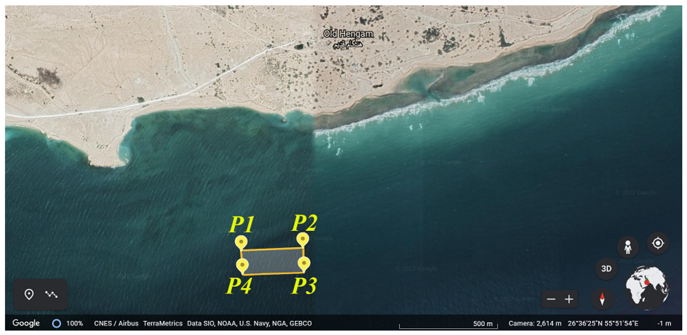
2. Tidal Site Selection

In this section, a tidal site is selected in the southern waters of Iran to illustrate the benefits and the applicability of the proposed methodology. This site’s geometry and flow field are idealized and numerically modeled to examine its potential for implementation of the first pilot tidal stream energy farm in Iran. Several factors are influencing the proper selection of a tidal farm location. As reflected in [1], for efficient utilization of ocean space, shortening the submarine cable length, and lowering the difficulty of tidal power farm construction, it is preferable to build a tidal farm with the minimum employed area. Besides, there are also other important parameters for the selection of a permitted tidal farm in the prescribed region (i.e., southern waters of Iran):

• Small pilot farms are preferred because of the availability of giant oil and gas resources in this part of Iran and the need for significant capital investment on the tidal energy projects.
• Existence of fragile marine life and habitat in this site leads to environmental issues for the development of large tidal farms in this site. Again small pilot farms are preferred.
• Minor variations of bathymetry in this site [1]. This will significantly decrease computational time and cost. Furthermore, it smoothens the pathway for idealizing the geometry and the flow field within site.

According to these discussions, and based on a previous study of Radfar et al. [1], a pilot site is selected with the dimensions of 280 [m] by 130 [m] and a constant depth of 30 [m]. Figure 1 shows the location of the corners of the selected tidal site in the south of Hengam Island in Iran. The dimensions of this site are 280 [m] by 130 [m], with a constant depth of 30 [m]. The latitudes and longitudes of the corners are presented in

Table 1. Geographical coordinates of the selected tidal farm.

Corner ID	Latitude (deg)	Longitude (deg)
P1	26.6072	55.8700
P2	26.6072	55.8728
P3	26.6060	55.8728
P4	26.6060	55.8700

.

As can be seen, the selected tidal site geometry is idealized to have the shape of a rectangular cube with the previously mentioned dimensions (see Section 2) and a constant depth as shown in Figure 2. It is more straightforward to present farm dimensions based on the diameter of rotors.

All simulations of this paper are based on DOE Reference Model 1 (DOE RM1) turbine model. The US Department of Energy (DOE), in collaboration with the National Renewable Energy Laboratory (NREL), proposed this device as an open-source design for horizontal axis hydrokinetic turbine (HAHT), and researchers can use this to benchmark their studies [19]. Since the nominal diameter of DOE RM1 is 20 m, the dimensions of the permitted tidal channel are 14D × 6.5D × 1.5D. It should be noted that HAHTs mechanism for extracting energy from tidal streams in much the same as the mechanism by which wind turbines extract energy from wind [20]. Therefore, an interesting future research direction would be applying the current methodology for wind farms. In this respect, previous studies have proven the great potential of wind energy exploitation in the southern coasts of Iran. An overview of the related literature is provided in [21].

3. Numerical Model

In the present study, the fluid mechanics of the channel is modeled by solving the RANS equation closed by k-$\omega$ turbulent model. the operation of turbines within the modeled farm is simulated via BEM coupled with RANS. This section provides a brief description of numerical modeling.

3.1. Turbine Modeling: BEM

As mentioned before, BEM is used to simulate the operation of turbines in the tidal farm numerically. In BEM, turbine blade span is divided into small elements from root to tip. Here, elemental lift and drag forces are computed based on local flow field velocity, computed as a solution to the RANS equations, and provided lookup table of lift and drag coefficients as a function of Angle of Attack (AOA) for each element. The dynamic effect of blade rotation is simulated based on time-averaged body forces over a thin full disk with an area equal to the swept area of the turbine, over a full revolution of blades [10]. Final time-averaged body forces have the same magnitude but different signs of the lift and drag forces acting on each segment. This exclusion of the actual geometry of blades from numerical modeling of the turbine blades reduces computational costs even up to 100 times while providing an accurate effect of the turbine far wake and turbine-turbine wake interaction [7,22,23,24,25]. This makes the BEM a promising numerical method for the current work.

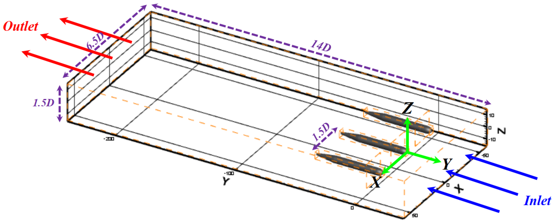
3.2. Model Setup and Boundary Conditions

The imposed boundary conditions are uniform streamwise velocity with a magnitude of 1.75 m/s (this velocity is based on the real tidal stream velocity of the selected farm based on the previous study [1]) and atmospheric pressure at inlet and outlet, respectively. The other boundaries of the computational domain are modeled as slip-free walls. BEM discretization has about 3.86 × ${10}^6$ elements. The number of nodes on the length, width and depth of the domain is 338, 127, and 29, respectively. Mesh is structured in most of the computational domain except for the regions close to the nacelles. For the sake of achieving mesh independency, the mesh resolution near the rotor zone and nacelles was changed in seven steps to obtain the desired mesh accuracy in power estimation of rotors. Attention should be paid to the meshing of the rotor zone. The rotor zone is a thin volume just upstream of the rotor face. Duplicate faces must be avoided here. Besides, the mesh must have a full 360 unit circular face as the rotor face. This paper uses Spallart-Allmaras or SST $\kappa -\omega$ as the turbulent model. Also, discretization of gradient, pressure and momentum for modeling the flow field around turbine blades are “Green-Gauss Node Based”, “Second-Order”, and “QUICK”.

Figure 3 shows the computational domain for a single rotor zone. It is worth mentioning that the farm geometry is constructed by putting together the modules of these single rotors. Fluid zone and nacelle have been specified by gray color. BEM can model different configurations of multiple rotor zones by simply turning them on or off within the computational domain. This feature enables the possibility of different turbine array configurations using a fixed mesh. The boundary conditions are uniform stream-wise velocity and pressure at inlet and outlet, respectively. The outer boundaries of the computational domain are modeled as slip-free walls. The height of the inlet boundary is three blade-radii based on the specifications of the potential site (local depth of 30 m). Also, the length of the rectangular channel is ten blade-radii. In this study, as opposed to similar studies, the actual geometry of the nacelle has been modeled. Also, the outer walls of the nacelle have been modeled as a no-slip condition to capture its effect on wake recovery.

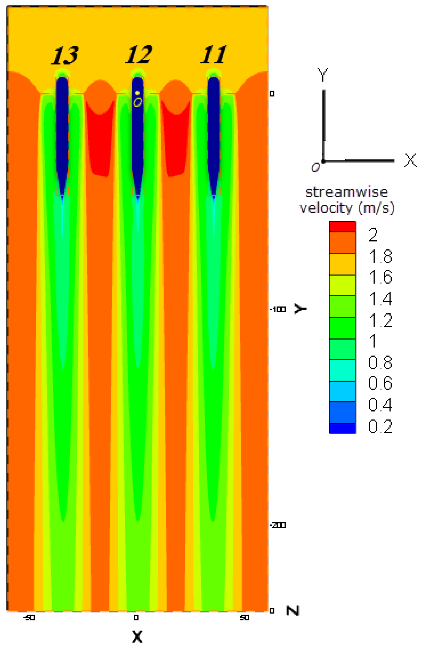
4. Numerical Results

Before discussing the results of numerical simulations, the equation for Available Kinetic Energy flux (AKE) should be defined. AKE can be expressed as [10]:

$$AKE=\frac{1}{2}\rho A{V}^3$$

(1)

where $\rho$ is density of seawater (here, 1025 kg/${\mathrm{m}}^3$) and V is the tidal current speed [m/s]. AKE is calculated based on the area-averaged velocity in a circular surface with the same area that of rotor face:

$$AKE=\frac{1}{A}\sum _{i=1}^n{V}_i\mid A_i\mid$$

(2)

In this section, discussion on the results is based on Normalized Available Kinetic Energy flux (NAKE), which is calculated as:

$$NAKE=\frac{\frac{1}{A}{\displaystyle \sum _{i=1}^n}{V}_i\mid A_i\mid }{\frac{1}{2}\rho A{V}_{\infty }^3}$$

(3)

where $V_{\infty }$ is the uniform streamwise velocity entering the computational domain through the inlet (here, 1.75 m/s).

The two other parameters are global and local efficiencies. The global efficiency ($E_G$) is defined as the power extracted by the turbine in a specific array position, normalized by the power available in the undisturbed flow at the inlet of the channel:

$$E_G=\frac{P_{extracted}}{\frac{1}{2}\rho A{V}_{\infty }^3}$$

(4)

The important aspect of the efficiency in the array optimization process is how much kinetic energy flux is going through a given position (array placement efficiency) and how efficiently each device in the array extracts energy from the available kinetic energy at that position (the turbine “local efficiency”). The local efficiency ($E_L$) is calculated as:

$$E_L=\frac{P_{extracted}}{\frac{1}{2}\rho A{V}_{local}^3}$$

(5)

where $V_{local}$ the velocity averaged on the projection of the rotor swept area on a plane one diameter upstream of the turbine.

Finding an optimum location for the placement of tidal turbines in a farm causes more power output and less depreciation cost for the devices. Although there were several attempts for layout optimization of lab-scaled tidal farms, still steps are to be passed to reach a level where it is possible to implement optimization studies in full scale. However, it is known that powerful systems with several cores and huge computational costs are needed. Having these in mind, the current study is a very early step toward having an optimized full scale tidal farm. As it is mentioned previously, Mozafari [12] developed a general methodology based on the results of 60 different simulations using various turbine configurations. This methodology supports the idea that there is a linear relationship between the power extracted by the turbine and the AKE flux upstream of the device. It was found that all data falls along the same slope, which is equivalent to the local efficiency of all turbines being constant, regardless of their position in the array. Owing to this fact, a new methodology has been proposed in the following section to put aside the dependence on the site specifications and generalize it for various engineering applications in different areas worldwide where potential tidal stream power is considerable. In the following, the methodology for the turbine array optimization process is presented step by step:

First step: Due to natural (farm width) and technical limitations (in this study, the tip-to-tip distance is 1.5R), a maximum of three turbines can be placed at each row. Figure 4 shows the normalized streamwise velocity contour in the middle plane (z = 0). It can be concluded that the streamwise velocity increases nearly two times between two adjacent turbines due to positive interactions of rotating blades. Also, flow accelerates around the middle turbine, and thus its captured power is 2% more than the other two. The extracted power, the kinetic energy at 1D upstream, the local and global efficiencies of all three turbines are summarized in

Table 2. Results of first row simulation for three turbines.

Turbine ID	AKE at 1D Upstream (kW)	Power (kW)	${\mathit{E}}_{\mathit{L}}$ (%)	${\mathit{E}}_{\mathit{G}}$ (%)
11	782.08	326.78	41.82	41.09
12	782.49	332.99	42.56	41.87
13	782.10	327.07	41.78	41.13

.

Second step: As mentioned earlier, due to the presence of the linear relationship between available kinetic energy at 1D upstream and the extracted power, a methodology had been developed for array optimization objectives. The previous methodology proposed by [12] suffers one major problem; they fitted “Y = mX + b” to data, where Y is the extracted power and X is the available kinetic energy flux at 1D upstream. In case X = 0, this equation yields Y = b, which is physically meaningless. Modifications have been made to generalize this methodology to account for real engineering applications and removing site requirements from the provisions, modifications have been made. The new methodology is proposed in the current study: “In BEM, it is possible to fit a linear relationship in the form of Y = mX between the extracted power (Y) and the available kinetic energy flux at 1D upstream (X), where m is the mean local efficiency of first row turbines.” Based on this methodology, a linear relationship to estimate the power of downstream turbines based on the results of Table 2 can be calculated, as

$$P_{BEM}=0.421\times (\frac{1}{2}\rho A{V}^3)$$

(6)

where, A is the rotor disk swept area and V is the local averaged velocity. Flowchart of numerical methodology is presented in Figure 5.

Third step: Now, it is necessary to verify the validity of the proposed methodology. In this regard, a second row must be added to compare simulated power of turbines against the estimated values of proposed linear relationship. In this step, a suitable location for the turbines of the second row must be specified. In choosing this location, paying attention to three issues is of great importance:

• Basically, it is preferred that the turbines be located in a position with maximum kinetic energy flux and thus maximum energy.
• Turbulence effect should not be too destructive to cause damages on rotor blades and other devices.
• A minimum distance between rotors should be adopted to let the biggest marine biota pass safely through rotors.
• Downstream turbines cannot be placed very close to the upstream turbines due to the negative effects of rotating blades. These effects can deteriorate tidal devices and eclipse the efficiency of the turbine.

At first glance, it seems that the best location for the second row is right after the nozzles of the first row. However, this location could not be reported definitely without further investigations on the turbulence effect. Like any other structures and devices, the cyclic load can cause fatigue damage and structural cracks in the long term in tidal turbines. Turbulence is an additional fluctuating velocity component added to the mean velocity. This fluctuating velocity acts as a dynamic load on the turbine with many cycles within a second of time [26]. DNV guideline states that changes in the local flow field and ambient turbulence intensity are expected due to the wakes of upstream turbines. These wake effects imply considerably increased turbulence. This effect may be significant even when the spacing between the tidal turbines in the tidal array is as large as ten rotor diameters (longitudinally). It is reported that the wake effects can even dominate fatigue effects [27]. Since there is no commercial-scale tidal farm globally, due to the same nature of HAHTs and wind turbines, an example of an existing wind farm helps better understand of the trade-off. Benchmarking wake models in Lillgrund offshore wind farm, located about 10 km off the coast of southern Sweden, shows that 3.3D lateral distance and 4.3D longitudinal distance have been implemented to avoid destructive effects of wakes. Therefore, it is expected that such distance should be applied in tidal farms to avoid compact layout and harmful effects of wake on downstream devices [28].

In order to study the performance of the downstream wakes, NAKE flux and Normalised Turbulence Kinetic Energy (NTKE) in different downstream distances are reported in

Table 3. Normalized values of AKE and TKE.

Distance from the First Row	NAKE	NTKE
2D	1.31	0.115
2.5D	1.28	0.110
3D	1.26	0.106
3.5D	1.25	0.103
4D	1.24	0.100
4.5D	1.23	0.098
5D	1.21	0.096

. It is worth mentioning that NAKE corresponds to the amount of the extracted power, and NTKE describes the intensity of the turbulence forces. Results of Table 3 show that moving from 2D to 5D downstream, available kinetic energy flux and turbulence kinetic energy decrease by 7.2 and 16.5 percent, respectively. These findings suggest that there are uncertainties in the selection of the optimized location for the downstream rows. A trade-off should be made between low turbulence effects and high expected power.

Hitherto, the first and second conditions from the three mentioned conditions for selecting the location of the downstream row have been described. Regarding the third issue, the biggest marine mammal in the farm location must be detected. For the selected farm location in this study, the biggest marine mammal is the Black dolphin. For safety passage of this biota, a minimum distance of six meters should be considered between two adjacent turbines. This helps reduce threatening environmental risks.

In Figure 6, seven different lines for placing the corners of downstream turbines are determined. Looking at the contours of streamwise velocity clearly shows that staggered positions (L1, L3, L5, and L7) are desirable due to higher tidal current velocity, and hence, more AKE. Three of these candidates should be selected to place the second-row turbines. According to the first simulation, rotor 13 has more power than rotor 11. Therefore, turbines of the second row are oriented to the left side of the farm. Thus, the corners of the second-row turbines should be placed on the passes L1, L3, and L5. Besides, a minimum distance of 1.5R has been applied between the ends of the nozzles of the first row with the beginning of the nozzles of the second row to avoid the disruptive effects of rotating blades. Figure 7 shows the velocity contours of this simulation. Also, the quantitative results are summarized in

Table 4. Results of the second simulation for six turbines.

Turbine ID	AKE at 1D Upstream (kW)	Extracted Power (kW)	${\mathit{E}}_{\mathit{L}}$ (%)	${\mathit{E}}_{\mathit{G}}$ (%)	Estimated Power Based on Equation (6) (kW)	Difference between Columns 3 and 6 (%)
11	782.08	326.78	41.82	41.09	328.89	−0.64
12	782.49	332.99	42.56	41.87	329.06	−1.18
13	782.10	327.07	41.78	41.13	329.89	−0.56
21	1008.03	417.46	52.49	41.41	423.91	−1.54
22	1008.20	435.19	54.72	43.16	423.98	2.58
23	771.262	318.61	40.06	41.31	324.34	−1.80

. Now a comparison must be made between the estimated power based on Equation (1) and the actual power based on the simulation. Results of the seventh column of Table 4 clearly show that the maximum difference does not exceed 3%.

More validation tests must be performed for a solid conclusion on the viability of the proposed formula of the methodology. To validate the proposed linear relationship (Equation (2)), further simulations have been conducted in 21 different locations downstream of the first row turbines. All these results are summarized in

Table 5. Comparison between actual and estimated power for 21 different downstream locations.

Case	Downstream Distance	Rotor X-Location (*R)	Rotor Y-Location (*R)	Rotor Z-Location (*R)	Extracted Power (kW)	Estimated Power (Equation (6)) (kW)	Difference between Columns 6 and 7 (%)
		0	−10	0	143.29	149.46	−4.13
Coaxial	5D	−3.5	−10	0	142.28	144.95	−1.84
		−3.5	−10	0	142.09	145.54	−2.37
		1	−10	0	312.78	318.30	−1.74
Staggered	5D	−2.5	−10	0	310.50	319.50	−2.82
		4.5	−10	0	295.72	303.91	−2.70
		0	−15	0	165.32	172.77	−4.31
Coaxial	7.5D	−3.5	−15	0	166.01	169.72	−2.18
		−3.5	−15	0	166.36	169.65	−1.95
Staggered	7.5D	−1	−15	0	319.24	313.75	−1.75
		−4.5	−15	0	322.48	304.88	5.77
		2.5	−15	0	315.12	313.70	0.45
		1	−15	0	319.58	313.96	1.79
		−2.5	−15	0	315.43	313.92	0.48
		4.5	−15	0	322.92	304.72	5.77
		0	−20	0	185.95	149.46	−2.66
Coaxial	10D	−3.5	−20	0	194.11	194.67	−0.29
		−3.5	−20	0	194.36	193.99	0.19
		1	−20	0	325.99	311.54	4.64
Staggered	10D	−2.5	−20	0	321.84	310.70	3.58
		4.5	−20	0	326.33	312.76	4.34

. As seen here, the maximum difference is about 6%, which is acceptable and desirable in engineering applications. An interesting observation is that the extracted power from staggered turbines is significantly more than in coaxial cases. This clearly signifies our previous conclusions. The same approach can be applied in any other downstream rows.

It is important to emphasize again that the main limitation of the current research is that with current knowledge and lack of commercial data on structural effects, there will be uncertainties in selecting the best position for downstream turbines and the minimum distance to prevent structural damages. The findings of this research suggest that several questions remain unanswered at present. Further research should be undertaken to investigate the destructive effects of the turbulence forces on the routine operation of elements of the turbines.

5. Discussions and Conclusions

This study set out to develop a numerical methodology, based on a linear relationship, to reduce the computational cost and alleviate the need for mesh and modeling procedures of the downstream rows. The BEM is used to simulate the operation of turbines due to its numerically computational efficiency. In Section 3, a linear relationship between AKE flux at 1D upstream and the expected power of the downstream turbines was fitted, and a step-by-step straightforward numerical methodology has been proposed. This methodology narrows down the wide range of turbine array configurations, reduces the optimization cost and focuses on estimating the best turbine arrangements in a limited number of rows and columns. Decreasing the need for extra simulations is of great importance for any optimization studies in this field and significantly reduces the computational cost.

The main novelty of this linear methodology is its undeniable advantage in engineering applications. A simple linear relationship reduces the efforts for meshing and the numerical modeling of the downstream turbines. Although there will always be a growing need for more turbines to extract the potential tidal energy in the farms, the remarkable value of the methodology would be seen in industrial estimations. In particular, the results of this research showed that the difference between the predicted value and the actual power does not exceed 6%. Therefore, this numerical methodology can attract great attention in practical applications.

References

1. Radfar, S.; Panahi, R.; Javaherchi, T.; Filom, S.; Mazyaki, A.R. A comprehensive insight into tidal stream energy farms in Iran. Renew. Sustain. Energy Rev. 2017, 79, 323–338. [Google Scholar] [CrossRef]
2. Thiébot, J.; Coles, D.; Bennis, A.C.; Guillou, N.; Neill, S.; Guillou, S.; Piggott, M. Numerical modelling of hydrodynamics and tidal energy extraction in the Alderney Race: A review. Philos. Trans. R. Soc. A 2020, 378, 20190498. [Google Scholar] [CrossRef] [PubMed]
3. Harrison, M.; Batten, W.; Myers, L.; Bahaj, A. Comparison between CFD simulations and experiments for predicting the far wake of horizontal axis tidal turbines. IET Renew. Power Gener. 2010, 4, 613–627. [Google Scholar] [CrossRef] [Green Version]
4. Malki, R.; Masters, I.; Williams, A.; Croft, T. The influence of tidal stream turbine spacing on performance. In Proceedings of the 9th European Wave and Tidal Energy Conference (EWTEC), Southampton, UK, 5–9 September 2011; pp. 10–14. [Google Scholar]
5. Edmunds, M.; Malki, R.; Williams, A.; Masters, I.; Croft, T. Aspects of tidal stream turbine modelling in the natural environment using a coupled BEM–CFD model. Int. J. Mar. Energy 2014, 7, 20–42. [Google Scholar] [CrossRef] [Green Version]
6. Tan, J.; Wang, S.; Yuan, P.; Wang, D.; Ji, H. The Energy Capture Efficiency Increased by Choosing the Optimal Layout of Turbines in Tidal Power Farm. In Energy Solutions to Combat Global Warming; Springer: Cham, Switzerland, 2017; pp. 207–226. [Google Scholar]
7. Javaherchi, T.; Antheaume, S.; Aliseda, A. Hierarchical methodology for the numerical simulation of the flow field around and in the wake of horizontal axis wind turbines: Rotating reference frame, blade element method and actuator disk model. Wind Eng. 2014, 38, 181–201. [Google Scholar] [CrossRef]
8. Lombardi, N.; Ordonez-Sanchez, S.; Zanforlin, S.; Johnstone, C. A hybrid BEM-CFD virtual blade model to predict interactions between tidal stream turbines under wave conditions. J. Mar. Sci. Eng. 2020, 8, 969. [Google Scholar] [CrossRef]
9. Zori, L.A.; Rajagopalan, R.G. Navier—Stokes Calculations of Rotor—Airframe Interaction in Forward Flight. J. Am. Helicopter Soc. 1995, 40, 57–67. [Google Scholar] [CrossRef]
10. Mozafari, A.J. Numerical Modeling of Tidal Turbines: Methodology Development and Potential Physical Environmental Effects; University of Washington: Washington, DC, USA, 2010. [Google Scholar]
11. Ruith, M. Unstructured, multiplex rotor source model with thrust and moment trimming-Fluent’s VBM model. In Proceedings of the 23rd AIAA Applied Aerodynamics Conference, Toronto, ON, Canada, 6–9 June 2005; p. 5217. [Google Scholar]
12. Javaherchi Mozafari, A.T. Numerical Investigation of Marine Hydrokinetic Turbines: Methodology Development for Single Turbine and Small Array Simulation, and Application to Flume and Full-Scale Reference Models. Ph.D. Thesis, University of Washington, Washington, DC, USA, 2014. [Google Scholar]
13. Sufian, S.F. Numerical Modelling of Impacts from Horizontal Axis Tidal Turbines; The University of Liverpool: Liverpool, UK, 2016. [Google Scholar]
14. Li, X.; Li, M.; McLelland, S.J.; Jordan, L.B.; Simmons, S.M.; Amoudry, L.O.; Ramirez-Mendoza, R.; Thorne, P.D. Modelling tidal stream turbines in a three-dimensional wave-current fully coupled oceanographic model. Renew. Energy 2017, 114, 297–307. [Google Scholar] [CrossRef] [Green Version]
15. Li, X.; Li, M.; Jordan, L.B.; McLelland, S.; Parsons, D.R.; Amoudry, L.O.; Song, Q.; Comerford, L. Modelling impacts of tidal stream turbines on surface waves. Renew. Energy 2019, 130, 725–734. [Google Scholar] [CrossRef]
16. Attene, F.; Balduzzi, F.; Bianchini, A.; Campobasso, M.S. Using Experimentally Validated Navier-Stokes CFD to Minimize Tidal Stream Turbine Power Losses Due to Wake/Turbine Interactions. Sustainability 2020, 12, 8768. [Google Scholar] [CrossRef]
17. Bianchini, A.; Balduzzi, F.; Gentiluomo, D.; Ferrara, G.; Ferrari, L. Potential of the Virtual Blade Model in the analysis of wind turbine wakes using wind tunnel blind tests. Energy Procedia 2017, 126, 573–580. [Google Scholar] [CrossRef]
18. Naderi, S.; Parvanehmasiha, S.; Torabi, F. Modeling of horizontal axis wind turbine wakes in Horns Rev offshore wind farm using an improved actuator disc model coupled with computational fluid dynamic. Energy Convers. Manag. 2018, 171, 953–968. [Google Scholar] [CrossRef]
19. Lawson, M.J.; Li, Y.; Sale, D.C. Development and verification of a computational fluid dynamics model of a horizontal-axis tidal current turbine. In Proceedings of the International Conference on Offshore Mechanics and Arctic Engineering, Rotterdam, The Netherlands, 19–24 June 2011; Volume 44373, pp. 711–720. [Google Scholar]
20. CTCN. Tidal Energy; Energy Research Centre of the Netherlands (ECN). 2016. Available online: https://www.ctc-n.org/technologies/tidal-energy (accessed on 10 December 2021).
21. Filom, S.; Radfar, S.; Panahi, R.; Amini, E.; Neshat, M. Exploring Wind Energy Potential as a Driver of Sustainable Development in the Southern Coasts of Iran: The Importance of Wind Speed Statistical Distribution Model. Sustainability 2021, 13, 7702. [Google Scholar] [CrossRef]
22. Masters, I.; Williams, A.; Croft, T.N.; Togneri, M.; Edmunds, M.; Zangiabadi, E.; Fairley, I.; Karunarathna, H. A comparison of numerical modelling techniques for tidal stream turbine analysis. Energies 2015, 8, 7833–7853. [Google Scholar] [CrossRef] [Green Version]
23. Li, X. Three-Dimensional Modelling of Tidal Stream Energy Extraction for Impact Assessment; The University of Liverpool: Liverpool, UK, 2016. [Google Scholar]
24. Makridis, A.; Chick, J. Validation of a CFD model of wind turbine wakes with terrain effects. J. Wind. Eng. Ind. Aerodyn. 2013, 123, 12–29. [Google Scholar] [CrossRef]
25. Javaherchi, T.; Stelzenmuller, N.; Aliseda, A. Experimental and numerical analysis of the performance and wake of a scale–model horizontal axis marine hydrokinetic turbine. J. Renew. Sustain. Energy 2017, 9, 044504. [Google Scholar] [CrossRef]
26. Sæterstad, M.L. Dimensioning Loads for a Tidal Turbine. Master’s Thesis, Department of Energy and Process Engineering, NTNU, Trondheim, Norway, 2011. [Google Scholar]
27. DNVGL-ST-0164: Tidal Turbines. Standard, DNV.GL. 2015. Available online: https://www.dnv.com/energy/standards-guidelines/dnv-st-0164-tidal-turbines.html (accessed on 13 November 2021).
28. Hansen, K.S. Benchmarking of Lillgrund offshore wind farm scale wake models. In Proceedings of the EERA DeepWind 2014 Deep Sea Offshore Wind R & D Conference, Trondheim, Norway, 22–24 January 2014. [Google Scholar]
Figure 1. Location of the selected tidal farm in the southern waters of Iran.
Sustainability 14 01664 g001
Figure 2. Layout of the tidal farm including the first row.
Sustainability 14 01664 g002
Figure 3. Schematic view of the computational domain of a single rotor.
Sustainability 14 01664 g003
Figure 4. Velocity field at z = 0 plane for three turbines of the first row.
Sustainability 14 01664 g004
Figure 5. Flowchart of numerical methodology (n ≥ 1).
Sustainability 14 01664 g005
Figure 6. Possible lines for placing the second row turbines.
Sustainability 14 01664 g006
Figure 7. Velocity field at z = 0 plane for six turbines of second simulation.
Sustainability 14 01664 g007