Insights into Efficient Irrigation of Urban Landscapes: Analysis Using Remote Sensing, Parcel Data, Water Use, and Tiered Rates


Abstract
:1. Introduction
2. Methods
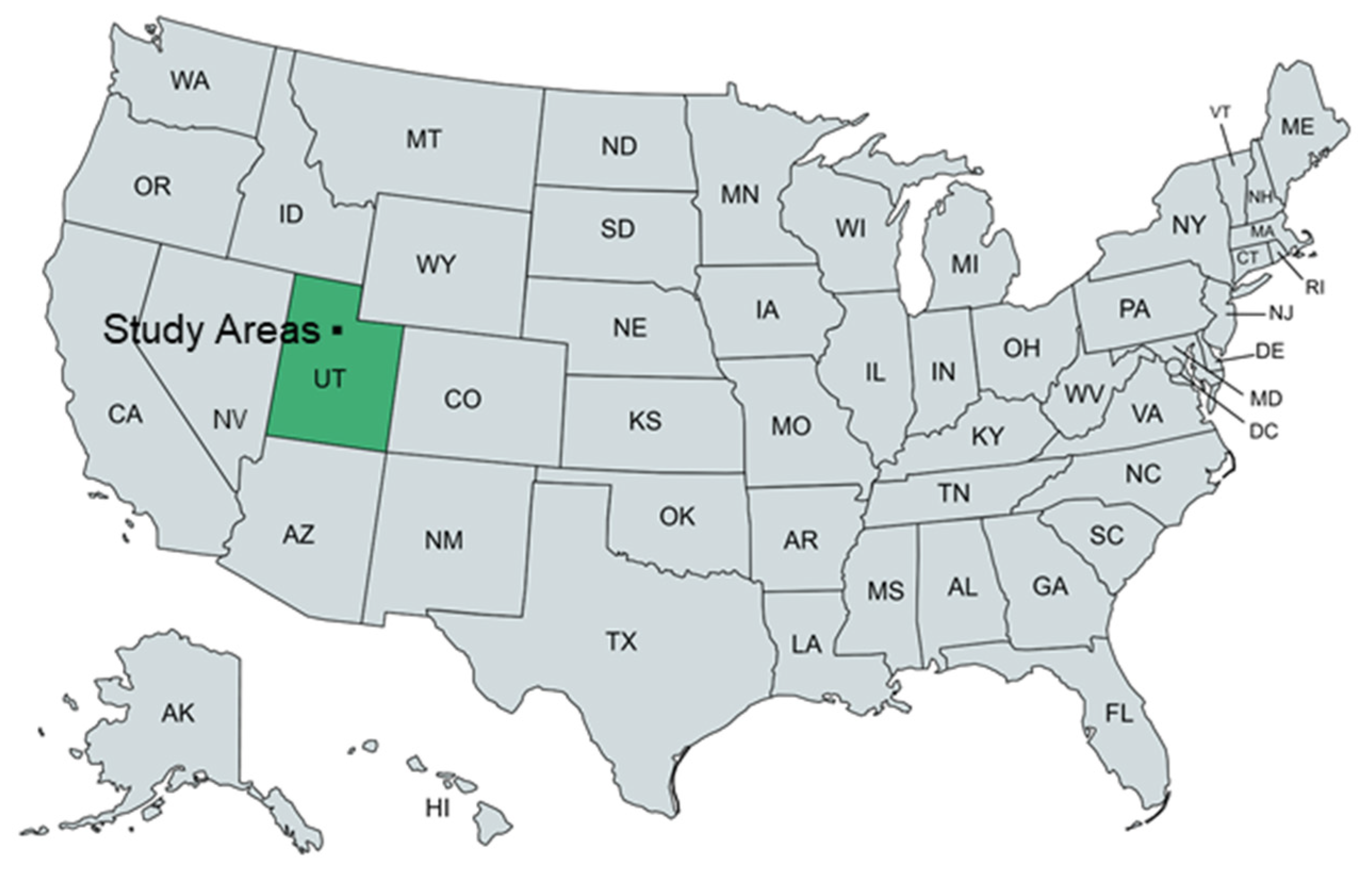
2.1. Study Areas
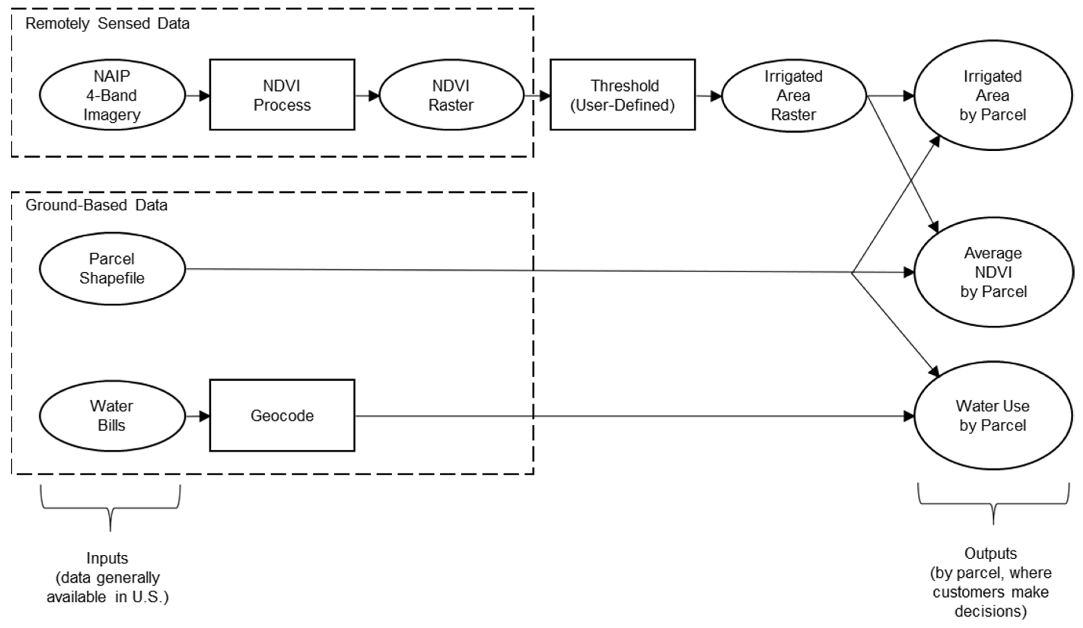
2.2. Data Sources
2.3. Analysis Methods
3. Results and Discussion
4. Conclusions
- Determine the optimum location-specific irrigation depth for best plant health.
- Communicate this optimum value to customers and explain why overwatering is both unnecessary and inadvisable.
- Focus landscape and water conservation programs on proper fertilizer application and other non-water factors that will support healthy lawns and gardens.
- Adjust land-use policies to avoid producing small, irregular, and/or disconnected landscaped areas, especially on small individual parcels. Where green space is needed in high-density developments, encourage larger, contiguous landscaped areas.
- Meter outdoor water use and establish tiered water rates with aggressive tiers that will discourage excessive use.
Supplementary Materials
Author Contributions
Funding
Institutional Review Board Statement
Informed Consent Statement
Data Availability Statement
Acknowledgments
Conflicts of Interest
References
- Dascher, E.D.; Kang, J.; Hustvedt, G. Water Sustainability: Environmental Attitude, Drought Attitude and Motivation. Int. J. Consum. Stud. 2014, 38, 467–474. [Google Scholar] [CrossRef]
- Dettinger, M.; Udall, B.; Georgakakos, A. Western Water and Climate Change. Ecol. Appl. 2015, 25, 2069–2093. [Google Scholar] [CrossRef] [PubMed] [Green Version]
- Gober, P.; Larson, K.L.; Quay, R.; Polsky, C.; Chang, H.; Shandas, V. Why Land Planners and Water Managers Don’t Talk to One Another and Why They Should! Soc. Nat. Resour. 2013, 26, 356–364. [Google Scholar] [CrossRef]
- MacDonald, G.M. Water, Climate Change, and Sustainability in the Southwest. Proc. Natl. Acad. Sci. USA 2010, 107, 21256–21262. [Google Scholar] [CrossRef] [PubMed] [Green Version]
- DeOreo, W.B.; Mayer, P.W.; Dziegielewski, B.; Kiefer, J. Residential End Uses of Water, Version 2; Water Research Foundation: Denver, CO, USA, 2016. [Google Scholar]
- Arshad, J.; Aziz, M.; Al-Huqail, A.A.; Zaman, M.H.u.; Husnain, M.; Rehman, A.U.; Shafiq, M. Implementation of a LoRaWAN Based Smart Agriculture Decision Support System for Optimum Crop Yield. Sustainability 2022, 14, 827. [Google Scholar] [CrossRef]
- Bryld, E. Potentials, Problems, and Policy Implications for Urban Agriculture in Developing Countries. Agric. Hum. Values 2003, 20, 79–86. [Google Scholar] [CrossRef]
- Allon, F.; Sofoulis, Z. Everyday Water: Cultures in Transition. Aust. Geogr. 2006, 37, 45–55. [Google Scholar] [CrossRef]
- Jorgensen, B.; Graymore, M.; O’Toole, K. Household Water Use Behavior: An Integrated Model. J. Environ. Manag. 2009, 91, 227–236. [Google Scholar] [CrossRef]
- Llausàs, A.; Saurí, D. A Research Synthesis and Theoretical Model of Relationships Between Factors Influencing Outdoor Domestic Water Consumption. Soc. Nat. Resour. 2017, 30, 377–392. [Google Scholar] [CrossRef]
- March, H.; Perarnau, J.; Saurí, D. Exploring the Links Between Immigration, Ageing and Domestic Water Consumption: The Case of the Metropolitan Area of Barcelona. Reg. Stud. 2012, 46, 229–244. [Google Scholar] [CrossRef]
- Willis, R.M.; Stewart, R.A.; Panuwatwanich, K.; Williams, P.R.; Hollingsworth, A.L. Quantifying the influence of environmental and water conservation attitudes on household end use water consumption. J. Environ. Manag. 2011, 92, 1996–2009. [Google Scholar] [CrossRef] [PubMed] [Green Version]
- Worthington, A.C.; Hoffman, M. An empirical survey of residential water demand modelling. J. Econ. Surv. 2008, 22, 842–871. [Google Scholar] [CrossRef] [Green Version]
- Sofoulis, Z. Big Water, Everyday Water: A Sociotechnical Perspective. Continuum 2005, 19, 445–463. [Google Scholar] [CrossRef]
- Schindler, S.B. Banning lawns. Georg. Wash. Law Rev. 2013, 82, 394. [Google Scholar]
- Chen, Y.; Zhang, D.; Sun, Y.; Liu, X.; Wang, N.; Savenije, H.H. Water Demand Management: A Case Study of the Heihe River Basin in China. Phys. Chem. Earth Parts A/B/C 2005, 30, 408–419. [Google Scholar] [CrossRef]
- Kenney, D.S.; Goemans, C.; Klein, R.; Lowrey, J.; Reidy, K. Residential Water Demand Management: Lessons from Aurora, Colorado 1. J. Am. Water Resour. Assoc. 2008, 44, 192–207. [Google Scholar] [CrossRef]
- Miller, E.; Buys, L. The Impact of Social Capital on Residential Water-Affecting Behaviors in a Drought-Prone Australian Community. Soc. Nat. Resour. 2008, 21, 244–257. [Google Scholar] [CrossRef] [Green Version]
- Fox, C.; McIntosh, B.S.; Jeffrey, P. Classifying Households for Water Demand Forecasting Using Physical Property Characteristics. Land Use Policy 2009, 26, 558–568. [Google Scholar] [CrossRef]
- Chang, H.; Parandvash, G.H.; Shandas, V. Spatial Variations of Single-Family Residential Water Consumption in Portland, Oregon. Urban Geogr. 2010, 31, 953–972. [Google Scholar] [CrossRef]
- Cook, E.M.; Hall, S.J.; Larson, K.L. Residential Landscapes as Social-Ecological Systems: A Synthesis of Multi-Scalar Interactions Between People and Their Home Environment. Urban Ecosyst. 2012, 15, 19–52. [Google Scholar] [CrossRef]
- Morton, T.; Gold, A.; Sullivan, W. Influence of Overwatering and Fertilization on Nitrogen Losses from Home Lawns. J. Environ. Qual. 1988. [Google Scholar] [CrossRef] [Green Version]
- Clark, W.A.; Finley, J.C. Household Water Conservation Challenges in Blagoevgrad, Bulgaria: A Descriptive Study. Water Int. 2008, 33, 175–188. [Google Scholar] [CrossRef]
- Iglesias, E.; Blanco, M. New Directions in Water Resources Management: The Role of Water Pricing Policies. Water Resour. Res. 2008, 44. [Google Scholar] [CrossRef] [Green Version]
- Barta, R.; Ward, R.; Waskom, R.; Smith, D. Stretching Urban Water Supplies in Colorado; Colorado Water Resources Institute, Special Report No. 13; Colorado State University: Fort Collins, CO, USA, 2004. [Google Scholar]
- Thompson, S.C.; Stoutemyer, K. Water Use as a Commons Dilemma: The Effects of Education that Focuses on Long-Term Consequences and Individual Action. Environ. Behav. 1991, 23, 314–333. [Google Scholar] [CrossRef]
- Nieswiadomy, M.L. Estimating Urban Residential Water Demand: Effects of Price Structure, Conservation, and Education. Water Resour. Res. 1992, 28, 609–615. [Google Scholar] [CrossRef]
- Cotler, H.; Cuevas, M.L.; Landa, R.; Frausto, J.M. Environmental Governance in Urban Watersheds: The Role of Civil Society Organizations in Mexico. Sustainability 2022, 14, 988. [Google Scholar] [CrossRef]
- Hunt, D.V.L.; Shahab, Z. Sustainable Water Use Practices: Understanding and Awareness of Masters Level Students. Sustainability 2021, 13, 10499. [Google Scholar] [CrossRef]
- Vasconcelos, C.; Orion, N. Earth Science Education as a Key Component of Education for Sustainability. Sustainability 2021, 13, 1316. [Google Scholar] [CrossRef]
- Cardenas-Lailhacar, B.; Dukes, M.D.; Miller, G.L. Sensor-Based Automation of Irrigation on Bermudagrass During Dry Weather Conditions. J. Irrig. Drain. Eng. 2010, 136, 184–193. [Google Scholar] [CrossRef] [Green Version]
- Davis, S.; Dukes, M. Methodologies for Successful Implementation of Smart Irrigation Controllers. J. Irrig. Drain. Eng. 2015, 141, 04014055. [Google Scholar] [CrossRef]
- Davis, S.; Dukes, M. Implementing Smart Controllers on Single-Family Homes with Excessive Irrigation. J. Irrig. Drain. Eng. 2015, 141, 04015024. [Google Scholar] [CrossRef]
- Droogers, P.; Bastiaanssen, W. Irrigation Performance using Hydrological and Remote Sensing Modeling. J. Irrig. Drain. Eng. 2002, 128, 11–18. [Google Scholar] [CrossRef]
- Grabow, G.; Ghali, I.; Huffman, R.; Miller, G.; Bowman, D.; Vasanth, A. Water Application Efficiency and Adequacy of ET-based and Soil Moisture–Based Irrigation Controllers for Turfgrass Irrigation. J. Irrig. Drain. Eng. 2013, 139, 113–123. [Google Scholar] [CrossRef]
- Goetz, M.K. Helping Customers Connect Tiered Rates with Actual Water Use. J. Am. Water Work. Assoc. 2013, 105, 64–66. [Google Scholar] [CrossRef]
- Tsur, Y.; Dinar, A. The Relative Efficiency and Implementation Costs of Alternative Methods for Pricing Irrigation Water. World Bank Econ. Rev. 1997, 11, 243–262. [Google Scholar] [CrossRef]
- Rupprecht, C.; Allen, M.M.; Mayer, P. Tucson Examines the Rate Impacts of Increased Water Efficiency and Finds Customer Savings. J. Am. Water Work. Assoc. 2020, 112, 32–39. [Google Scholar] [CrossRef]
- Chesnutt, T.W.; Pekelney, D.; Spacht, J.M. Water Conservation and Efficient Water Rates Produce Lower Water Bills in Los Angeles. J. Am. Water Work. Assoc. 2019, 111, 24–30. [Google Scholar] [CrossRef]
- Kjelgren, R.; Rupp, L.; Kilgren, D. Water Conservation in Urban Landscapes. HortScience 2000, 35, 1037–1040. [Google Scholar] [CrossRef] [Green Version]
- Richter, B.D.; Blount, M.E.; Bottorff, C.; Brooks, H.E.; Demmerle, A.; Gardner, B.L.; Herrmann, H.; Kremer, M.; Kuehn, T.J.; Kulow, E. Assessing the Sustainability of Urban Water Supply Systems. J. Am. Water Work. Assoc. 2018, 110, 40–47. [Google Scholar] [CrossRef] [Green Version]
- Boyer, M.J.; Dukes, M.D.; Duerr, I.; Bliznyuk, N. Water Conservation Benefits of Long-term Residential Irrigation Restrictions in Southwest Florida. J. Am. Water Work. Assoc. 2018, 110, E2–E17. [Google Scholar] [CrossRef]
- Hill, R.; Barker, J.; Lewis, C. Crop and Wetland Consumptive Use and Open Water Surface Evaporation for Utah; Utah State University: Logan, UT, USA, 2011. [Google Scholar]
- UGRC. NAIP. Available online: https://gis.utah.gov/data/aerial-photography/naip/ (accessed on 30 December 2021).
- Abdellatif, M.A.; El Baroudy, A.A.; Arshad, M.; Mahmoud, E.K.; Saleh, A.M.; Moghanm, F.S.; Shaltout, K.H.; Eid, E.M.; Shokr, M.S. A GIS-Based Approach for the Quantitative Assessment of Soil Quality and Sustainable Agriculture. Sustainability 2021, 13, 13438. [Google Scholar] [CrossRef]
- Chakhar, A.; Hernández-López, D.; Ballesteros, R.; Moreno, M.A. Improvement of the Soil Moisture Retrieval Procedure Based on the Integration of UAV Photogrammetry and Satellite Remote Sensing Information. Remote Sens. 2021, 13, 4968. [Google Scholar] [CrossRef]
- Pereira, F.C.; Smith, C.; Maxwell, T.M.; Charters, S.M.; Logan, C.M.; Donovan, M.; Jayathunga, S.; Gregorini, P. Applying Spatial Analysis to Create Modern Rich Pictures for Grassland Health Analysis. Sustainability 2021, 13, 11535. [Google Scholar] [CrossRef]
- Tucker, C.J.; Choudhury, B.J. Satellite Remote Sensing of Drought Conditions. Remote Sens. Environ. 1987, 23, 243–251. [Google Scholar] [CrossRef]
- Peters, A.J.; Walter-Shea, E.A.; Ji, L.; Vina, A.; Hayes, M.; Svoboda, M.D. Drought Monitoring with NDVI-Based Standardized Vegetation Index. Photogramm. Eng. Remote Sens. 2002, 68, 71–75. [Google Scholar]
- Ji, L.; Peters, A.J. Assessing Vegetation Response to Drought in the Northern Great Plains Using Vegetation and Drought Indices. Remote Sens. Environ. 2003, 87, 85–98. [Google Scholar] [CrossRef]
- Karnieli, A.; Agam, N.; Pinker, R.T.; Anderson, M.; Imhoff, M.L.; Gutman, G.G.; Panov, N.; Goldberg, A. Use of NDVI and Land Surface Temperature for Drought Assessment: Merits and Limitations. J. Clim. 2010, 23, 618–633. [Google Scholar] [CrossRef]
- Myneni, R.B.; Hall, F.G.; Sellers, P.J.; Marshak, A.L. The Interpretation of Spectral Vegetation Indexes. IEEE Trans. Geosci. Remote Sens. 1995, 33, 481–486. [Google Scholar] [CrossRef]
- Hashim, H.; Abd Latif, Z.; Adnan, N.A. Urban Vegetation Classification with NDVI Thresold Value Method with Very High Resolution (VHR) PLEIADES Imagery. Int. Arch. Photogramm. Remote Sens. Spat. Inf. Sci. 2019, XLII-4/W16, 237–240. [Google Scholar] [CrossRef] [Green Version]
- Shedd, M.; Dukes, M.D.; Miller, G.L. Evaluation of Evapotranspiration and Soil Moisture-Based Irrigation Control on Turfgrass. In Proceedings of the World Environmental and Water Resources Congress 2007: Restoring Our Natural Habitat, Tampa, FL, USA, 15–19 May 2007; pp. 1–21. [Google Scholar]
- Clay, D.E.; Kharel, T.P.; Reese, C.; Beck, D.; Carlson, C.G.; Clay, S.A.; Reicks, G. Winter Wheat Crop Reflectance and Nitrogen Sufficiency Index Values are Influenced by Nitrogen and Water Stress. Agron. J. 2012, 104, 1612–1617. [Google Scholar] [CrossRef] [Green Version]


| Characteristic | Study Area A | Study Area B |
|---|---|---|
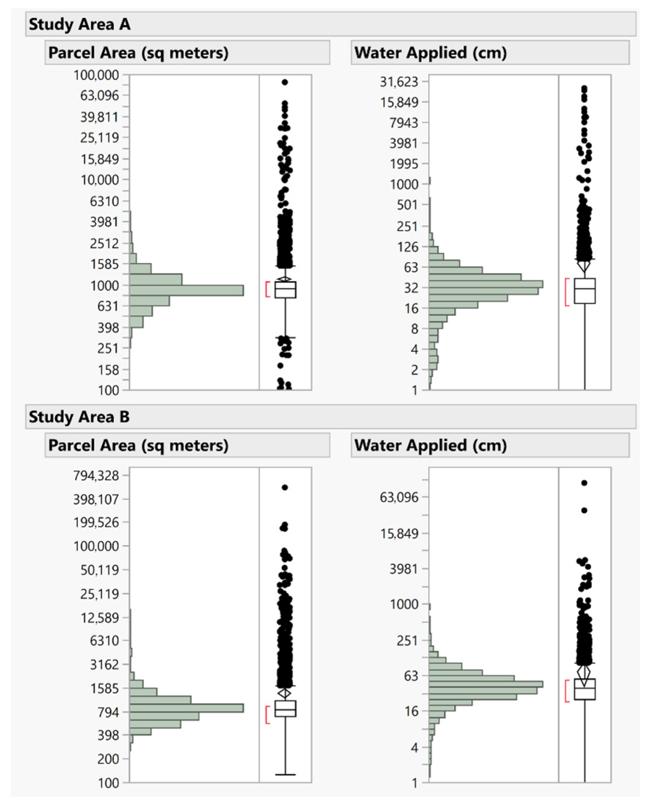
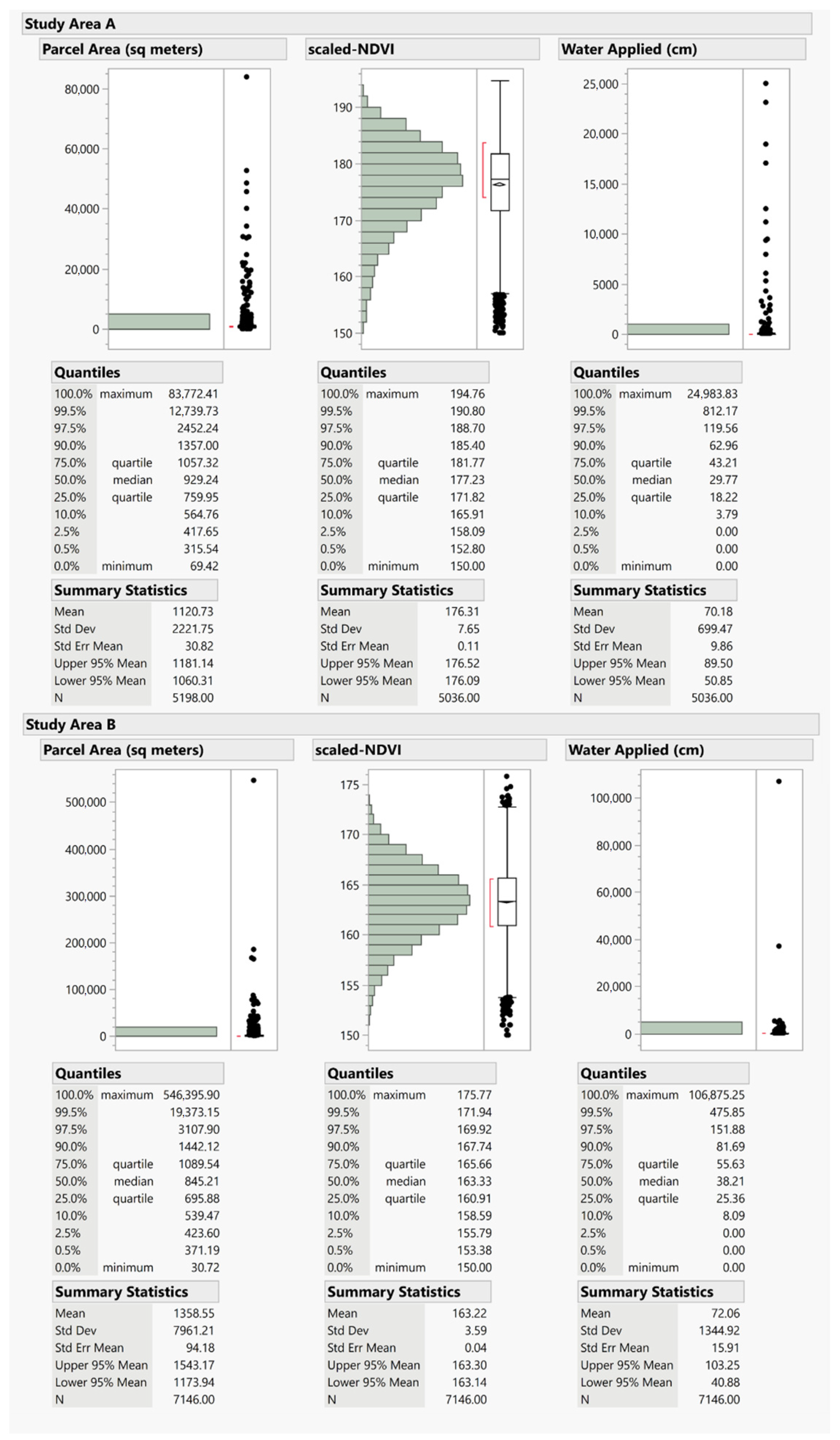
| Irrigation connections | 5198 | 7146 |
| Total irrigated area, ha | 244 | 328 |
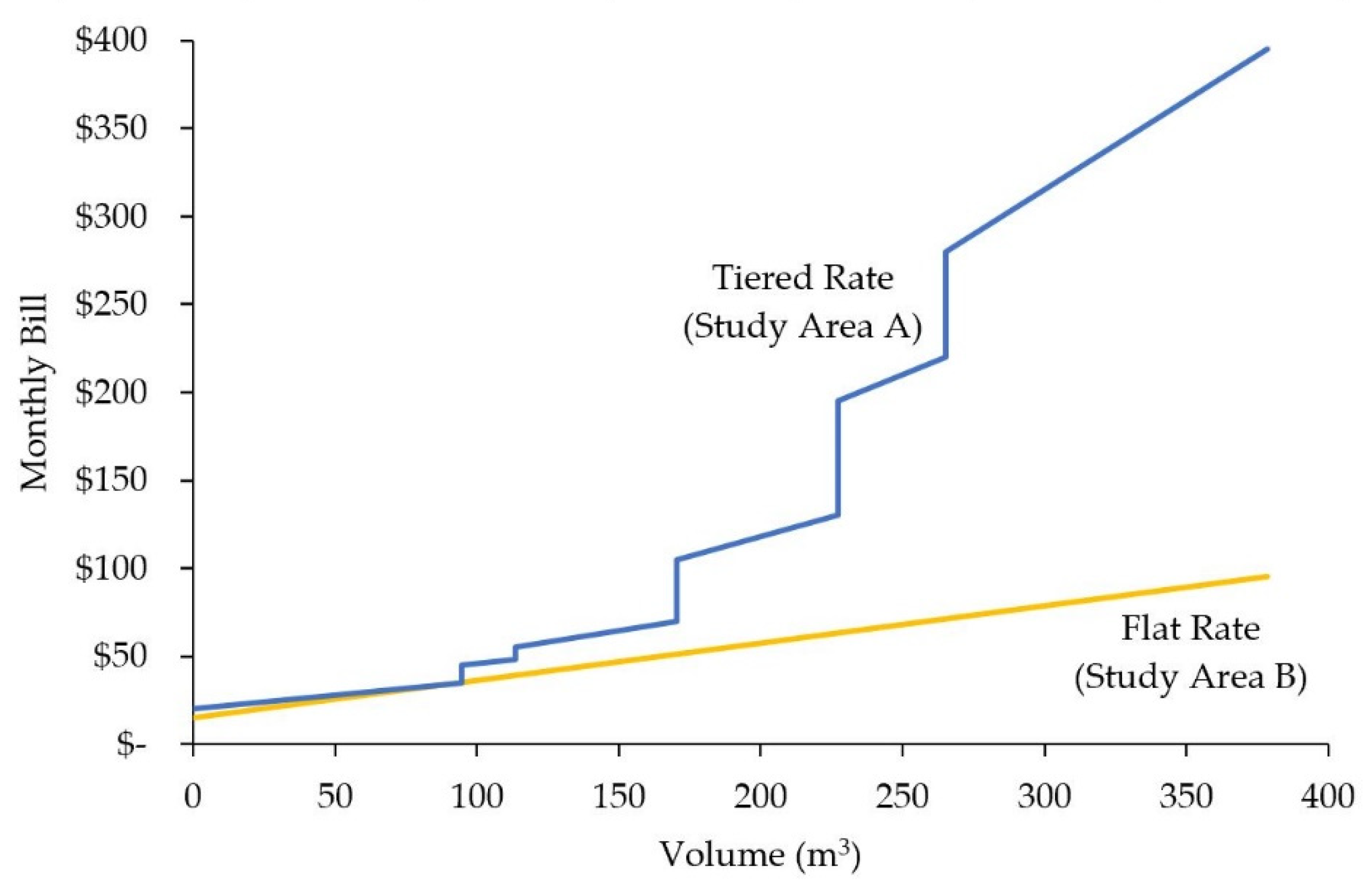
| Rate structure (Figure 2) | Tiered | Flat |
| Annual average precipitation, cm 1 | 32.3 | 53.6 |
| Annual evapotranspiration, cm 1 | 135 | 131 |
Publisher’s Note: MDPI stays neutral with regard to jurisdictional claims in published maps and institutional affiliations. |
© 2022 by the authors. Licensee MDPI, Basel, Switzerland. This article is an open access article distributed under the terms and conditions of the Creative Commons Attribution (CC BY) license (https://creativecommons.org/licenses/by/4.0/).
Share and Cite
Shurtz, K.M.; Dicataldo, E.; Sowby, R.B.; Williams, G.P. Insights into Efficient Irrigation of Urban Landscapes: Analysis Using Remote Sensing, Parcel Data, Water Use, and Tiered Rates. Sustainability 2022, 14, 1427. https://doi.org/10.3390/su14031427
Shurtz KM, Dicataldo E, Sowby RB, Williams GP. Insights into Efficient Irrigation of Urban Landscapes: Analysis Using Remote Sensing, Parcel Data, Water Use, and Tiered Rates. Sustainability. 2022; 14(3):1427. https://doi.org/10.3390/su14031427
Chicago/Turabian StyleShurtz, Kayson M., Emily Dicataldo, Robert B. Sowby, and Gustavious P. Williams. 2022. "Insights into Efficient Irrigation of Urban Landscapes: Analysis Using Remote Sensing, Parcel Data, Water Use, and Tiered Rates" Sustainability 14, no. 3: 1427. https://doi.org/10.3390/su14031427
APA StyleShurtz, K. M., Dicataldo, E., Sowby, R. B., & Williams, G. P. (2022). Insights into Efficient Irrigation of Urban Landscapes: Analysis Using Remote Sensing, Parcel Data, Water Use, and Tiered Rates. Sustainability, 14(3), 1427. https://doi.org/10.3390/su14031427