1. Introduction
In the early stage of the COVID-19 pandemic, major predictions expected recession of international trade. However, the result was totally different. As the social distancing and lockdown increased the needs for electronic shipping, this resulted in the huge increase in the demand for freight services. Now, the world is experiencing the shortage of shipping capacity and the surge in freight rates [
1]. Hence, improving the efficiency of the supply chain network for global freight companies is gaining more attention than ever for a sustainable international trade system.
Global freight companies perform various functional aspects of logistics including documentation, packing, loading/unloading, transportation, etc. A single company can also have a quite complicated global supply chain network including warehouse, distributors, carriers, forwarders, and shippers [
2,
3]. Due to its international nature, the global network is typically connected with many countries. The markets of each country are also non-identical as they are different in terms of culture, law, regulation, language, economy, etc. Therefore, global freight companies usually operate separate local sales offices for each country, to promptly respond to their different demands with respect to the changes in that region.
In this paper, we focus on the relationship between the Headquarters (HQ) and the local sales offices of a global freight company. The main role of the freight company is assumed to be a carrier who delivers the freights by utilizing its own cargo vehicles such as truck, ship, aircraft, etc. Between the company and the shippers, as there are forwarders who collect and aggregate the shipment, the local sales office mainly deals with the forwarders in the region. The local sales offices provide efficiencies in controlling the booking requests and building relationships with local forwarders who are the main customers of the company [
4]. The main role of the local sales office is assumed as generating demand by utilizing sales effort. At some point of time before departure, a portion of cargo space from location to location is sold in advance via a long-term contract and the rest is sold by spot sales. Before the local sales offices decide the level of their efforts, they are informed of the size of the allocated cargo space they can sell.
The local sales offices act as decentralized agents because it is hard for the HQ to exactly control and monitor their decisions on effort levels for long-term and spot sales. The only way for the HQ to control the behaviour of the local sales offices is to change the allocation of the cargo space that they can utilize. After the allocation is determined by the HQ, the local sales offices try to maximize their own profit by making an optimal decision on effort levels. As the total revenue generated by the local sales offices decides the performance of the entire firm, controlling the local sales offices is a critical issue for the company.
Allocation is one of the widely used mechanisms to improve the efficiency of a supply chain when the demand from the buyers exceeds the limited capacity of the supplier [
5]. For many firms, it is quite difficult to increase the capacity without spending significant amount of cost and time in industries such as steel, semi-conductor, airline, etc. Therefore, various types of allocation methods are utilized by those firms [
6,
7,
8]. It is also difficult for the global freight companies to expand the capacity of carriers in a short time, and it is almost impossible for them to control the local sales agents who want to maximize their local profits, due to regional and time constraints. In this situation, the capacity allocation method should be one of the ways for the company to manipulate the behaviour of the local agents.
In this paper, we investigate three different allocation methods: decentralization, centralization, and mixed. In the decentralization method, the HQ of the company allocates the total space of the carriers to the local sales offices before departure, and then the assigned amount of capacity is ensured. Hence, even if one local sales office ends up not fully utilizing the resource of a cargo vehicle, the remaining capacity is not to be assigned to any other local offices if possible. Based on the size of the allocated space, the sales office decides its optimal effort level to maximize its own profit while the HQ aims to maximize the profit on the firm level. Therefore, this method could be less profitable than the centralized control by the company assuming it has full information. In the centralization method, while the HQ does not allocate to each local sales office, the space is fully controlled by the HQ. The local sales office has to compete for the total capacity and the more expensive freight wins priority. Mixed method is a combination of the decentralization and centralization method. Before allocating independent space to each sales office, the HQ retains some space as a buffer for common use. In other words, there can be a portion of the total space capacity that is not assigned to any local sales office. After filling up their assigned space, the freights from each region begin to fill the retained common capacity. In this stage, the HQ has full control over this retained capacity, similar to the centralization method, and the acceptance/rejection of shipment orders is purely based on profitability. This condition thereby draws our fundamental questions:
In one local region, what is the optimal allocation of cargo space between long-term contract and spot sales?
How should the uncertainty in demand and price be balanced when allocating capacity?
If the local regions are heterogeneous in terms of uncertainty in demand and price, what is the optimal allocation to the sales agents?
Is decentralized management of the sales agent always dominated by centralized management?
If we employ the mixed method combining centralized and decentralized management, what is the optimal ratio?
In this paper, the global freight company’s problem is to allocate its capacity efficiently, where the capacity means the space of the cargo vehicle. Capacity allocation has been studied by researchers in a wide range of fields including supply chain, revenue management, economics, etc. To scrutinize the nature of the problem, many studies in supply chain management simplify the problem as having one supplier and two buyers. Cachon and Lariviere [
5] studied three capacity allocation methods: linear, proportional, and uniform, and found conditions where Nash Equilibrium can be formed. Chen et al. [
9] studied two allocation mechanisms: proportional and lexicographic. In the model of one supplier and two retailers, lexicographic allocation can generate more profit for the supply chain. Cho and Tang [
10] compared the uniform and competitive allocation with symmetric retailers. When there is a competition, uniform allocation fails to eliminate the gaming effect and the exact condition for optimization was provided. In this paper, we also adapt the setting of one supplier and two retailers. In the revenue management literature, the capacity allocation problem was studied, where capacity means cargo space. Kasilingam [
11] proposed a simple bucket allocation problem. By modelling inter-program, total contribution was found based on route and flights. In the literature of revenue management, different types of demand are studied: long-term and short-term. Becker and Dill [
12] studied a capacity segmentation problem where the segmentation consists of allocated and non-allocated capacity. In this model, the demand from long-term contracts is allocated in advance and then spot sales is assigned later to the non-allocated capacity. Chew et al. [
13] studied the allocation of spot sales based on the given amount of long-term contracted space. Their problem concerns the forwarders’ decision making and balances the late delivery cost and opportunity cost. Amaruchkul and Lorchirachoonkul [
14] investigated the allocation problem of a single air-cargo carrier to multiple forwarders. They suggested heuristic solutions for the allocation and the increased benefit can be more than 3 percent.
We also compare the performance of different types of allocation methods: decentralization, centralization, and mixed. Centralization vs. decentralization has been a traditional issue in economics. The principal agent problem is a well-known structure to study the decentralized system. This problem has been studied extensively, which is well summarized by Bolton and Dewatripont [
15]. It is well known in the inventory theory that centralization can provide more profit to the supply chain [
16]. However, there are studies that suggest certain conditions where centralization does not fully dominate decentralization. Channel performance can be lowered in a centralized system when the level of market search is high [
16]. When the markets are different, a higher degree of decentralization can increase the profit of the supply chain [
17]. In the case of a two-echelon supply chain, when the retailer and its competitor face uncertain demand, there could be a contractual arrangement where decentralization performs as well as centralization [
18].
In this paper, our focus is on the inside of the firm. The principal and agent are in the same company. Although each agent maximizes its profit function, the HQ tries to improve the revenue of the entire company. Chang and Harrington [
17] studied the internal supply chain of a retail firm consisting of store managers, and searched for better practices. Ellinger et al. [
19] studied interdepartmental coordination. In particular, they focus on the integration of the marketing and logistic department of a firm. In spite of its importance, traditional literature on the supply chain of the global freight companies mainly focus on the external supply chain and have less attention on the importance of the internal supply chain. Therefore, this paper is one of the first to study the internal supply chain of an international freight firm.
The rest of the paper is organized as follows:
Section 2 describes the problem and the assumptions.
Section 3 analytically investigates the problem of the single agent and suggests a closed-form solution.
Section 4 proposes the model of three allocation methods to two agents: decentralization, centralization, and mixed.
Section 5 provides the results of numerical study. Conclusions are discussed in
Section 6.
2. Problem Description
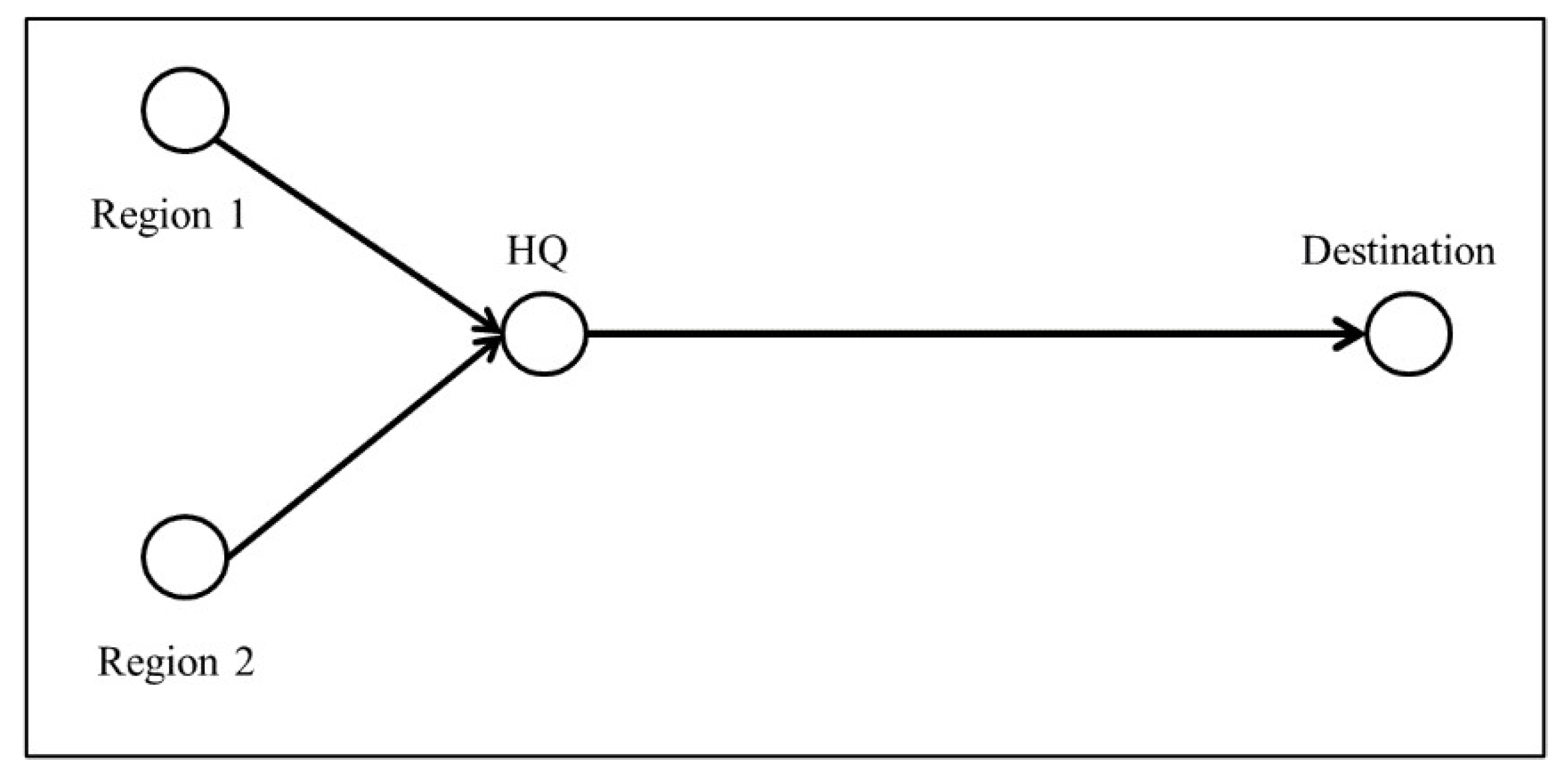
We consider a simple network of a global freight company who operates two sales offices in different regions as shown in
Figure 1. The freights from the two different regions are firstly delivered to HQ where the freights are gathered into one cargo vehicle. Then, the cargo vehicle departs from HQ to the destination. In this paper, as we focus on the delivery between HQ and the destination, the delivery between the two regions to HQ is not considered. We also assume that the operation costs of the two sales offices are the same and fixed.
Our problem has the same structure as a principal-agent problem, and it consists of three decision makers: the HQ and the local sales office 1 and 2. The decision makers are fully rational and risk neutral expected utility maximizer. As the local sales offices also belong to the company, HQ can be considered as the principal in the problem. The local sales office 1 and 2 are the agents who aim to maximize their own payoff. The setting of two agents and a single principal is adapted by many studies in the field of supply chain coordination [
16,
20,
21]. This structure enables us to scrutinize the decisions made by different types of agents in terms of costs of efforts and prices of freights.
As the freights from each region are transferred by a single carrier to the final destination, there can be competition for the space capacity of the carrier if the sum of the amount of freights from both of the local offices exceeds the total space. To guarantee a certain amount of space for each office, the HQ allocates capacity to each local office in many ways. In other words, the firm utilizes different kinds of capacity allocation methods. Capacity allocation is also one of the main issues for supply chain coordination [
11,
12,
22]. However, as far as we know, this is the first study investigating the allocation method for local offices that belong to the same company.
We consider two types of demands: long-term and spot demands [
14,
23,
24] as shown in
Table 1. Long-term demands mainly come from a contract with forwarders [
4]. Forwarders pay a fixed amount for the capacity; therefore, the price is generally lower but the firm has to insure the capacity. The firm also sells capacity on an ad-hoc basis, which is called spot demand. Spot demand offers a higher price but there is a large level of uncertainty in the amount of the demand. In reality, forwarders bid for long-term demands a month before the departure while spot demand comes a few weeks or days before it [
4]. Nevertheless, the decisions on regional allocation of the company take place even earlier than the long-term bidding, and this requires the company to make a prediction on both long-term demand and spot demand. Therefore, we do not take into consideration the different phases of arrival for each type of demand. Instead, we incorporate the difference of each type of demand by using different levels of uncertainty, at the point of time when the firm decides its regional allocation.
We assume that the prices of each long-term sales and spot sales are single and exogenous, and each region is fully separated so the demands are independent. We denote and the unit prices of long-term sales and spot sales at region respectively. Without loss of generality, we assume that the price of spot sales for local office 1 is higher than local office 2, i.e., . To cancel out the case where the firm only accepts long-term demand, we only consider the situation where the summation of the maximum long-term demands from local office 1 and 2 is always less than the total capacity.
As mentioned earlier, each local office exerts effort to utilize demands. We assume that the local offices can put different types of efforts to each long-term and spot demand. Once the allocation is made, each local office decides its own effort levels,
and
, to utilize long-term and spot demand, respectively. The effort level for spot demand,
, determines the probability density function of the random spot demand,
. In addition, the probability density function,
, is a stochastically non-decreasing function of the effort level,
[
25]. The long-term demand,
, is a deterministic and increasing function of the effort level,
. We assume that the cost
is a quadratic function of the effort levels,
.
Typically, three different types of capacity allocation methods can be used by the firm: decentralization, centralization, and mixed. The decentralization method is to allocate the total capacity,
K, to local offices. After the allocation, the freight from each region can only fill its own allocated capacity. We denote the allocation to each office
i as
. Then, after allocation, there is no competition for the space. Next, centralization is the opposite of decentralization because it actually does not allocate any space to the local offices. All the local offices compete with each other over the entire space. When there is competition over the space, the HQ accepts demand based on the priority rule. First, the long-term demand has priority over the spot demand. Second, if the type of demand is the same, the one with the higher price has more priority. The mixed method is a combination of decentralization and centralization. The firm firstly allocates some space to each office. Then, the firm retains the part that is not allocated to any office, as common space. We denote this retained common space as
. Throughout the paper, we use the notations that are summarized in
Table 2.
3. Optimal Effort Levels in a Single Office
In this section, we consider the optimal decision on effort levels for both the long-term and spot sales in a single office. We first develop a mathematical model to determine optimal effort levels for a single office. As we are considering the problem of a specific office
i, we use notations without the subscript
i as shown in
Table 2. We also use the notation
to denote
. We assume that the effort levels,
, are put into long-term and spot sales, respectively. As the amount for long-term demand must be allocated first, the available capacity for long-term demand is equal to
. On the other hand, the remaining capacity for spot sales is
. Therefore, the total revenue for a single office is expressed as follows.
Now, let
be a cost function for the effort levels
. We also use the notation
to denote mathematical expectation. Then, the optimal effort levels are determined by solving the following optimization problem to maximize the expectation of the total profit,
, as follows. The notation
denotes “subject to”.
Similar to the assumption in [
26,
27,
28,
29], we assume that the cost function,
, for the effort levels,
, is quadratic as follows.
On the one hand, we assume that there is no uncertainty in the amount of long-term sales, similar to Chew et al. [
13]. For the effort level
, the long-term demand,
, is assumed to be a deterministic linear function defined by
. On the other hand, the spot demand,
, is assumed to be random. Similar to the work of He et al. [
25] and Taylor [
30], we also assume that the effort affects demand in an additive form, i.e.,
. For the simplicity of analysis, we consider the case where
follows the uniform distribution,
. As
, we obtain that
.
Under the above assumptions, the total profit,
, in problem (
2) for a single office is expressed as follows.
In order to eliminate trivial cases, we assume that
. As
and
, we can simplify the above Equation (
3) as follows.
As the decision on long-term sales is always prior to the one on spot sales, the following optimization problem should be solved for a given
. Let
. Then,
Proposition 1. For a given , function is defined in a closed form as follows. Proof of Proposition 1. To simplify , we divide the interval of into the following three cases.
(Case 1) .
As
, we have
. Hence,
. Then,
in problem (
5) is obtained as follows.
(Case 2) .
If
, then
. Thus,
. Otherwise,
. Then,
in problem (
5) is obtained as follows.
(Case 3) .
As
, it is trivial that
. Hence,
. Then,
in problem (
5) is obtained as follows.
which completes the proof. □
Using the result of Proposition 1, we find an optimal solution for the effort level of spot sales, , as stated in Theorem 1.
Theorem 1. Assume that . For a given , an optimal solution, , of the problem (5) is obtained as follows. - (i)
If , then .
- (ii)
If , then .
Proof of Theorem 1. First, we give a proof for the condition (i)
. If we consider (case 1)
, then we have
To find out an optimal solution,
, maximizing
, we take a derivative with respect to
and set it equal to 0. Then, we obtain
From the condition (i)
, an optimal solution for (case 1) is obtained as
.
If we consider (case 2)
, then we have
To find out an optimal solution,
, maximizing
, we take a derivative with respect to
and set it equal to 0. Then, we obtain
As
, it is clear that
. Thus, an optimal solution in (case 2) is obtained as
.
Finally, if we consider (case 3)
, then we have
To maximize
in (case 3), an optimal solution is obtained as
. Now, as
, we conclude that
.
The proof for the condition (ii) is almost identical except for the following details. First, for (case (ii)-1), . Second, for (case (ii)-2), . Finally, as , we see that and . Therefore, we conclude that . □
In Theorem 1, we see that the optimal effort level for spot sales,
, is affected by the effort level for long-term sales,
. Now, we try to find an optimal effort level for long-term demand,
. Let
be given as the result of Theorem 1. Let
. Then, in order to find an optimal solution,
, we have to solve the following optimization problem.
Proposition 2. Function is defined in a closed form as follows. Proof of Proposition 2. First, we consider the case (a)
. By using the result of Theorem 1, we obtain that
. As
, we obtain
as follows.
Now, using
, we simplify
as follows.
Next, we consider the case (b)
. By using the result of Theorem 1, we see that
. As
, we also note that
. Thus, we obtain
as follows.
Now, using
, we simplify
as follows.
which completes the proof. □
Using the result of Proposition 1, we obtain an optimal solution for the effort level of long-term sales, , as stated in Theorem 2.
Theorem 2. Define and for simplifying numerical expressions. An optimal solution, , of the problem (6) is obtained as follows. - (i)
If , then .
- (ii)
If , then .
- (iii)
If , then .
- (iv)
If , then
Proof of Theorem 2. We first give a proof for the condition
. If we consider the case (a)
, then we have
To find out an optimal solution,
, maximizing
, we take a derivative with respect to
and set it equal to 0. Then, we obtain
As
, an optimal solution for case (a) is obtained as
.
Next, if we consider the case (b)
, then we have
To find out an optimal solution,
, maximizing
, we take a derivative with respect to
and set it equal to 0. Then, we obtain
As
, an optimal solution for case (b) is obtained as
. Now, as
, we conclude that
.
Second, we prove for the condition . If we consider the case (a) , then as , an optimal solution for case (a) is obtained as . Next, if we consider the case (b) , then as , an optimal solution for case (b) is obtained as . Now, as , we conclude that .
Third, we prove for the condition . If we consider the case (a) , then as , an optimal solution for case (a) is obtained as . Next, if we consider the case (b) , then as , an optimal solution for case (b) is obtained as . Therefore, we conclude that .
Finally, we prove for the condition . If we consider the case (a) , then as , an optimal solution for case (a) is obtained as . Next, if we consider the case (b) , then as , an optimal solution in case (b) is obtained as . Now, we compare which one of the values, and , is larger. If , then we obtain an optimal solution as . Otherwise, an optimal solution is obtained as . □
4. Three Types of Capacity Allocation Methods
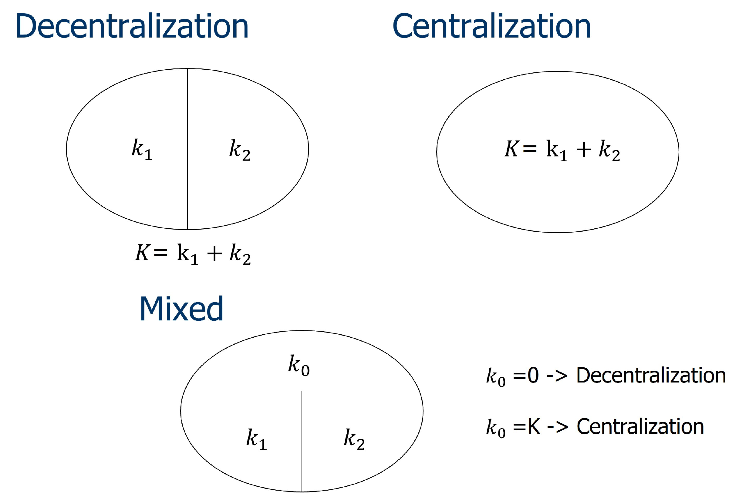
In this section, we investigate three different types of allocation: decentralization, centralization, and mixed. In other words, different levels of decentralization are studied. In the decentralization method, full level of decentralization is given, while in the centralization method, nothing is given. In the mixed method, a partial level of decentralization is used. Thus, as shown in
Figure 2, if
, then the mixed method is equal to decentralization. In case of
, the mixed method is equal to centralization. As mentioned in
Section 3, the following assumptions still hold in this section.
- (A1)
, for ,
- (A2)
where , for , and
- (A3)
, for .
4.1. Decentralization Method
In the decentralization method, the HQ decides how to divide the total capacity, K, and allocate it to each local sales agent . Let and be the allocated capacity to local office 1 and 2, respectively. We assume that the total capacity must be allocated to either one of the local offices, i.e., , and this assumption holds throughout the paper. As the allocation is secured to local agent 1 and 2, respectively, each office only solves its own problem without considering the decision of the other. Furthermore, the competition for a common space is not needed.
When the capacity,
, is allocated to office
i and effort levels of
and
are executed based on the decentralization method, let
be the total revenue of office
i. Then, under the assumption (A1), we obtain the following.
In order for office
i to maximize its expected profit,
, the following optimization problem should be solved.
Let
be an optimal solution of problem (
7) for office
i. Under the assumptions (A1), (A2), and (A3), note that
can be obtained in terms of Equation (
1). Hence, the optimal effort,
, can be derived using results of Theorems 1 and 2.
Now, for the HQ to maximize its expected revenue
, the optimal allocation
should be obtained by solving the following optimization problem.
4.2. Centralization Method
In the centralization method, as there is no allocation to each local office by the HQ, both offices must compete for the total capacity,
K. When the effort level
is utilized for office
i, let
be the total revenue of office
i. Note that long-term demand is always prioritized over spot demand in the total capacity and the sum of long-term demand does not exceed the total capacity
K. Under the assumption that the price of spot sales for local office 1 is higher than local office 2 (i.e.,
), as mentioned in
Section 2, the problem of local office 1 is similar to that described in the decentralization method. The only difference is that, instead of the allocation,
, the available capacity for local office 1 becomes
. Under the assumption (A1), note that
. Hence, we obtain that
Under the assumption (A3), as office 1 aims to maximize its expected profit,
, the following optimization problem should be considered.
Under the assumptions (A1), (A2), and (A3), note that
can be obtained in terms of Equation (
1) in
Section 3. For a given
, the optimal effort,
, can be derived using results of Theorems 1 and 2. As
and
are functions of the given
, the optimal solutions for problem (
8) are expressed as
and
. For the given
, let
be the available capacity for spot sales at office 2 in the centralization method. Then,
is also a function of
, expressed as follows.
Thus, we have
As office 2 wants to maximize its expected profit,
, the following optimization problem should be considered.
In the centralization method, as the HQ makes no decision on allocation of capacity, the expected revenue of the HQ,
, is given as follows.
4.3. Mixed Method
The mixed method is a hybrid approach obtained by combining decentralization and centralization methods. In the mixed method, the HQ defines a shared portion of the total capacity K as and allocates the remaining capacity to two local offices as and , respectively. Office 1 can use its dedicated capacity, , independently from office 2. Even if there are remaining capacity in , it can not be used by office 2. When the effort level, , are utilized by the office and the amount is allocated to the office by the HQ, let be the revenue of office i.
Under the assumption that the price of spot sales for local office 1 is higher than local office 2 (i.e.,
), as mentioned in
Section 2, the problem of local office 1 is similar to that mentioned in the decentralization method. Note that the available capacity for office 1 is a function of
. Under the assumption (A1), note that
Then, we have
As office 1 wants to maximize its expected profit,
, under assumption (A3), the following optimization problem should be considered.
Under the assumptions (A1), (A2), and (A3), note that
can be obtained in terms of Equation (
1) in
Section 3. For a given
, the optimal effort,
, can be derived using results of Theorems 1 and 2. As
and
are functions of the given
, the optimal solutions for the problem above are expressed as
and
.
When office 2 determines the effort level for spot sales (i.e.,
), it is affected by both the effort levels of office 1,
, and the effort level for its long-term sales (i.e.,
). For the given
, let
be the available capacity for spot sales at office 2. Then,
, is expressed as follows.
Then, the revenue of office 2 is obtained as follows.
As office 2 wants to maximize its expected profit, the following optimization problem should be solved.
Let
be an optimal solution of problem (
9) and (
10) for office
i. For the HQ to maximize its revenue
, the optimal allocation
should be computed by solving the following optimization problem.
5. Computational Study
5.1. Testing Environment
As the behaviour of the two local sales offices are analytically intractable, we numerically evaluate and compare the performance of each allocation method. The numerical test is constructed and implemented by using MATLAB. In the decentralization method, each sales agent chooses its own optimal effort level according to the closed-form solution obtained from Theorem 1 and 2. Therefore, for the maximization of the total revenue of the firm, the optimal allocation to each agent, and , are searched within the total capacity, K.
In the centralization method, each local agent does not simply choose the optimal effort without considering the effort level of the other agent. Hence, we develop a simulation model to evaluate the realized payoff for each agent and find the optimal effort for each local sales agent. Without loss of generality, we assume that region 1 is superior in terms of price for spot sales. In a game-theoretic setting, the first mover should be the local sales office 1 and then the local sales office 2 decides its optimal effort level. The sequence of decisions made in centralization is as follows. First, each local sales office decides the effort for the long-term sales. As we only consider the case when the summation of the maximum long-term demand from each region does not exceed the total capacity, both sales offices can choose the optimal level of effort for the long-term demand. Without loss of generality, we assume that the local sales office 2 chooses the effort level for the long-term demand. As long-term demand has priority, the long-term demand utilized by the effort level will be secured. Then the local sales office 1 decides the optimal effort level for the long-term and spot demand to maximize its own profit. As the price of the spot demand for local office 1 is greater than that of local office 2, local office 2 can search its optimal effort within the remaining space of . As the spot demand from region 2 is not deterministic, the demand will be realized based on its probability distribution function that is assumed to be uniform in this paper. Finally, the remaining space can be obtained by the spot demand from region 2. We also assume that both offices are fully capable of evaluating the expected profit and predicting the optimal effort level of the other within this game-theoretic setting. By expecting the optimal effort level of the local sales office 2 and evaluating the expected payoff, the local sales office 1 finalizes its optimal effort level. Due to the probabilistic nature of the demand, the outcome of the spot demands from both regions are randomly generated and the simulation of the demand is performed through 1000 iterations.
In the mixed method, the optimal effort levels are searched by changing the common space, , and the allocated space and . As we do not have a closed-form solution for this setting, the optimal effort levels of each agent are simulated as follows. First, allocation is given. Then, all of the effort levels are tested and the corresponding profits are computed. The effort levels with the biggest profit are chosen as the local optimal solution based on the given allocation. All of the possible allocations are tested and the allocation with the biggest profit would be the optimal allocation .
5.2. Numerical Results
We consider the research questions raised in
Section 1 by performing numerical studies. First, we check whether one of the centralization or the decentralization method dominates the other. Without loss of generality, by having local sales agent 1 as the focal player, we fix the price and cost of the local sales agent 2. Then, by changing the parameters of the local sales agent 1, we investigate the behaviour of each agent and the performance of the two allocation methods. Then, the revenue at firm level is evaluated for the decentralization method and the centralization method each. The parameters for the two agents are used as shown in
Table 3.
The price of the long-term demand in region 1,
, is changed from
to
by the increment of
where the other parameters are fixed as given in
Table 3. Then, the expected revenue for the firm, the expected revenue for each sales office, and the optimal effort level for each allocation method based on the change of
are obtained as shown in
Table 4.
As shown in
Table 4, we note that the total expected revenue obtained from the centralization method is greater than that from the decentralization method as
becomes smaller. Furthermore, as
becomes larger, it reacts vice versa. The results showing that more revenue can be obtained from the decentralization method controvert the conventional prediction that the centralization method would outperform due to the pooling effect. When
is lower than
, the centralization method generates more revenue from
to
. However, when
becomes greater than
, the decentralization method begins to outperform and generates
more revenue. This can be regarded significant in the context of revenue management.
Observation 1: Neither the centralization nor the decentralization method dominates the other on the whole range of .
We next scrutinize the situation when the decentralization method outperforms the centralization method. Optimal effort levels obtained from each method are summarized in the following
Table 5.
From the result of
Table 5, we see that the revenue obtained from the decentralization method is greater due to the strategic nature of the setting. As
increases, the natural reaction of the local sales office 1 would be to increase the effort level for long-term demand. This results in more allocation to the local sales office 1 in the case of the decentralization method because the demand from region 1 is more profitable, as described in
Table 5. However, in the centralization method, by knowing that the local sales office 1 would increase its effort level for the long-term demand, the local sales office 2 would increase the effort level for its long-term demand as well, because it is the only item that has the priority in securing some level of profit at least. We clearly see that when
is equal to
, the local office 2 increases
and decreases
in the centralization method while the efforts are
in the decentralization method. As a result, this strategic decision of the local sales office 2 lowers the total revenue of the firm in the centralization method.
Observation 2: To ensure its own profit, the agent in the less profitable region may increase the effort level for long-term demand to secure the allocated capacity, and it can result in the loss of total revenue on the firm level.
Now, we consider the mixed method. It is trivial that the profit from the mixed method would (weakly) dominate the other two methods, as it holds the property of both two methods. We try to find the case when the common area (
) is non-zero.
Table 6 shows the parameters that are used for our simulation of the mixed method. Then, our computational results are summarized as shown in
Table 7.
In
Table 7, we see that the decentralization method dominates over the centralization method. Note that the effort level for long-term demand utilized by local office 2 is larger in the centralization method than the decentralization method. As a result, the effort level for the spot demand decreases dramatically from
to
. Finally, both the expected revenue and the total expected revenue are smaller in the centralization method than the decentralization method. However, in the mixed method,
units of cargo space are fully allocated to local office 2. Therefore, there would be a room of freedom for local office 2 to maximize its revenue without considering the competition with local office 1. This results in an increase in the effort level for the spot demand. At the same time, the common space of
is allocated. Hence, this space can be utilized to hedge the risk of the uncertainty of demands and also the competitive nature of this common space can provide a certain level of profitability.
As there are a number of parameters in the mixed method, we do not find clear relationships between the parameters and the optimal allocation,
. Thus, we focus on the trend between the level of uncertainty,
, and the optimal allocation obtained from the mixed method. Our results are provided in
Table 8.
In
Table 8, we set
and use the term
to indicate both
and
. As we increase
, we see that
increases as well. The allocation to the local sales office 1 is decreased and the one to the local sales office 2 is increased. This is because the optimal common space,
, would be mainly utilized by the local sales office 1. The common space will be used for profitability when the amount of demand for local sales office 1 is enough, and for risk hedging when the amount of demand for local sales office 1 is not enough.
Observation 3: In the mixed method, the optimal allocation of the common space, , increases as the level of uncertainty, , increases.
6. Conclusions
Global freight companies assign local sales offices to each country in order to improve the promptness and the efficiency of the supply chain. The local offices respond to customers in the region, run a promotion to generate more demand, and react to any unexpected changes in the region. They closely communicate with the HQ, frequently update the situation related to the local market and carefully implement the allocation made by the HQ. In spite of its importance, the optimal method for controlling the local sales office has not, to date, been fully studied and developed in either practice or academia.
In this paper, we investigated the optimal capacity allocation method for a freight company who operates local sales offices. First, we developed a mathematical model for the optimal decision on effort levels for both long-term and spot sales in a single local sales office. The information being given on the price and the probability distribution of long-term and spot demand, the cost of the efforts to utilize demand, and the allocated space, an optimal effort level for a single local office is derived in a closed-from. Based on the model for a single office, we then investigated the dynamics between two offices. In addition, to provide a fundamental understanding on the capacity allocation method, we studied three types of allocation methods: decentralization, centralization, and mixed. When the problem is extended to two local offices, it became intractable due to its complexity. Hence, we performed a simulation study to compare the performance of three different allocation methods.
Through the simulation study, we first answered the traditional question of whether one of either decentralization or centralization dominates the other. Our simulation results showed that neither one of the methods dominates the other. It is known that centralization usually performs better than decentralization due to the pooling effect. In the centralization method, if one of the offices is not able to fully use its allocated capacity, it is possible for the other office to utilize the unfilled capacity. However, we found out that in our game-theoretic setting, something beyond this can happen. If one of the offices is inferior in terms of price, it would lose priority when there is competition for common space. One of the ways for the inferior office to secure some amount of space is to increase the long-term demand coming from the region by putting in more effort. As long-term demand has priority to spot demand, the profit generated from it will be secured. While this decision would be beneficial for the inferior office, it may be harmful for the entire company because it reduces the company’s profitability in the end. Therefore, when the company faces such a situation, it is rather better to use the decentralization method.
As the mixed method includes the properties of both the decentralization and the centralization method, it is trivial that the mixed method is the best option. Instead, the optimal amount of the common space, , is still the open question in this case. Therefore, we set up a simulation model to find this optimal amount of common space, . As there are rather a number of parameters associated with this optimal allocation, such as price, cost, the uncertainty level of demand, etc., we did not find clear relationships among the parameters and the optimal allocation to each office and common space. Future research would develop a simple model to investigate the optimal decision on common space.


