Abstract
Large seasonal and spatial variabilities in Arctic shipping and its associated emissions are expected in the future, due to continuous sea ice decline. This study collected ship traffic data and the associated emissions of carbon dioxide (CO2), nitrogen oxides (NOx), sulfur dioxide (SO2), particulate matter (PM), and black carbon (BC) along the Northern Sea Route (NSR) in 2013. The aim is to analyze the seasonal and spatial variations in ship traffic and the associated emissions along the NSR. The potential factors for these variations are discussed. The results showed strong seasonal and spatial variations in ship traffic and the associated emissions. In winter and spring, the number of ships and the associated emissions were low and limited to the Barents Sea. In summer, they almost doubled and showed a clear eastward and northward expansion, covering most of the study area and forming trans-Arctic shipping lanes, which remained throughout the autumn. The spatial distribution of emissions was similar to that for ship traffic, showing a decreasing trend from west to east. SO2 and PM peaked one month prior to the others and exhibited relatively high emissions, especially along shipping lanes, which may be linked to the changes in ship and fuel types.
1. Introduction
Arctic shipping is an emerging topic within the maritime transport sector, due to the gradual decline in sea ice and the consequent increase in accessible waters, which has raised the prospect of increasing Arctic shipping and the potential use of new transit routes, such as the Northern Sea Route (NSR) [1]. An increase in the total traveled distance and number of unique ships in the region has already been observed. By 2015, the total distance traveled by ships in the Canadian Arctic had tripled since the 1990s, while the total distance traveled in the International Maritime Organization (IMO) Arctic Polar Code area increased by 75% from 2013 to 2019 [2,3]. From 2010 to 2016, the number of unique vessels increased by 6.6% per year [4]. The growth in Arctic shipping activity is expected to continue in the future, due to the projected continuous sea ice loss [5,6,7,8].
Shipping is an important source of atmospheric emissions. Increased shipping leads to increased emissions. From 2012 to 2018, shipping-related CO2 emissions in the IMO Arctic Polar Code area almost doubled from 923 to 1845 thousand tonnes [9,10]. The contribution of shipping-related emissions to the total emissions also showed an increasing trend. From 2012 to 2018, in global anthropogenic emissions, the share of emissions from global shipping activity increased from 2.76% to 2.89% [11]. Ship-associated emissions have a negative impact on local air quality, environment, and climate, especially in high-traffic areas [11,12,13,14,15,16,17]. Arctic shipping has a significant impact on local air quality [15,18]; however, this is scarcely studied. This is partly due to gaps in knowledge on the unique Arctic environment and partly due to an enhanced focus on long-range transported pollutants relative to local sources [15,19]. Therefore, it is of great importance to study the ship-associated emissions in the Arctic region.
Due to the presence of sea ice, certain Arctic waters are seasonally accessible, which leads to large seasonal variability in ship traffic and ship-associated emissions [1,4,20,21]. With a longer summer season, a shorter winter season, and an increase in accessible waters, shipping-associated emissions are expected to increase in the future. However, there is a certain gap of knowledge regarding the seasonality of shipping and its associated atmospheric emissions [22]. Numerous shipping emissions inventories for the Arctic have been developed, but they mostly focus on inter-annual comparison and the Arctic as a whole [10,12,23,24,25,26,27]. Studies seasonal variations in ship-associated emissions and the environmental impacts for various Arctic regions have been conducted [15,24,27,28], but these studies are scarce [19] and do not include all seasons. Therefore, it is important to investigate the seasonal variability of Arctic shipping and its associated emissions in detail.
The objective of the study is to investigate the seasonal and spatial distribution of shipping activity and the associated atmospheric emission of carbon dioxide (CO2), sulfur dioxide (SO2), nitrogen oxides (NOx), particulate matter (PM), and black carbon (BC) along the NSR in 2013 and the factors for these variations. The implications of these variations are also discussed. This study can be used as a baseline study for future studies, as 2013 was the first year with available continuous Automatic Identification System-based (AIS) ship traffic data provided by the Protection of the Arctic Marine Environment’s (PAME) Arctic Ship Traffic Database (ASTD).
2. The Northern Sea Route (NSR)
In this study, the NSR and surrounding areas are picked as the study area, due to geographical limitations along the Transpolar Sea Route (TSR) and Northwest Passage (NWP), such as sea ice conditions and water depth, and the fact that the NSR is exposed to year-round ship traffic and considered the most suitable route for short-term future shipping [29].
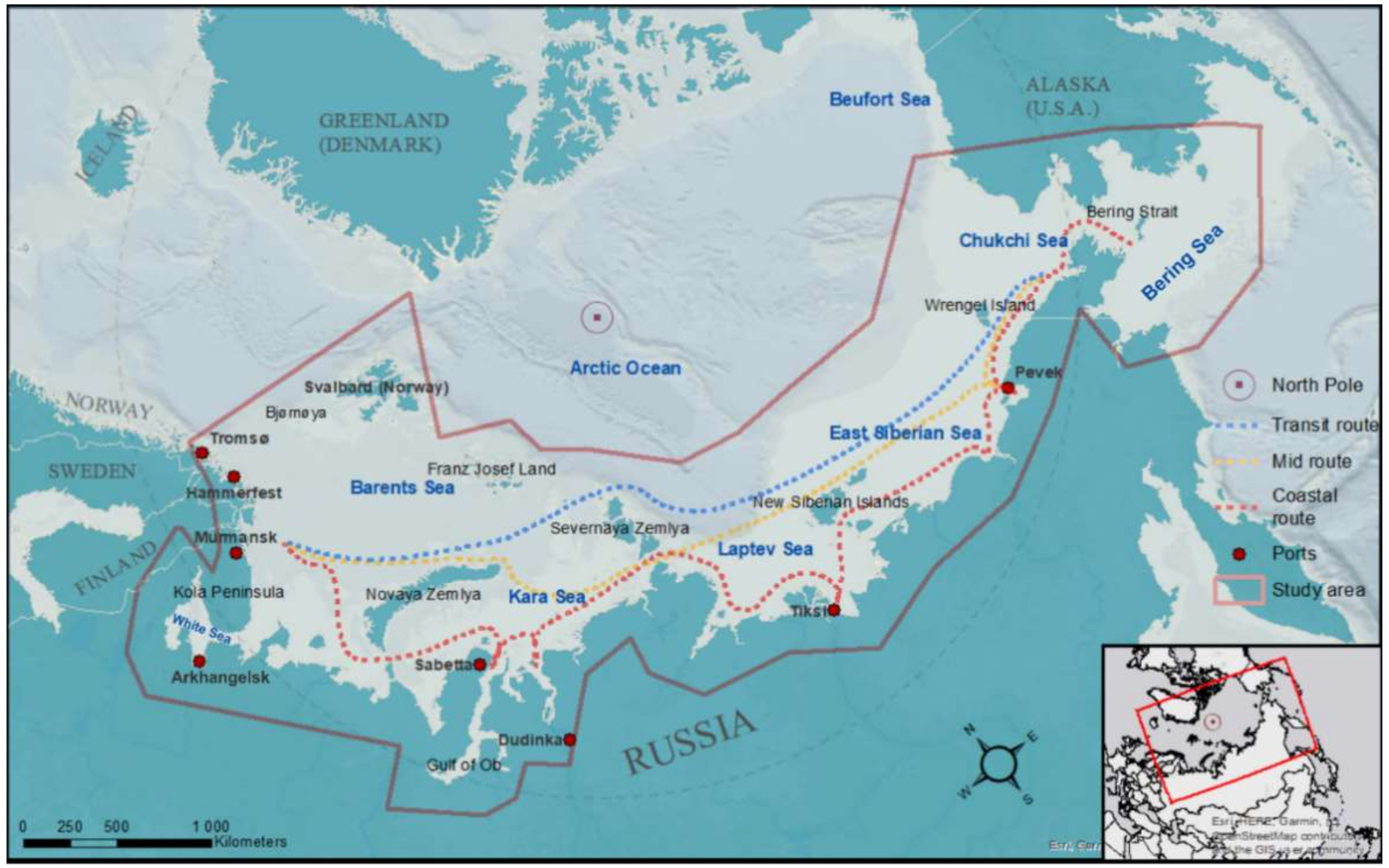
The sea route is located between 71°58′ N 26°34 E and 64°11′ N 169°05′ W and is 5000–5400 km long, stretching from the east coast of Novaya Zemlya in the west to Cape Dezhnev in the east. The NSR can be divided into three routes: (1) the Coastal Route (CR), (2) the Mid Route (MR), and (3) the Transit Route (TR) (Figure 1). The sea route is considered the shortest available connection between Northeast Asia and Northern Europe, about 2700 nautical miles shorter than the Suez Canal route [5,21]. The sea route crosses five Arctic seas: The Barents Sea, the Kara Sea, the Laptev Sea, the East Siberian Sea, and the Chukchi Sea (Figure 1). The accessibility of the sea route is heavily influenced by variable sea ice and weather conditions. Thick, first-year sea ice is the dominant ice type in the region, and ship traffic is therefore often dependent on ice breakers in the winter. However, during the summer season (July–September), the sea route can be ice-free, allowing the transit of ships without ice-breaker support [30]. The ongoing climatic change is expected to increase the accessibility and ship traffic along the sea route, which can potentially reduce travel distance by 40% and voyage time by 10 days between Asia and Northern Europe, relative to the conventional route via the Suez Canal [5,30,31,32]. According to estimations, the NSR will be economically viable by 2040 [33].
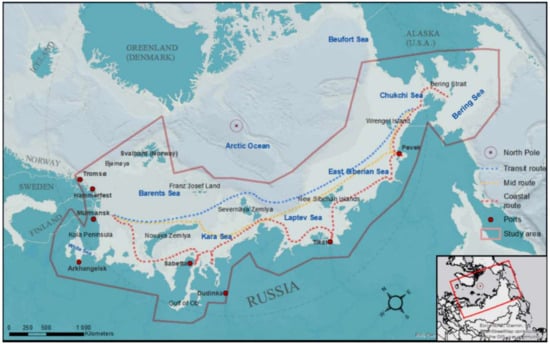
Figure 1.
Overview of the study area. Light to dark blue shading indicate ocean areas. Light color indicates shallow water, whereas dark indicates deeper water.
The NSR was commercially opened in 1935 and has, to varying degrees, been used since then [30,34]. In relation to sea ice decline and increased navigability during the 2000s, a testing phase of the feasibility of the sea route was initiated between 2010 and 2013, which rapidly increased shipping activity along the sea route. The year of 2013 was an important one, as new and more flexible rules and regulations become permanent, ultimately increasing overall ship traffic and transported cargo in the years that followed [34]. Additionally, 2013 marked the beginning of the construction of the Yamal liquefied natural gas (LNG) project, which has had a big impact on future shipping in the region. Furthermore, the number of transits peaked at 71 in 2013 but has since decreased to about 20–40 [5,21,35]. However, overall goods transportation has increased significantly, mainly due to an increase in domestic/destination shipping. From 2013 to 2019, the total annual cargo volume along the NSR increased from 1.4 to 23.5 million tonnes [35,36].
3. Materials and Methods
3.1. Data Collection
3.1.1. Ship Data
The ship traffic data of 2013 were collected from the Arctic Ship Traffic Database (ASTD) provided by the Protection of the Arctic Marine Environment (PAME). The ASTD system is based on AIS signals from ships operating in the Arctic and provides information about the ship’s type, size, position, fuel specifications, and emissions, which is generated every sixth minute and collected and stored in monthly csv-tables [37]. In this study, we collected geographical point-based ship IDs along the NSR over the year 2013. To avoid noise and erroneous signals, only ship IDs with more than 10 registrations (>1 h voyage time) were included. Number of unique ships were used as a parameter to represent the ship activity in this study. Similar parameters were also used in previous studies [18,21,34,38,39]. Ship activity analysis in this study is therefore from the viewpoints of just of number of unique ships. Other parameters such as ship speed and size were not included in the current study.
3.1.2. Emission Data
Emission data are calculated for each individual ship operating in the Arctic based on each ship’s AIS signals and their associated technical specifics (size, engine types, engine type, etc.), phases (cruising, maneuvering, hoteling, etc.), and fuel usage [37]. The calculation is performed by the ASTD system, allowing users to collect estimated emission data for CO2, NOx, SO2, PM, and BC and other gases. The emission data are calculated based on algorithms for each ship type and size and are supplemented with information from other data sources, including I ship details and information from DNV-GL. A generalized example of the methodology is as follows:
where:
denotes the emission amount of pollutant j from shIp i (g);
denotes the main engine power for sIip i (kW);
denotes the speed over ground for Ihip i at time t (knots);
denotes the maximum speed for ship i (knots);
and denote the main engine emission factor and the auxiliary engine emission factor (EF) for pollutant j, engine type k, engine tier l, and fuel type m (g/kWh), respectively;
and denote auxiliary engine power demand and the boiler power demand, respectively, in phase p for ship type i (kW);
denotes the boiler emission factor (EF) for pollutant j and fuel type m (kW).
From Equation (1), each point-based ship registration is calculated an associated emission estimation for various gases based on available ship specific information. The ship specific information used in the algorithm are not provided in the ASTD system directly. The ASTD system data can be accessed at three different levels (Levels 1, 2, or 3). Levels 2 and 3 only provide information such as ship ID (ASTD-generated), ship size, flag name, ice class, and fuel quality of each ship. Level 1, however, provides International Maritime Organization (IMO) and Maritime Mobile Service Identity (MMSI) number for each ship registration, allowing ships and their specifics to be identified [40,41]. In this study, ASTD Level 3 data were accessed.
3.2. Data Processing and Analysis
For the collected ship traffic and emission data, data points containing NaN-values, blank values, and unique ship IDs with less than 10 registrations per month (<1 h) are filtered out first, as they are considered either erroneous or noise. Then, the monthly and seasonal numbers of unique ships along the NSR in 2013 and the associated emissions of CO2, NOx, SO2, PM, and BC in 2013 were calculated in Python. The definition of seasonality in this paper is: (1) winter, including January, February, and December; (2) spring, including March, April and May; (3) summer, including June, July and August, and (4) autumn, including September, October, and November (Table 1).

Table 1.
Overview of defined seasons (months included in each season).
Each registration of a ship ID and the associated emitted amounts of CO2, NOx, SO2, PM, and BC are attached to a geographical point. In this study, the grid was created using the python library, GeoPandas (Version: 0.10.2) (https://geopandas.org/, accessed on 14 November 2021), and is made up of equally spaced 0.25 × 0.25 degrees longitude and latitude cells, using the WGS 1984 datum (https://epsg.io/4326, accessed on 14 November 2021). All point-based ship and emission data were then merged with the grid using the GeoPandas function spatial join (sjoin). This allows each grid cell to take the attributes from each data point and calculate the total number of unique ships and emissions that fall within each grid cell. Monthly and seasonal number of unique ships and associated emissions along the NSR in 2013 can then be calculated and mapped.
The grid cell area was calculated using the python libraries, Pyproj (Version: 3.3.0) (https://pypi.org/project/pyproj/, accessed on 14 November 2021) and Shapely (Version: 1.8.0) (https://pypi.org/project/Shapely/, accessed on 14 November 2021). Pyproj transformed the projected coordinate system from degrees (WGS 1984 datum) to meters, using the coordinate system WGS 84 Arctic Polar Stereographic datum (https://epsg.io/3995, accessed on 14 November 2021). Shapely calculated the area of the 0.25 × 0.25 degrees cell grids in meters, using the area function (.area).
The density of unique ship numbers and amounts of CO2, NOx, SO2, PM, and BC emissions were calculated by dividing the total number of ships or emission within each grid cell by the total area of the grid cell. For visualization purposes, the gridded data were interpolated using the python library SciPy (Version: 1.7.1) (https://docs.scipy.org/doc/scipy/, accessed on 14 November 2021) and the function griddata, using the nearest-neighbor interpolation method. The density distribution figures were created in Python, using the libraries Matplotlib (Version: 3.5.1) (https://pypi.org/project/matplotlib/, accessed on 14 November 2021) and CartoPy (Version: 0.20.2) (https://pypi.org/project/Cartopy/, accessed on 14 November 2021). The density distribution is presented in logarithmic scale for visualization purposes.
4. Results
4.1. Seasonal and Spatial Variations in Ship Traffic
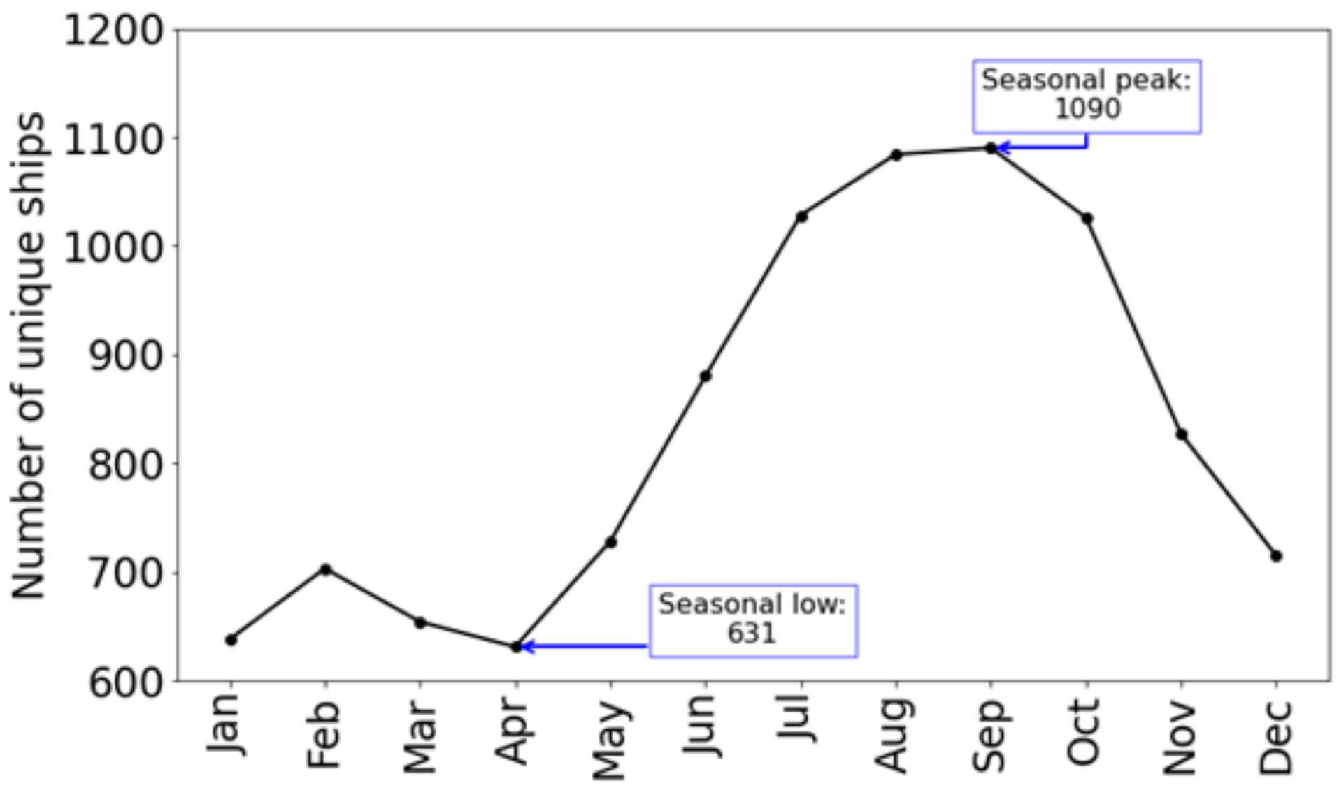
The number of unique ships along the NSR for each month in 2013 are shown in Figure 2. The unique ship numbers show a clear seasonal variation and exhibit four phases. From January to April, the number of ships was relatively low, ranging between 600 and 700 unique ships. From May to August, the number increased by 49% to 1084 unique vessels. The number remained relatively high throughout August, September, and October, with a peak of 1090 unique ships observed in September. From October to December, the number reduced significantly by 30% to 715 unique ships (Figure 2).
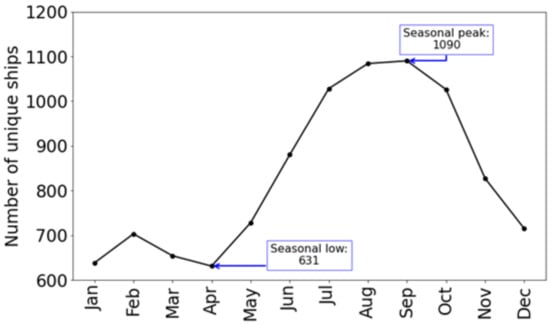
Figure 2.
Number of monthly unique ships along the NSR in 2013.
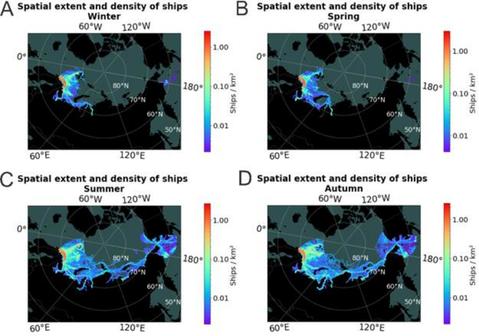
The spatial extent of total numbers in winter, spring, summer, and autumn is shown in Figure 3. The spatial extent of ship traffic in winter was relatively small. Ship traffic was mainly confined to 20–45° E and 70–77.5° N (western Barents Sea), as well as the western coast of Svalbard (Figure 3A). However, significant ship activity was observed in the Kara, White, and Bering Seas. The density of ship traffic was highest along the Norwegian coast and the western part of the Kola Peninsula, with up to 2.3 ships/km2 per grid cell. Moreover, a well-defined, shipping lane was observed in winter, stretching from the Kola Peninsula to the Gulf of Ob, hereafter referred to as the Kola–Ob lane.
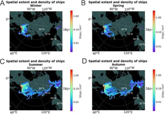
Figure 3.
Density distribution plot of total seasonal number of ships for (A) winter, (B) spring, (C) summer, and (D) autumn, along the NSR in 2013.
In spring, the spatial extent of ships was similar to that of winter (Figure 3B). However, the density of ship traffic offshore of Norway and the Kola Peninsula was slightly reduced. The northern and northeastern parts of the Barents Sea exhibited the largest reduction, with ship traffic in the south of Novaya Zemlya, along the Kola–Ob lane, exhibiting a slight reduction. In contrast, ship traffic increased along the northern shores of Novaya Zemlya, forming a northern Kola–Ob lane route. The highest density of ship traffic remained along the Norwegian coast and the Kola Peninsula, with up to 2.3 ships/km2.
Ship traffic in summer expanded both east- and northwards, covering most of the study area (Figure 3C). Areas exposed to relatively high density of ship traffic increased slightly, mainly along the Norwegian coast and the Kola Peninsula but also around Bjørnøya and Svalbard. In addition, the Kola–Ob lane expanded eastwards, forming trans-Arctic shipping lanes, which follow the transit, mid, and coastal routes of the NSR. Furthermore, an increase in ships/km2 occurred in the Bering Strait and Sea, with most of the ship traffic occurring along the coastal region of Russia and Alaska.
During autumn, the spatial extent of ship traffic was similar to that in the summer (Figure 3D). The high-density areas remained along the coastal areas of Norway and the Kola Peninsula, with up to 2.3 ships/km2. However, ship traffic in the Barents Sea (around Bjørnøya and south-southeast of Svalbard) increased in density compared to summer, exhibiting up to 0.5 ships/km2. The trans-Arctic shipping lane persisted throughout autumn, with the highest density of ships occurring along the mid-route of the NSR. Ship traffic in the Bering Strait expanded further north and eastwards into the Chukchi and Beaufort Seas.
4.2. Seasonal and Spatial Variations of Atmospheric Emissions
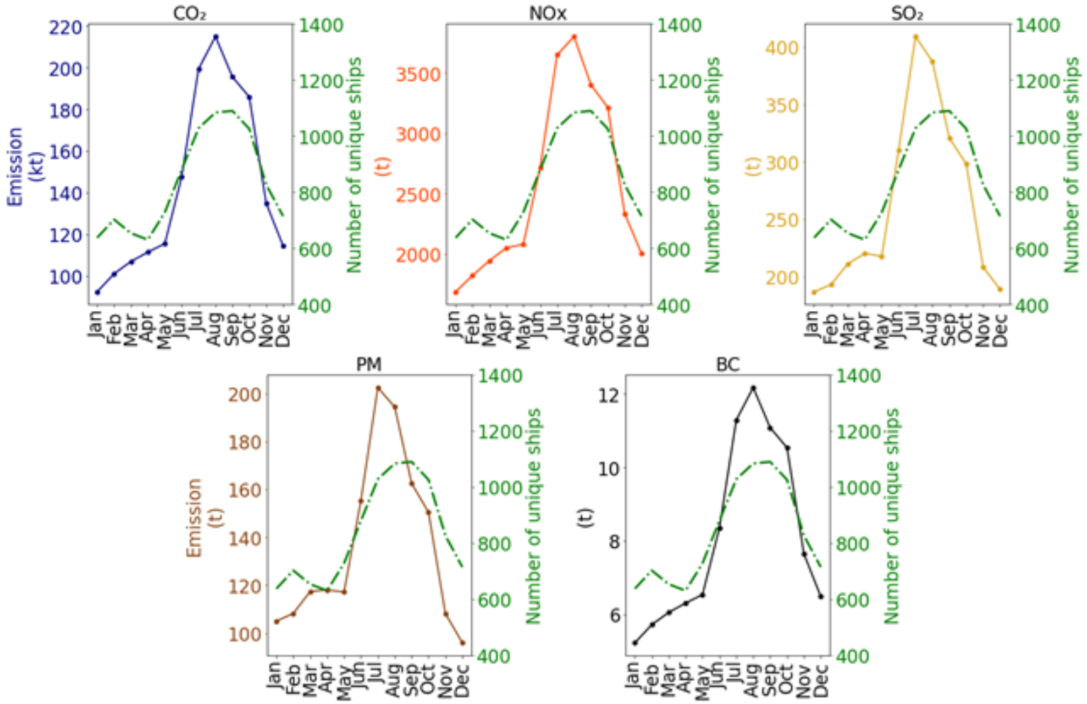
The monthly ship-associated emissions of CO2, NOx, SO2, PM, and BC are shown in Figure 4. The emissions showed obvious seasonal variations, exhibiting four phases. In winter, the emissions were relatively low, gradually increasing towards spring. The gradual increase continued in spring for CO2, NOx, and BC, whereas emissions of SO2 and PM remained at a relatively stable level. From January to May, emissions of CO2, NOx, SO2, PM, and BC gradually increased by 25%, 23%, 17%, 12%, and 25%, respectively. In summer, emissions of CO2, NOx, SO2, PM, and BC almost doubled, increasing by 86%, 83%, 88%, 73%, and 86%, respectively. For CO2, NOx, and BC, the peaks were observed in August, whereas SO2 and PM peaked in July. After the observed peaks in summer, the atmospheric emissions gradually decreased during autumn but remained at a relatively high level. By October, emissions of CO2, NOx, SO2, PM, and BC decreased by 13%, 15%, 27%, 26%, and 13%, respectively. A sharp decrease in emissions was observed from October to November, with emissions of CO2, NOx, SO2, PM, and BC reducing by 27%, 27%, 30%, 28%, and 27%, respectively.
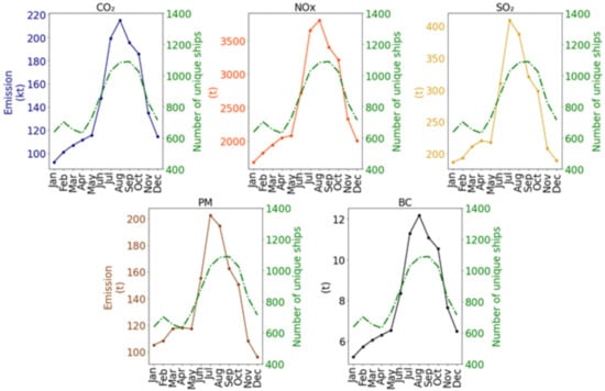
Figure 4.
Monthly emission of the atmospheric pollutants CO2, NOx, SO2, PM, and BC and number of unique ships along the NSR for the year 2013. Note that CO2 emissions are given in kilotons (kt).
In general, emissions showed large seasonal variability, with summer and autumn accounting for 62.7% (32.7% and 30.0%, respectively) of the annual emission inventory, whereas winter and spring accounted for 37.3% (17.9% and 19.4%, respectively).
The spatial emission densities of CO2 and SO2 in winter, spring, summer, and autumn are shown in Figure 5 and Figure 6 (the emission densities of CO2 are similar to that of NOx and BC, whereas the emission density of SO2 is similar to that of PM. More details on the spatial emission densities for NOx, PM, and BC are provided in Supplementary Figures S1–S3).
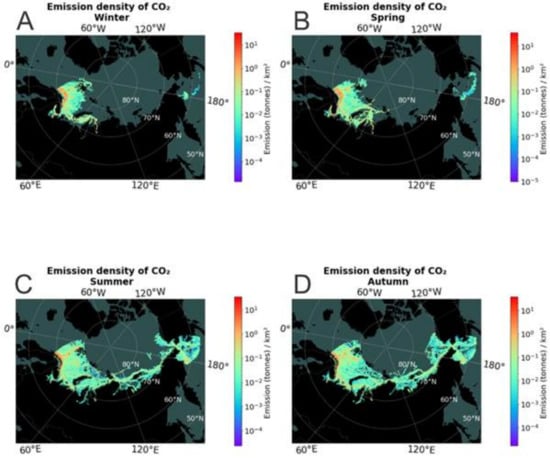
Figure 5.
Density distribution of CO2 emissions for the seasons (A) winter, (B) spring, (C) summer, and (D) autumn along the NSR in 2013.
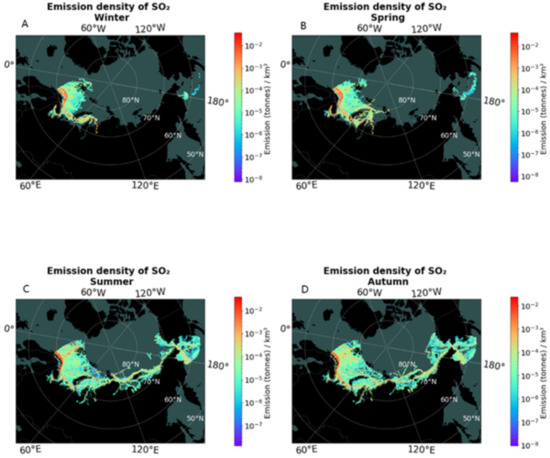
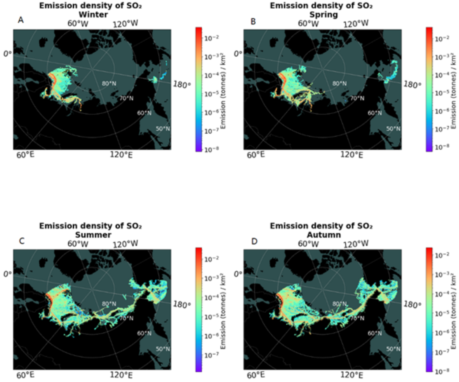
Figure 6.
Density distribution of SO2 emissions for the seasons (A) winter, (B) spring, (C) summer, and (D) autumn along the NSR in 2013.
In winter, the spatial distribution of atmospheric emissions was confined to a small area, between 20–45° E and 70–77.5° N (western Barents Sea) (Figure 5A and Figure 6A). The highest emissions were observed along the coastal areas of Norway, the Kola Peninsula, and the Kola–Ob lane and between Svalbard and Bjørnøya. Additionally, emissions of a small spatial extent were also observed in the Bering Sea (Figure 5A and Figure 6A). The emissions of CO2, NOx, SO2 PM, and BC in areas of high exposure to emissions were up to 32, 0.50, 0.037, 0.017, and 0.0019 t/km2, respectively. The emission densities of CO2, NOx, and BC decreased towards the east (Figure 5A), along the Kola–Ob lane, whereas the emission density of SO2 and PM remained high along the Kola–Ob lane (Figure 6A). In the Barents Sea, densities of all emissions were similar.
In spring, the spatial extent of emissions extended north- and eastwards, now covering the majority of the Barents Sea. In addition, a large portion of the Kara Sea was exposed to ship-associated emissions (Figure 5B and Figure 6B). Furthermore, the Kola–Ob lane was split into two lanes, the coastal Kola–Ob lane and the northern Kola–Ob lane. Emission density along the coastal lane reduced while increasing along the newly formed northern Kola–Ob lane, north of Novaya Zemlya. In the Bering Sea, emissions’ spatial extent increased, whereas their density decreased. In spring, the emissions of CO2, NOx, SO2, PM, and BC in areas of high exposure to emissions reached 39, 0.59, 0.042, 0.020, and 0.0022 t/km2, respectively. The emission densities of SO2 and PM remained relatively high along the shipping lanes stretching east of the Norwegian and Kola coastal areas, whereas the densities of CO2, NOx, and BC emissions decreased eastwards but remained relatively high in the Gulf of Ob.
In summer, the spatial distribution of emissions further extended to cover the entire study area, forming the trans-Arctic shipping lanes (Figure 5C and Figure 6C). The entire Barents and Kara Seas, and the coastal areas of Laptev, East Siberian, Chukchi, and Bering Seas were, to varying degrees, exposed to ship-associated emissions. Areas along the western coast of Svalbard and the Bering Strait and Sea were now exposed to increased emissions, with the highest/largest increase observed in the Bering Strait and Sea. In summer, emissions of CO2, NOx, SO2, PM, and BC in high emission exposure areas increased, reaching densities of up to 54.66, 0.85, 0.059, 0.028, and 0.0031 t/km2, respectively. Differences between the emission densities of CO2, NOx, and BC and those of SO2 and PM were, in general, less clear. Only slightly higher emissions of SO2 and PM were observed along the Kola–Ob lane, the trans-Arctic lanes, and between Norway and Svalbard.
In autumn, the spatial extent of emissions remained high and increased in the Chukchi Sea. The highest emissions remained along the coast of Norway and the Kola Peninsula and eastwards towards the Gulf of Ob (Figure 5D and Figure 6D). Emissions in the Barents Sea and along the southern coast of Svalbard increased relative to summer. At 60° E and eastwards, the emissions were similar to those in the summer. However, emissions in the trans-Arctic shipping lanes were slightly denser in autumn than in summer, especially along the coastal route. In autumn, emissions of CO2, NOx, SO2, PM, and BC in high emission exposure areas decreased, exhibiting densities of up to 46.29, 0.72, 0.050, 0.022, and 0.0026 t/km2, respectively. Emission densities of CO2, NOx BC, SO2, and PM remained relatively high along the coastal route of the NSR (Figure 5D and Figure 6D). In contrast to CO2, SO2 displayed high emission densities along the mid-route (Figure 6D).
5. Discussion
5.1. Seasonal and Spatial Variation in Ship Traffic
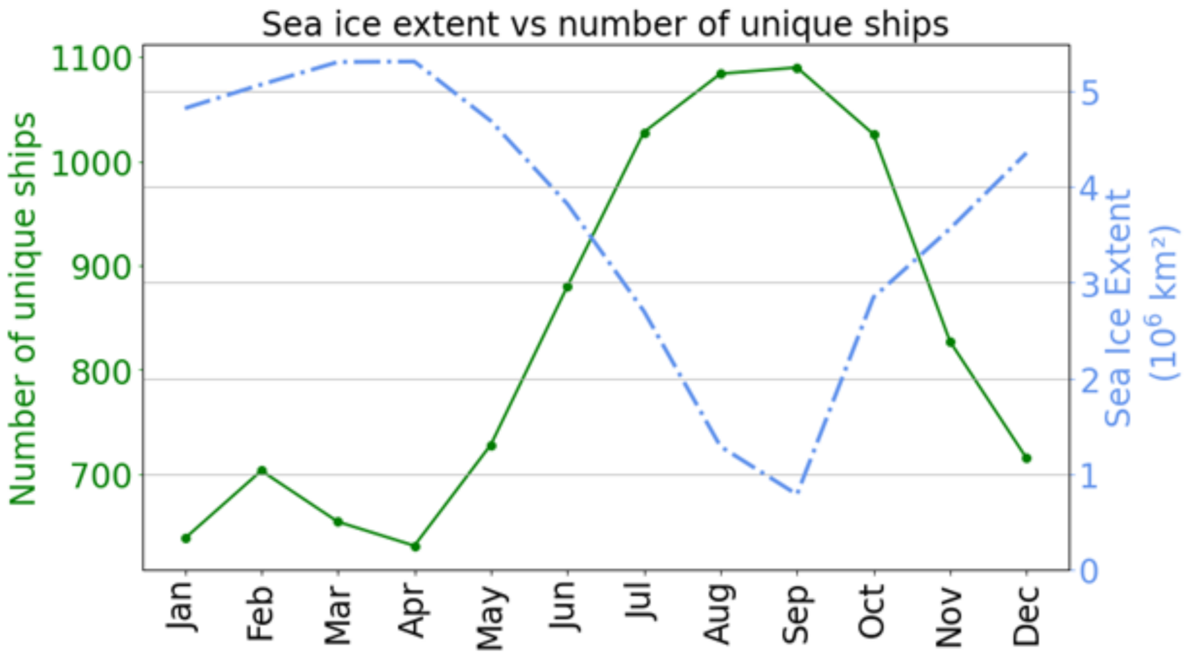
The results showed large seasonal variability in ship traffic. The number of unique ships is relatively low in winter and spring, and considerably higher in summer and autumn (Figure 2 and Figure 3). Other studies showed similar seasonal trends, with the highest ship traffic (number of vessels, voyages, or amount of distance traveled) occurring between July and October, especially along the NSR and >70° N [4,20,21,39]. The seasonality in Arctic shipping is often linked to the presence of sea ice, as it is considered a key constraint for accessibility of non-ice strengthened vessels [4,20,32]. Figure 7 shows the number of unique ships and sea ice extent in the study area in 2013. Sea ice extent has an inverse relationship with number of unique ships. From April to September, the extent of sea ice decreased by 85%, whereas number of ships increased by 75% (Figure 7).
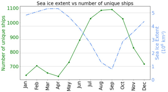
Figure 7.
Monthly sea ice extent and number of unique ships in the study area in 2013. Sea ice data provided from NSIDC [42]. For exact numbers and sea ice coverage of the marine area, see Table S1 in Supplementary Files).
The spatial distribution of ships’ activity exhibits large seasonal variation. In winter and spring, ship traffic was confined to the Norwegian and Barents Seas (Figure 3A,B). Throughout summer and autumn, ship traffic expanded to most of the study area, forming the clear trans-Arctic shipping lane and the Kola–Ob shipping lane (Figure 3C,D).
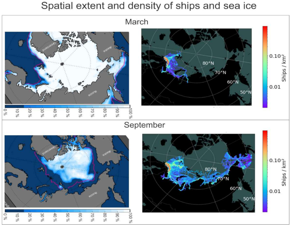
Similar to temporal variations in number of unique ships, the seasonal spatial distribution of ships displays an inverse relationship with the regional sea ice conditions. Figure 8 shows a comparison between sea ice concentration [42] and the spatial distribution of ship densities in March and September 2013. In March, the NSR was covered by sea ice (90–100% concentration), and ship traffic was absent east of the Gulf of Ob. In September, sea ice was absent along the majority of the NSR, excepting a small patch in the strait between Severnaya Zemlya and the Russian mainland (20–70% concentration), and ship traffic was present.
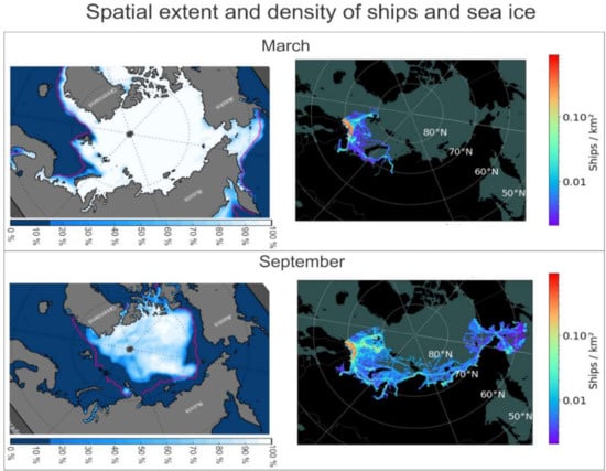
Figure 8.
Spatial extent and density of ships and concentration of sea ice along the NSR in March and September 2013. Sea ice concentration maps by courtesy of the National Snow and Ice Data Center (NSIDC), University of Colorado, Boulder (www.nsidc.org, accessed 23 November 2021).
However, sea ice is not the only factor determining ship traffic in this region [43,44]. The year-round Kola–Ob shipping lane transits areas covered by seasonally dense sea ice, due to multiple ice-strengthened vessels transporting metals and gas condensate from Dudinka to Murmansk or Europe [21]. This highlights the potential that factors other than sea ice have for the development of ship activity in the area, such as global economy, regional infrastructure (i.e., access to ice-strengthened ships), and regulations (i.e., IMO Polar Code and transit fees) [21,34,43,44,45].
5.2. Seasonal Variations in Ship-Associated Emissions
Similarly to ship traffic, emissions of CO2, NOx, SO2, PM, and BC exhibit large seasonal variations. In winter and spring, emissions are relatively low, whereas they increase significantly during summer and remain high throughout autumn. Similar findings have been observed in other studies concerning the Arctic as a whole [12,15,23,24]. The increase in emissions is linked with the overall increase in ship traffic during summer and autumn (and the associated fuel consumption) [24,46].
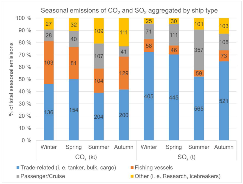
In addition, ship type is also an important factor for the seasonality in emissions. On comparing the seasonal emissions of CO2 and SO2 by ship type, the emission contributions from different ship types in summer and autumn differ from those in winter and spring (Figure 9). For CO2, the contribution from passenger/cruise ships and other ship types (i.e., research and icebreakers) doubles from spring and winter to summer (about ~20% to over 40% combined contribution), suggesting that the overall increase in emissions is heavily influenced by the increased activity of certain ship types. This is also evident for SO2, where the contribution from passenger/cruise ships exhibits the largest change, accounting for more than 30% of the total emissions in summer but contributing only 10–15% of the total emissions in winter, spring and autumn. The sudden increase in SO2 emissions from passenger/cruise ships is likely to be related to the July peak observed for SO2 and PM emissions. Cruise ships are generally energy-demanding and active during July [40,47,48].
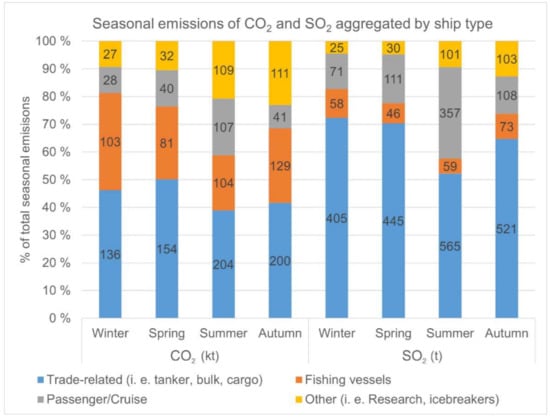
Figure 9.
Seasonal contribution of CO2 and SO2 emissions aggregated by ship type. The contribution by ship type in% is given in the y-axis, whereas the contribution in kt (CO2) and t (SO2) is given inside the bars.
Furthermore, the increase in SO2 emissions suggests an increased usage of heavy fuel oil (HFO), as HFO has a higher sulfur content, resulting in higher SO2 and PM emissions [11,25,26], with cruise ships accounting for a large portion of the Arctic HFO usage [49,50]. Based on other studies, the sudden increase in SO2 also implies an increase in larger, trade-related ship types (i.e., tankers and bulk and cargo vessels) [10,50].
The spatial distribution of shipping-associated emissions exhibits large seasonal variability, which is similar to the variations observed in ship traffic. The highest emissions occur in areas with the highest density of ship traffic, particularly for CO2, Nox, and BC (i.e., the coastal area of Norway and the Kola Peninsula) and decrease accordingly in areas with less ship traffic, as suggested in other studies [24,28]. Additionally, there are areas with relatively low densities of ships that exhibit relatively high emissions of SO2 and PM when compared to high-density areas (i.e., the Kola–Ob and the trans-Arctic shipping lanes (60–180° E)) (Figure 8). This suggests a relatively high HFO usage, which, according to studies conducted by the International Council on Clean Transportation, is considerably higher in Russian than in Norwegian waters [49].
5.3. Implications for the Future
From the above results, this study suggests that, given a permanent melt in sea ice along the sea route, as other studies suggest [51,52,53], the potential for trade-related shipping activities increases. Alongside trade-related shipping, the overall emissions will increase significantly, covering larger areas, with spatial and temporal similarities to the summer/autumn emission scenario of 2013. Furthermore, this will increase the formation of secondary pollutants, such as tropospheric ozone, nitrate, sulfate, and ammonium aerosols and hydroxyl radicals (OH), as other studies have previously shown, and cause negative impacts on the Arctic environment [18,24,26,28]. Studies on the seasonal and spatial variability in the following years (2014–2021) and a comparison of the variabilities within the years are suggested in the future. Furthermore, an investigation on the impact of these seasonal variations on the environment is needed for better adaptation and sustainable development of future Arctic operations.
6. Conclusions
In this study, we investigated the seasonal and spatial distribution of shipping activity and the associated atmospheric emissions along the NSR and surrounding areas in 2013. The results showed that ship traffic showed significant seasonal and spatial variations. In winter and spring, ship traffic was generally low and limited to the Barents Sea, whereas the number of ships increased and expanded rapidly eastwards throughout summer, covering most of the study area and forming trans-Arctic shipping lanes. Ship traffic activity remained high throughout autumn, exhibiting slightly denser traffic in the Barents Sea and along the mid-route of the NSR. In general, emissions reflect the temporal and spatial variations observed for ship traffic, especially for CO2, NOx, and BC, whose densities are low during winter and spring and high during summer and autumn. The monthly emission peaks of SO2 and PM are observed one month prior to those for CO2, NOx, and BC. This might be linked to the changes in ship types, which diversify during summer and autumn, especially for cruise/passenger ships during summer. The spatial distribution of the emissions extends eastwards in summer and remains high throughout autumn. Most emissions occur along the high-traffic coastal areas of Norway and the Kola-Peninsula, the Barents Sea, and Svalbard, but decrease further east. The emissions of SO2 and PM were relatively high when compared to the observed number of ships along the various shipping lanes (Kola–Ob and trans-Arctic). The results from this study are of great importance for people working in Arctic maritime-related sectors such as shipping industries and for Arctic communities, decision-makers, and researchers.
Supplementary Materials
The following are available online at https://www.mdpi.com/article/10.3390/su14031359/s1, Figure S1: Density distribution of NOx emissions for the seasons (a) winter, (b) spring, (c) summer and (d) autumn along the NSR in 2013., Figure S2: Density distribution of PM emissions for the seasons (a) winter, (b) spring, (c) summer and (d) autumn along the NSR in 2013., Figure S3: Density distribution of BC emissions for the seasons (a) winter, (b) spring, (c) summer and (d) autumn along the NSR in 2013. Table S1: Monthly sea ice extent, sea ice coverage (% of study areas marine area) and number of unique ships in the study area in 2013.
Author Contributions
N.F.: writing—original draft, conceptualization, methodology, formal analysis, investigation, and visualization; J.L.: writing—review and editing, conceptualization, supervision, and project administration. All authors have read and agreed to the published version of the manuscript.
Funding
This research received no external funding.
Institutional Review Board Statement
Not applicable.
Informed Consent Statement
Not applicable.
Data Availability Statement
The data presented in this study are available on request from the corresponding author.
Acknowledgments
The authors would like to acknowledge the Department of Technology and Safety, UiT—The Arctic University of Norway, for their support to this research. Thanks Tuomas Heiskanen for his valuable help in data analysis and Python-debugging.
Conflicts of Interest
The authors declare that they have no known competing financial interest or personal relationships that could have appeared to influence the work reported in this paper.
References
- Yumashev, D.; van Hussen, K.; Gille, J.; Whiteman, G. Towards a Balanced View of Arctic Shipping: Estimating Economic Impacts of Emissions from Increased Traffic on the Northern Sea Route. Clim. Change 2017, 143, 143–155. [Google Scholar] [CrossRef] [Green Version]
- Dawson, J.; Carter, N.; van Luijk, N.; Parker, C.; Weber, M.; Cook, A.; Grey, K.; Provencher, J. Infusing Inuit and Local Knowledge into the Low Impact Shipping Corridors: An Adaptation to Increased Shipping Activity and Climate Change in Arctic Canada. Environ. Sci. Policy 2020, 105, 19–36. [Google Scholar] [CrossRef]
- PAME. The Increase in Arctic Shipping—Arctic Shipping Status Report #1; PAME: Akureyri, Iceland, 2020. [Google Scholar]
- Berkman, P.A.; Fiske, G.; Røyset, J.-A.; Brigham, L.W.; Lorenzini, D. Next-Generation Arctic Marine Shipping Assessments. In Governing Arctic Seas: Regional Lessons from the Bering Strait and Barents Sea, 1st ed.; Young, O., Berkman, P., Vylegzhanin, A., Eds.; Springer Nature: Cham, Switzerland, 2018. [Google Scholar] [CrossRef]
- Aksenov, Y.; Popova, E.E.; Yool, A.; Nurser, A.J.G.; Williams, T.D.; Bertino, L.; Bergh, J. On the Future Navigability of Arctic Sea Routes: High-Resolution Projections of the Arctic Ocean and Sea Ice. Mar. Policy 2017, 75, 300–317. [Google Scholar] [CrossRef] [Green Version]
- Khon, V.C.; Mokhov, I.I.; Semenov, V.A. Transit Navigation through Northern Sea Route from Satellite Data and CMIP5 Simulations. Environ. Res. Lett. 2017, 12, 024010. [Google Scholar] [CrossRef] [Green Version]
- Melia, N.; Haines, K.; Hawkins, E.; Day, J.J. Towards Seasonal Arctic Shipping Route Predictions. Environ. Res. Lett. 2017, 12, 084005. [Google Scholar] [CrossRef]
- Stephenson, S.R.; Wang, W.; Zender, C.S.; Wang, H.; Davis, S.J.; Rasch, P.J. Climatic Responses to Future Trans-Arctic Shipping. Geophys. Res. Lett. 2018, 45, 9898–9908. [Google Scholar] [CrossRef]
- DNV. HFO in the Arctic—Phase 2; Klima-og Forurensningsdirektoratet: Oslo, Norway, 2013. [Google Scholar]
- DNV GL. Alternative Fuels in the Arctic; PAME: Haugesund, Norway, 2019. [Google Scholar]
- IMO. Fourth IMO GHG Study; IMO: London, UK, 2020. [Google Scholar]
- Corbett, J.J.; Lack, D.A.; Winebrake, J.J.; Harder, S.; Silberman, J.A.; Gold, M. Arctic Shipping Emissions Inventories and Future Scenarios. Atmos. Chem. Phys. 2010, 10, 9689–9704. [Google Scholar] [CrossRef] [Green Version]
- European Environment Agency. The Impact of International Shipping on European Air Quality and Climate Forcing; European Environment Agency: Copenhagen, Denmark, 2013. [Google Scholar] [CrossRef]
- Eyring, V.; Isaksen, I.S.A.; Berntsen, T.; Collins, W.J.; Corbett, J.J.; Endresen, O.; Grainger, R.G.; Moldanova, J.; Schlager, H.; Stevenson, D.S. Transport Impacts on Atmosphere and Climate: Shipping. Atmos. Environ. 2010, 44, 4735–4771. [Google Scholar] [CrossRef]
- Marelle, L.; Thomas, J.L.; Raut, J.C.; Law, K.S.; Jalkanen, J.P.; Johansson, L.; Roiger, A.; Schlager, H.; Kim, J.; Reiter, A.; et al. Air Quality and Radiative Impacts of Arctic Shipping Emissions in the Summertime in Northern Norway: From the Local to the Regional Scale. Atmos. Chem. Phys. 2016, 4, 2359–2379. [Google Scholar] [CrossRef] [Green Version]
- Schröder, C.; Reimer, N.; Jochmann, P. Environmental Impact of Exhaust Emissions by Arctic Shipping. Ambio 2017, 46, 400–409. [Google Scholar] [CrossRef] [Green Version]
- Sharafian, A.; Blomerus, P.; Mérida, W. Natural Gas as a Ship Fuel: Assessment of Greenhouse Gas and Air Pollutant Reduction Potential. Energy Policy 2019, 131, 332–346. [Google Scholar] [CrossRef]
- Eckhardt, S.; Hermansen, O.; Grythe, H.; Fiebig, M.; Stebel, K.; Cassiani, M.; Baecklund, A.; Stohl, A. The Influence of Cruise Ship Emissions on Air Pollution in Svalbard—A Harbinger of a More Polluted Arctic? Atmos. Chem. Phys. 2013, 13, 8401–8409. [Google Scholar] [CrossRef] [Green Version]
- Schmale, J.; Arnold, S.R.; Law, K.S.; Thorp, T.; Anenberg, S.; Simpson, W.R.; Mao, J.; Pratt, K.A. Local Arctic Air Pollution: A Neglected but Serious Problem. Earth Future 2018, 6, 1385–1412. [Google Scholar] [CrossRef]
- Eguíluz, V.M.; Fernández-Gracia, J.; Irigoien, X.; Duarte, C.M. A Quantitative Assessment of Arctic Shipping in 2010–2014. Sci. Rep. 2016, 6, 30682. [Google Scholar] [CrossRef] [PubMed] [Green Version]
- Gunnarsson, B. Recent Ship Traffic and Developing Shipping Trends on the Northern Sea Route—Policy Implications for Future Arctic Shipping. Mar. Policy 2021, 124, 104369. [Google Scholar] [CrossRef]
- Bencs, L.; Horemans, B.; Buczyńska, A.J.; Deutsch, F.; Degraeuwe, B.; Van Poppel, M.; Van Grieken, R. Seasonality of Ship Emission Related Atmospheric Pollution over Coastal and Open Waters of the North Sea. Atmos. Environ. X 2020, 7, 100077. [Google Scholar] [CrossRef]
- Winther, M.; Christensen, J.H.; Plejdrup, M.S.; Ravn, E.S.; Eriksson, Ó.F.; Kristensen, H.O. Emission Inventories for Ships in the Arctic Based on Satellite Sampled AIS Data. Atmos. Environ. 2014, 91, 1–14. [Google Scholar] [CrossRef]
- Winther, M.; Christensen, J.H.; Angelidis, I.; Ravn, E.S. Emissions from Shipping in the Arctic from 2012–2016 and Emissions Projections for 2020, 2030 and 2050; Aarhus University; DCE—Danish Centre for Environment and Energy: Aarhus, Denmark, 2017. [Google Scholar]
- Jalkanen, J.P.; Johansson, L.; Kukkonen, J.; Brink, A.; Kalli, J.; Stipa, T. Extension of an Assessment Model of Ship Traffic Exhaust Emissions for Particulate Matter and Carbon Monoxide. Atmos. Chem. Phys. 2012, 12, 2641–2659. [Google Scholar] [CrossRef] [Green Version]
- Dalsøren, S.B.; Eide, M.S.; Endresen, O.; Mjelde, A.; Gravir, G.; Isaksen, I.S.A. Update on Emissions and Environmental Impacts from the International Fleet of Ships: The Contribution from Major Ship Types and Ports. Atmos. Chem. Phys. 2009, 9, 2171–2194. [Google Scholar] [CrossRef] [Green Version]
- Ødemark, K.; Dalsøren, S.B.; Samset, B.H.; Berntsen, T.K.; Fuglestvedt, J.S.; Myhre, G. Short-Lived Climate Forcers from Current Shipping and Petroleum Activities in the Arctic. Atmos. Chem. Phys. 2012, 12, 1979–1993. [Google Scholar] [CrossRef] [Green Version]
- Marelle, L.; Raut, J.C.; Law, K.S.; Duclaux, O. Current and Future Arctic Aerosols and Ozone from Remote Emissions and Emerging Local Sources—Modeled Source Contributions and Radiative Effects. J. Geophys. Res. Atmos. 2018, 123, 12942–12963. [Google Scholar] [CrossRef]
- Moe, A.; Schram Stokke, O. Asian Countries and Arctic Shipping: Policies, Interests and Footprints on Governance. Arct. Rev. Law Polit. 2019, 10, 24–52. [Google Scholar] [CrossRef] [Green Version]
- Liu, M.; Kronbak, J. The Potential Economic Viability of Using the Northern Sea Route (NSR) as an Alternative Route between Asia and Europe. J. Transp. Geogr. 2010, 18, 434–444. [Google Scholar] [CrossRef]
- Lindstad, H.; Bright, R.M.; Strømman, A.H. Economic Savings Linked to Future Arctic Shipping Trade Are at Odds with Climate Change Mitigation. Transp. Policy 2016, 45, 24–30. [Google Scholar] [CrossRef] [Green Version]
- Stephenson, S.R.; Brigham, L.W.; Smith, L.C. Marine Accessibility along Russia’s Northern Sea Route. Polar Geogr. 2014, 37, 111–133. [Google Scholar] [CrossRef]
- Ørts Hansen, C.; Grønsedt, P.; Lindstrøm Graversen, C.; Hendriksen, C. Arctic Shipping—Commercial Opportunities and Challenges; CBS Maritime: Frederiksberg, Denmark, 2016. [Google Scholar]
- Gunnarsson, B.; Moe, A. Ten Years of International Shipping on the Northern Sea Route: Trends and Challenges. Arct. Rev. Law Polit. 2021, 12, 4–30. [Google Scholar] [CrossRef]
- Humpert, M. Arctic Shipping: An Analysis of the 2013 Northern Sea Route Season; The Arctic Insitute: Washington, DC, USA, 2014. [Google Scholar]
- The Northern Sea Route Information Office. About 23 Million Tons Transported along NSR in 9 Months of 2020. Available online: https://arctic-lio.com/about-23-million-tons-transported-along-nsr-in-9-months-of-2020/ (accessed on 8 October 2021).
- PAME. ASTD Data Document. Available online: https://pame.is/images/03_Projects/ASTD/Documents/ASTD_data/ASTD_Data_20_March.pdf (accessed on 14 November 2021).
- Silber, G.K.; Adams, J.D. Vessel Operations in the Arctic, 2015–2017. Front. Mar. Sci. 2019, 6, 573. [Google Scholar] [CrossRef]
- Stocker, A.N.; Renner, A.H.H.; Knol-Kauffman, M. Sea Ice Variability and Maritime Activity around Svalbard in the Period 2012–2019. Sci. Rep. 2020, 10, 17043. [Google Scholar] [CrossRef]
- PAME. Access to the Arctic Ship Traffic Data System. Available online: https://pame.is/images/03_Projects/ASTD/Documents/ASTD_Access/Access_to_ASTD.pdf (accessed on 14 November 2021).
- PAME. ASTD Data Document. Available online: https://pame.is/images/03_Projects/ASTD/Documents/ASTD_data/ASTD_Data_v1.4_June_2021.pdf (accessed on 14 November 2021).
- Fetterer, F.; Knowles, K.; Meier, W.N.; Savoie, M.; Windnagel, A.K. Sea Ice Index, version 3: Sea ice extent; NSIDC: Boulder, CO, USA. Available online: https://nsidc.org/data/G02135/versions/3 (accessed on 23 November 2021).
- Stephenson, S.R.; Smith, L.C.; Brigham, L.W.; Agnew, J.A. Projected 21st-Century Changes to Arctic Marine Access. Clim. Change 2013, 118, 885–899. [Google Scholar] [CrossRef] [Green Version]
- Stephenson, S.R.; Smith, L.C. Influence of Climate Model Variability on Projected Arctic Shipping Futures. Earth Future 2015, 3, 331–343. [Google Scholar] [CrossRef] [Green Version]
- Bennett, M.M.; Stephenson, S.R.; Yang, K.; Bravo, M.T.; De Jonghe, B. The Opening of the Transpolar Sea Route: Logistical, Geopolitical, Environmental, and Socioeconomic Impacts. Mar. Policy 2020, 121, 104178. [Google Scholar] [CrossRef]
- Olmer, N.; Comer, B.; Roy, B.; Mao, X.; Rutherford, D. Greenhouse Gas Emissions From Global Shipping, 2013–2015; The International Council on Clean Transportation: Washington, DC, USA, 2017. [Google Scholar]
- Simonsen, M.; Walnum, H.J.; Gössling, S. Model for Estimation of Fuel Consumption of Cruise Ships. Energies 2018, 11, 1059. [Google Scholar] [CrossRef] [Green Version]
- Simonsen, M. Cruise Ship Tourism—A LCA Analysis; Western Norway Research Institution: Sogndal, Norway, 2014. [Google Scholar]
- Comer, B.; Osipova, L.; Georgeff, E.; Mao, X. The International Maritime Organization’s Proposed Arctic Heavy Fuel Oil Ban: Likely Implications and Opportunities for Improvement; The International Council on Clean Transportation: Washington, DC, USA, 2020. [Google Scholar]
- Comer, B.; Olmer, N.; Mao, X.; Roy, B.; Rutherford, D. Prevalence of Heavy Fuel Oil and Black Carbon in Arctic Shipping, 2015 to 2025; The International Council on Clean Transportation: Washington, DC, USA, 2017. [Google Scholar]
- Cohen, J.; Zhang, X.; Francis, J.; Jung, T.; Kwok, R.; Overland, J.; Ballinger, T.J.; Bhatt, U.S.; Chen, H.W.; Coumou, D.; et al. Divergent Consensuses on Arctic Amplification Influence on Midlatitude Severe Winter Weather. Nat. Clim. Chang. 2020, 10, 20–29. [Google Scholar] [CrossRef]
- SIMIP, C. Arctic Sea Ice in CMIP6. Geophys. Res. Lett. 2020, 47, e2019GL086749. [Google Scholar] [CrossRef]
- Smith, D.M.; Screen, J.A.; Deser, C.; Cohen, J.; Fyfe, J.C.; García-Serrano, J.; Jung, T.; Kattsov, V.; Matei, D.; Msadek, R.; et al. The Polar Amplification Model Intercomparison Project (PAMIP) Contribution to CMIP6: Investigating the Causes and Consequences of Polar Amplification. Geosci. Model Dev. 2019, 12, 1139–1164. [Google Scholar] [CrossRef] [Green Version]

Publisher’s Note: MDPI stays neutral with regard to jurisdictional claims in published maps and institutional affiliations. |
© 2022 by the authors. Licensee MDPI, Basel, Switzerland. This article is an open access article distributed under the terms and conditions of the Creative Commons Attribution (CC BY) license (https://creativecommons.org/licenses/by/4.0/).