Analyzing Tehran’s Air Pollution Using System Dynamics Approach

Abstract

Air pollution is one of the major issues in urban management. City managers and planners pay a great deal of attention to this problem given its harmful effect on people’s health and the environment. This paper proposes a simulated model of the pollution level of the capital city of Tehran along with its source and outcomes based on system dynamics. First, it provides a comprehensive review of the sources of greenhouse emission along with the impact of natural factors on its growth. The data is collected from 2011 to 2021. Then a dynamic model is applied to simulate Tehran’s air pollution for twenty years (from 2011 to 2031). The statistical method of design of experiments (DoE) is considered to set the sensitive and controllable variables of the city’s pollution. The information is used to set plans to reduce the air pollution considering several scenarios. The results of the research show that the best strategy to reduce air pollution that can resolve other issues as well is to manufacture environmentally friendly cars that can rely on renewable energy resources as their fuels. The other highly important strategy is to preserve forests.

1. Introduction

Air is vital for the maintenance of human life and also necessary for other creatures on planet Earth. Without air, no one could ever keep on living for more than a few minutes. Air is made up of gases such as nitrogen, oxygen, carbon dioxide, and other gases [1,2]. A slight change in its composition may result in unpleasant atmospheric conditions for humans and the environment around them. This is called air pollution. Air pollution is a serious environmental issue, particularly in developing countries.

The path of air pollution in the city involves emission and expansion of air pollutants resulting from various factors. Throughout the path, air pollutants are dispersed via various dispersion pathways (air, water, soil, living organisms) thinning and undergoing chemical reactions [3]. In other words, the phenomenon of air pollution is a series including various events such as generation and dispersion of the pollutants from their source, their conversion, transmission, and emission into the atmosphere, and their impact on humans, materials, and the ecosystem [4]. Additionally, air pollution is a major health issue in developing countries. Despite better air quality in the last 50 years, air pollution still reduces the life span of humans and causes a large number of people to go to hospitals. It also causes much harm to the natural environment such that frequent studies indicate that people notice air pollution constantly, especially in urban and industrial regions. Furthermore, epidemiological studies in the last two decades have shown that air pollution is one of the leading causes of death [5]. On the other hand, industrialization and population growth play the main role in air pollution. Air pollution is attributed to an increase in the concentration of greenhouse gases (air pollutants). Air pollutants are classified into several categories.

1.1. Primary and Secondary Pollutants

Primary pollutants enter the atmosphere directly from the source and include: (1) carbon compounds, such as CO, CO₂, CH₄, and VOCs; (2) nitrogen compounds, such as NO, N₂O, and NH₃; (3) sulfur compounds, such as H₂S and SO₂; (4) halogenated compounds, such as chloride, fluoride, and bromide; and (5) particulate matter (PM) or “aerosols”.

Secondary pollutants are those which do not get into the atmosphere right from the source but are formed by the primary pollutant compounds. They involve (1) NO₂ and HNO₃ composed of NO; (2) ozone (O₃) which is formed as a result of a photochemical reaction of nitrogen oxides and VOCs; (3) sulfuric acid made up of SO₂ and nitric acid made up of NO₂; (4) sulfate and nitrate aerosols (such as ammonium sulfate and nitrate ammonium) formed by the reaction of sulfuric acid and nitric acid with NH₃ interactively; and (5) organic aerosols formed from VOCs in gases-to-particle reaction. A study by Okedere estimates the contribution from the open burning of municipal wastes in some of Nigeria’s major cities to atmospheric levels of air pollutants [6].

1.2. Criteria Pollutants Involve

(1) Particular matter (PM), sulfur dioxide (SO₂), nitrogen oxides (NO and NO₂), carbon monoxide (CO), ozone (O₃), and lead (Pb); (2) toxic pollutants; (3) radioactive pollutants; (4) indoor pollutants [7].

Air pollution is a global issue that has attracted considerable attention from governments and researchers alike, and various research studies are carried out annually by researchers from different countries, which are published in journals.

Table 1. Some articles on urban air pollution.

Title	Authors
INSPiRE: an integrated approach to tackling household air pollution and improving health in rural Cambodia	Chandna and Honney, 2017 [8]
Long-term exposure to urban air pollution and the relationship with life expectancy in cohort of 3.5 million people in Silesia	Dziubanek et al., 2017 [9]
Highway toll and air pollution: evidence from Chinese cities	Fu and Gu, 2014 [10]
Estimation of spatial patterns of urban air pollution over a 4-week period from repeated 5-min measurements	Gillespie et al., 2016 [11]
Chemical characteristics of atmospheric PM2.5 loads during air pollution episodes in Giza, Egypt	Hassan and Khoder, 2017 [12]
Urban air pollution from the open burning of municipal solid waste	Okedere et al., 2019 [6]
Optimized stochastic methods for sensitivity analysis for large-scale air pollution model	Todorov, V. et al., 2021 [13]
Advanced stochastic approaches for Sobol’ sensitivity indices evaluation	Todorov, V. et al., 2021 [14]

refers to some of the most recent publications.

Hence, it is imperative to constantly monitor the level of pollutants in the air and ensure that air quality meets the standards [15]. Air quality in cities results from a complicated interaction between environmental conditions and human factors [3]. Additionally, different factors result in the unreliability of calculation risks which can lead to changes in weather conditions and fluctuations in emission sources and activities in the long run as well [15]. Furthermore, despite our progress in the mechanical understanding of ecological processes, the complication of ecology in the real world still limits our ability to predict ecological dynamics, particularly once ongoing environmental pressures are imposed. Hence, developing models of prediction is a challenging problem due to the structural unreliability, unknown parameters, and need for unlimited data sets for sample predictions [16]. On the other hand, system dynamics is a method to learn complicated systems which deals with process modeling over time [17] and can help us understand ecological dynamics.

System dynamics is a means which helps us to focus on complex problems such as delays, feedback, and nonlinearity. System dynamics with its own development is a field of study which can include science, education, engineering, or medicine. Dynamic modeling consists of four stages, briefly as: (A) conceptualization: defines the purpose of the model and the boundaries, identifies the key variables of the model, describes the behavior or draws reference modes of the key variables, and graphs the basic mechanisms, feedback loops, and system; (B) formulation: involves converting feedback diagrams into level and rate equations, and estimating and selecting the values of the parameters; (C) testing: includes simulation of the model and testing the dynamic hypothesis, testing the model’s assumptions, and testing model behavior and sensitivity to perturbations; and (D) implementation: includes testing the model’s response to different policies, and translating the study insights into one accessible form [18].

The use of system dynamics to study environmental systems has gained interest in recent years. In 2010, a study was conducted on Suzhou water resources in China which addressed modeling of water carrying capacity of water resources from 2001 to 2030, in which optimization plans for three water resources were examined [19]. In 2012, another survey addressed the interactions between water resources and environmental flow, as well as economic and social status, which was aimed at the evaluation of socio-economic effects of various levels of environmental flows allocation in the Vihe River Delta in China [20]. Another study was carried out in China in the same year in which a hybrid approach made of genetic algorithm and system dynamics was considered to measure the pollution burden of coal production on the environment. The genetic algorithm was applied to optimize the system dynamics parameters [21]. Moreover, research was conducted in Spain in 2013 which used system dynamics to design a model to study the fate of persistent organic pollutants in soil. The simulation results indicated that the amount of linden in soil had decreased over a 10-year simulating process [22]. Bastan et al. showed how a system dynamics simulation approach can provide deep insights into the field of sustainable development and present efficient policies for agricultural sustainability [23].

The major part of learning and understanding of how systems and processes work is to observe them while they are in progress. To truly understand the causal loop relations of a system, one should purposefully change the system’s inputs and check the results in the output. In other words, experiments should be done in a way in which each experiment is regarded as a test. Design of experiments is a means in the scientific and engineering world in order to improve the product realization process which is used for evaluation and comparison of basic design configuration, evaluation of material alternatives, and determination of key product design parameters, which affect product performance. Its stages include (1). recognition of and statement of the problem; (2). selection of the response variable; (3). choice of factors, levels, and ranges; (4). choice of experimental design; (5). performing the experiment; (6). statistical analysis of the data; and (7). conclusions and recommendations [24].

The capital city of Tehran, with a population of over 8,000,000, has been suffering from severe air pollution due to fast environmental developments in the last couple of years [25]. Hence, it seems quite necessary to create a dynamic model aiming at examining the impact of various factors in the city’s air pollution. This article is aimed at building such a model. Then, with the statistical method of design of experiments (DoE), the sensitive and controllable variables are set for the city’s pollution and eventually, plans are offered to reduce the air pollution and several scenarios are proposed to reduce Tehran’s air pollution for a better life. The main contributions of this paper are as follows:

It proposes a simulated model of the pollution level of the capital city of Tehran along with its source and outcomes based on system dynamics.

It considers multiple variables affecting air pollution by applying the design of experiments (DoE) concept to identify and regulate key factors affecting air pollution. Note that the use of DoE is a novel concept compared to existing works.

2. Proposed Method

This paper uses system dynamics to synthesize a simulated model of the polluted capital city of Tehran. It’s different implementing stages are as follows:

• Stage 1. Defining the dynamic hypotheses.
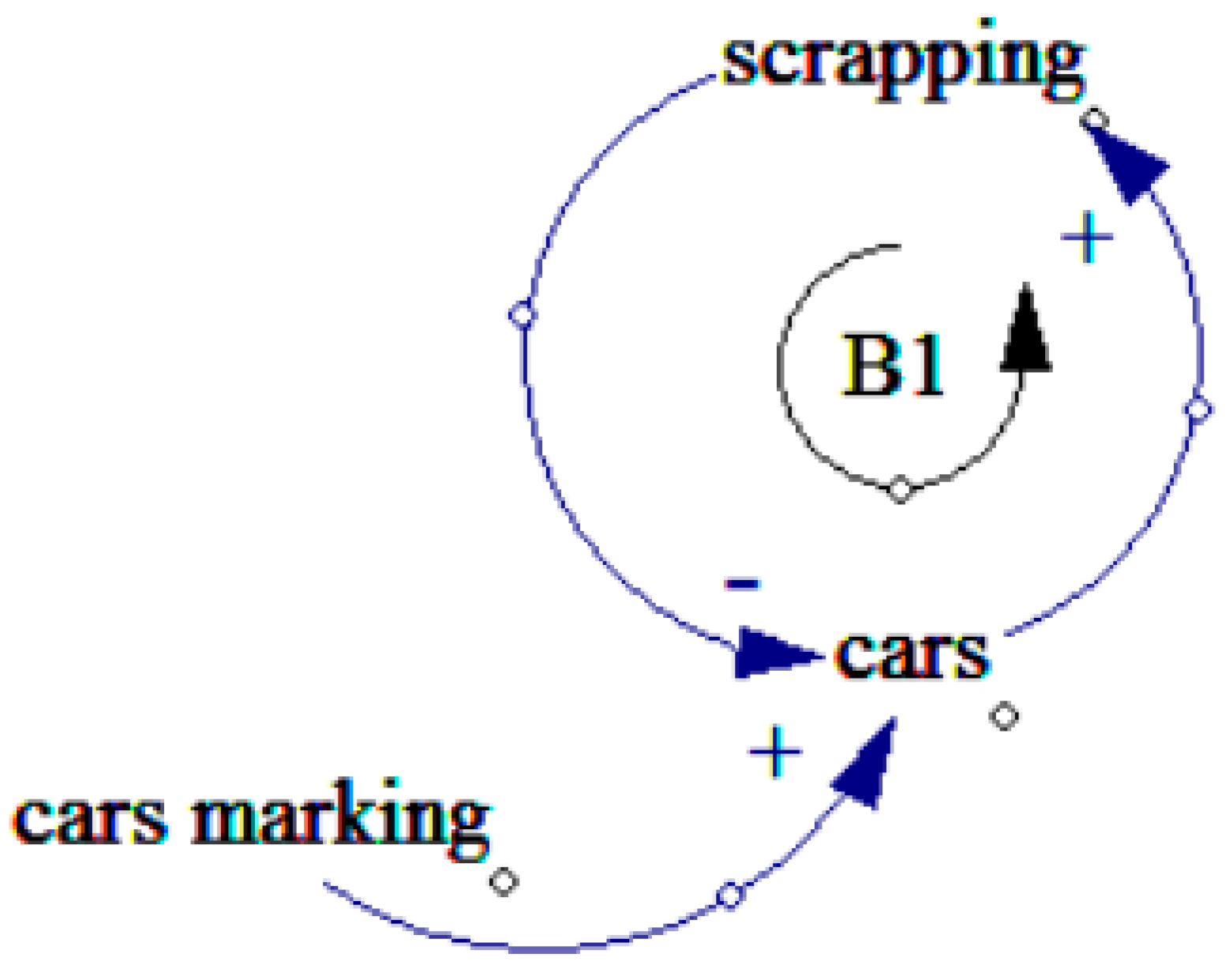
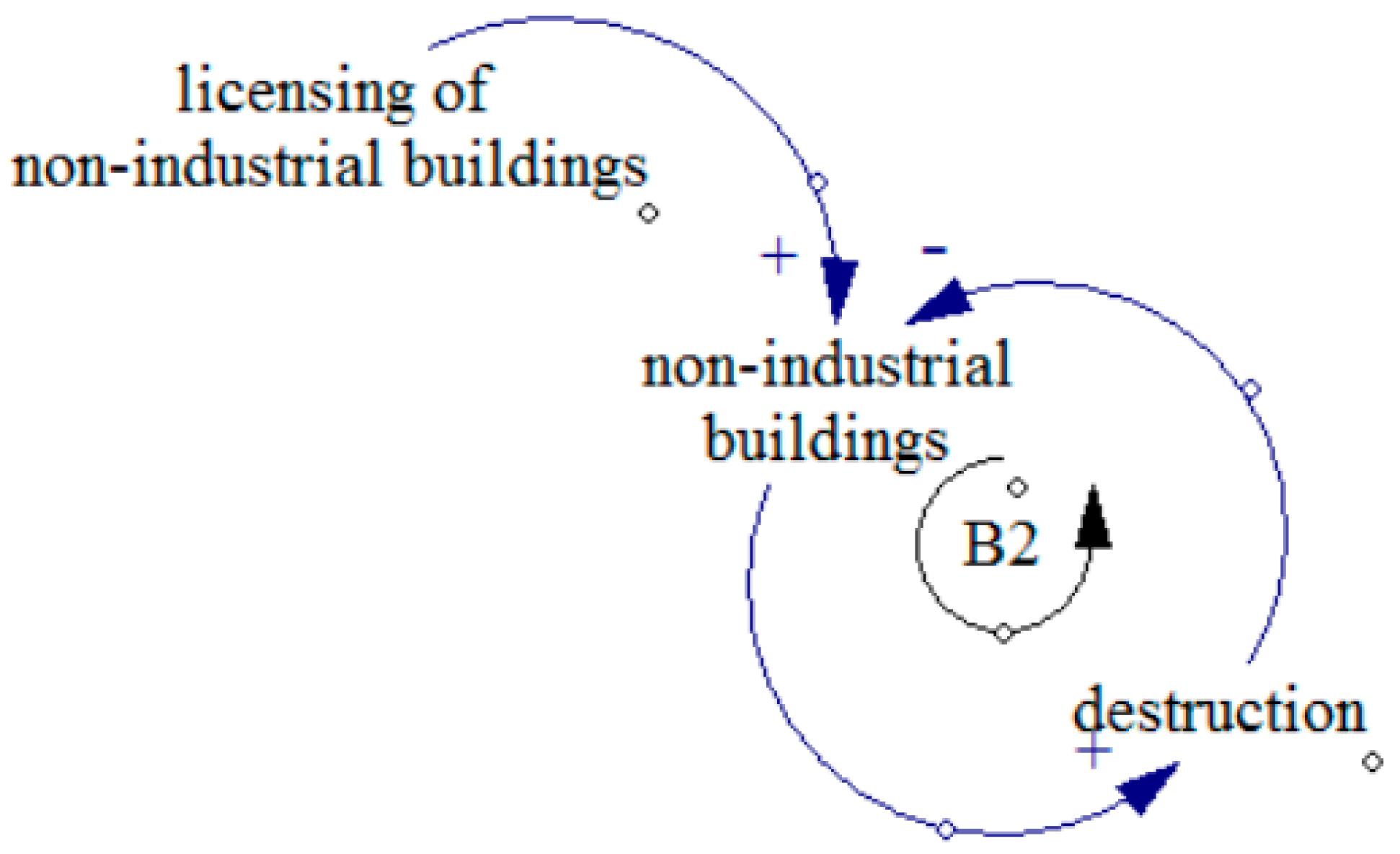
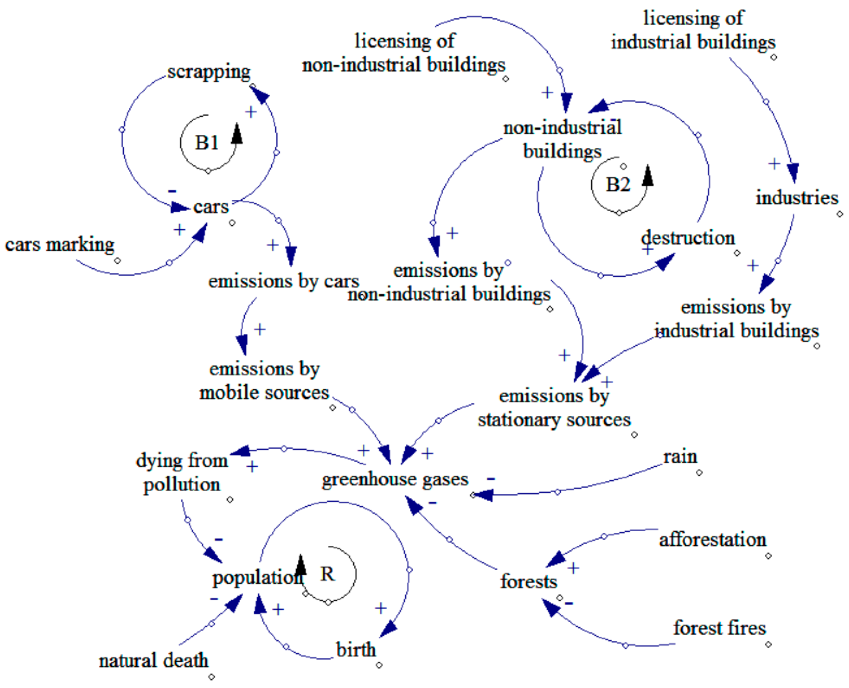
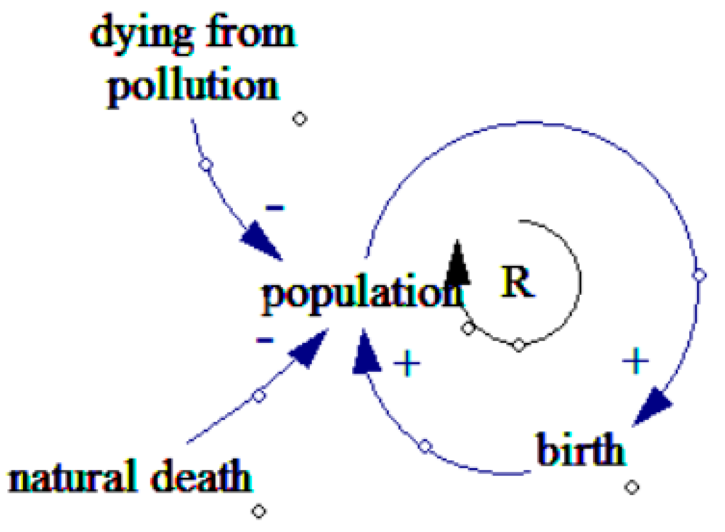
• Stage 2. Drawing a causal loop diagram for the system of greenhouse gases emissions in Tehran.
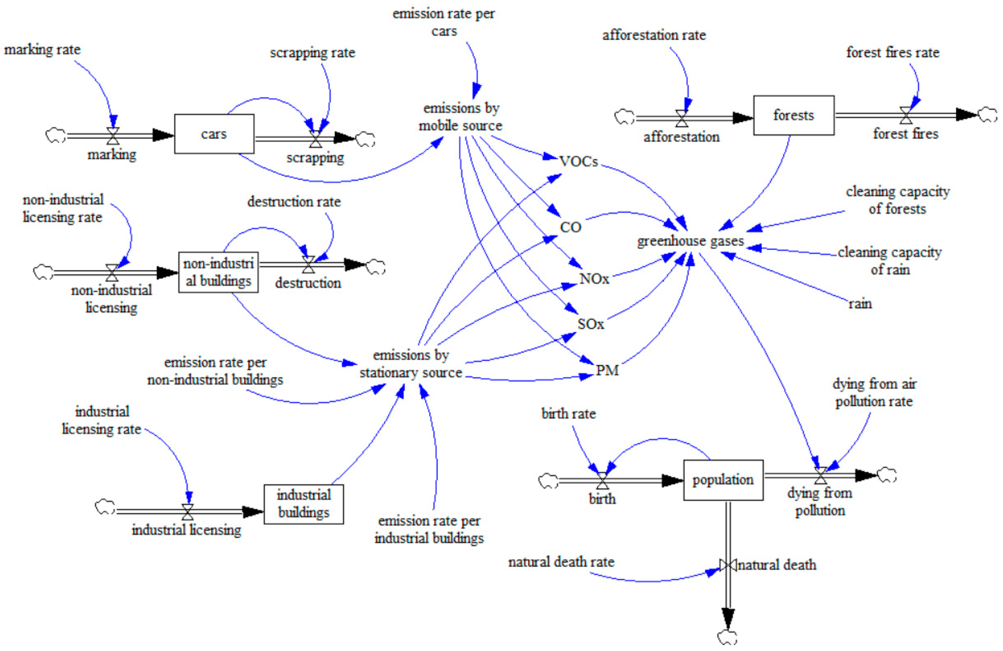
• Stage 3. Drawing a stock-flow diagram of the system of greenhouse gases emissions in Tehran.
• Stage 4. Compiling and formulating a model of the system of greenhouse gas emissions in Tehran in mathematical form, which shows interactions inside the system.
• Stage 5. Identifying critical variables through the statistical method of design of experiments.
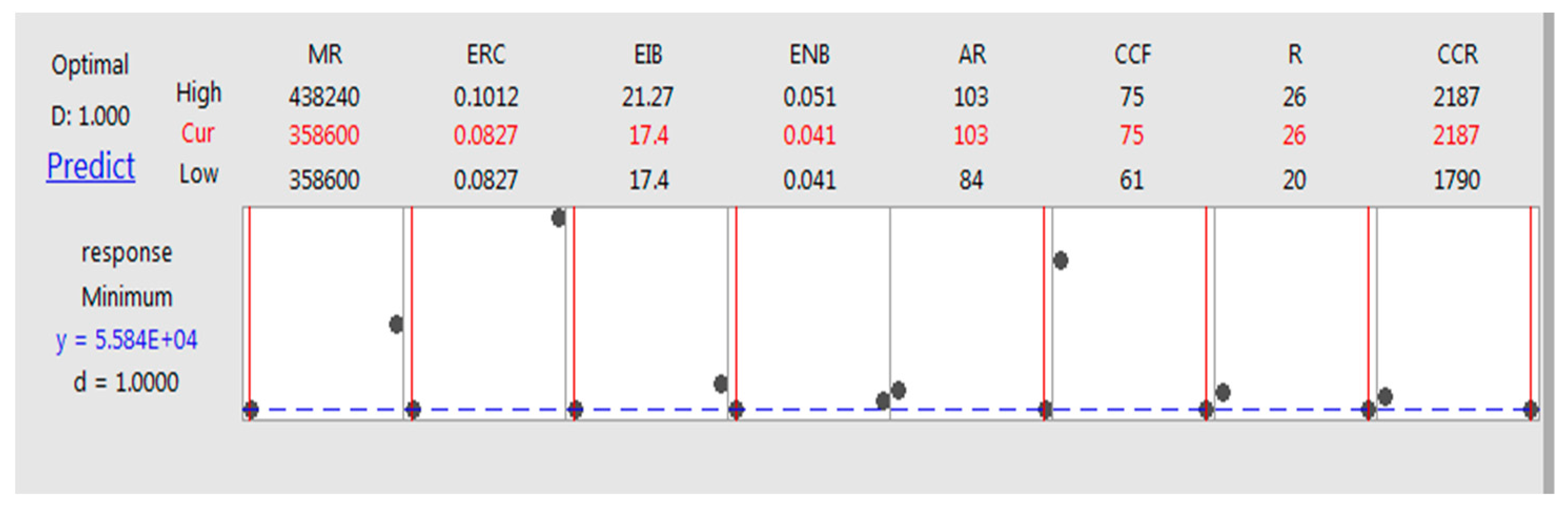
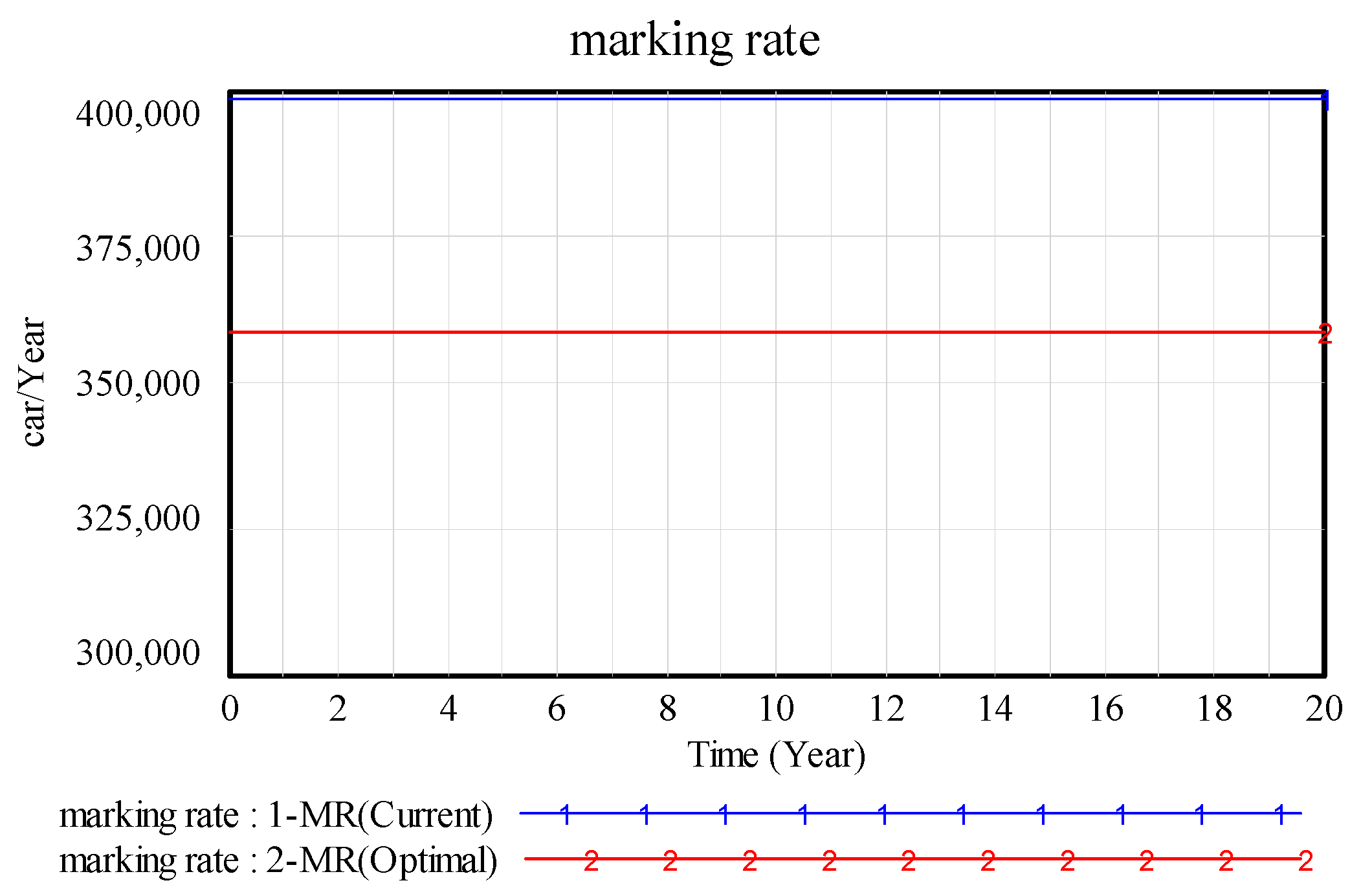
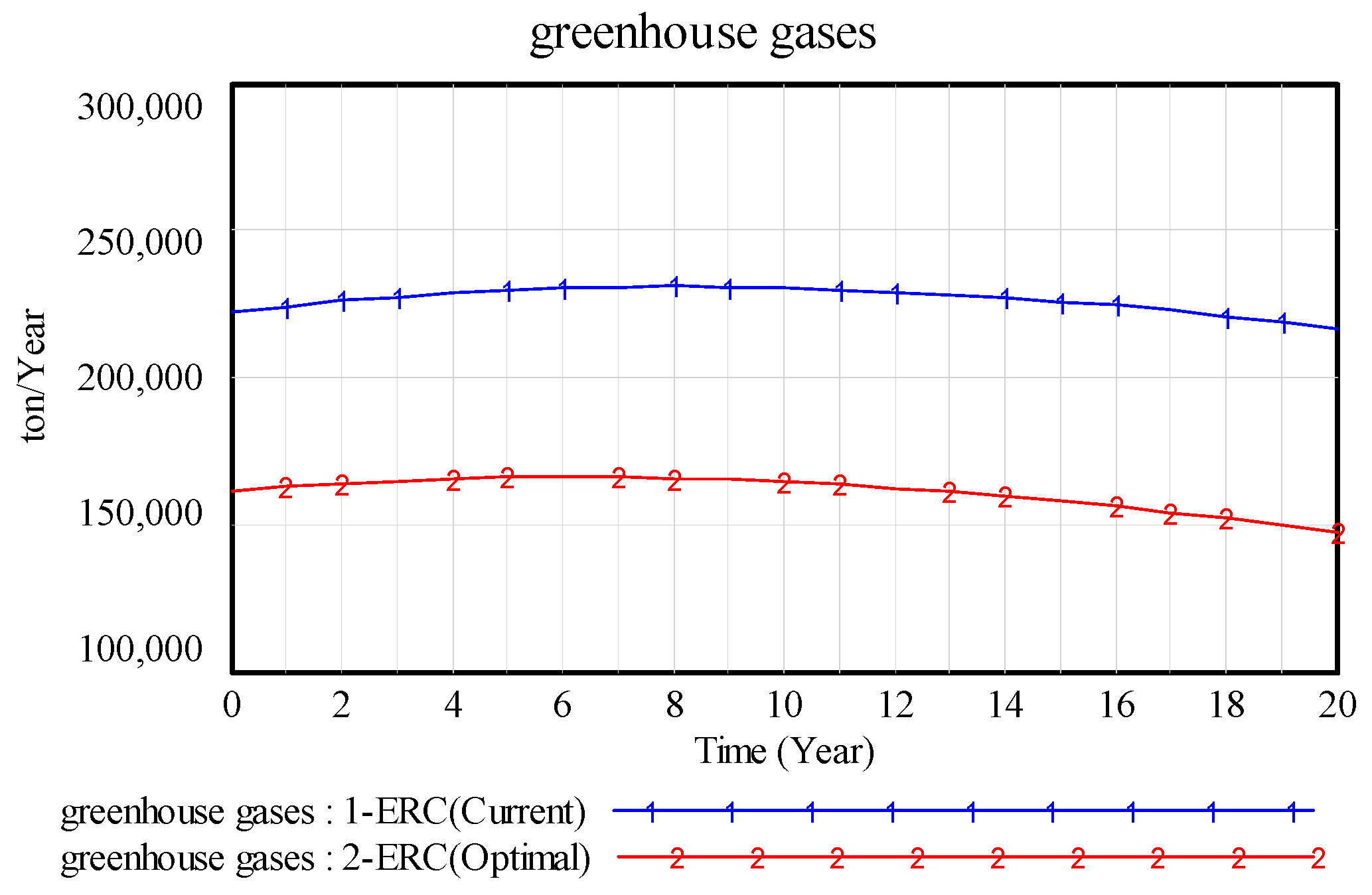
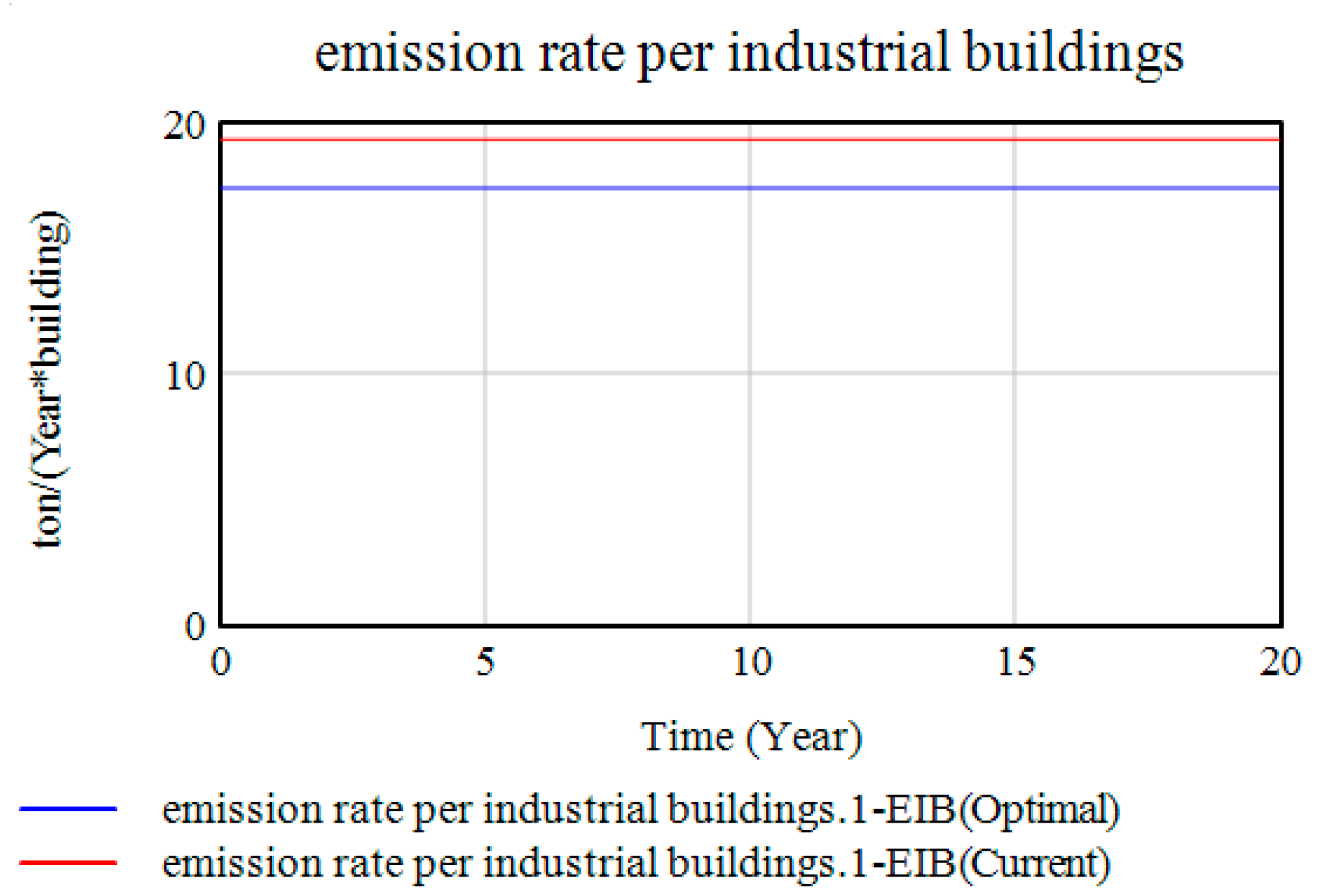
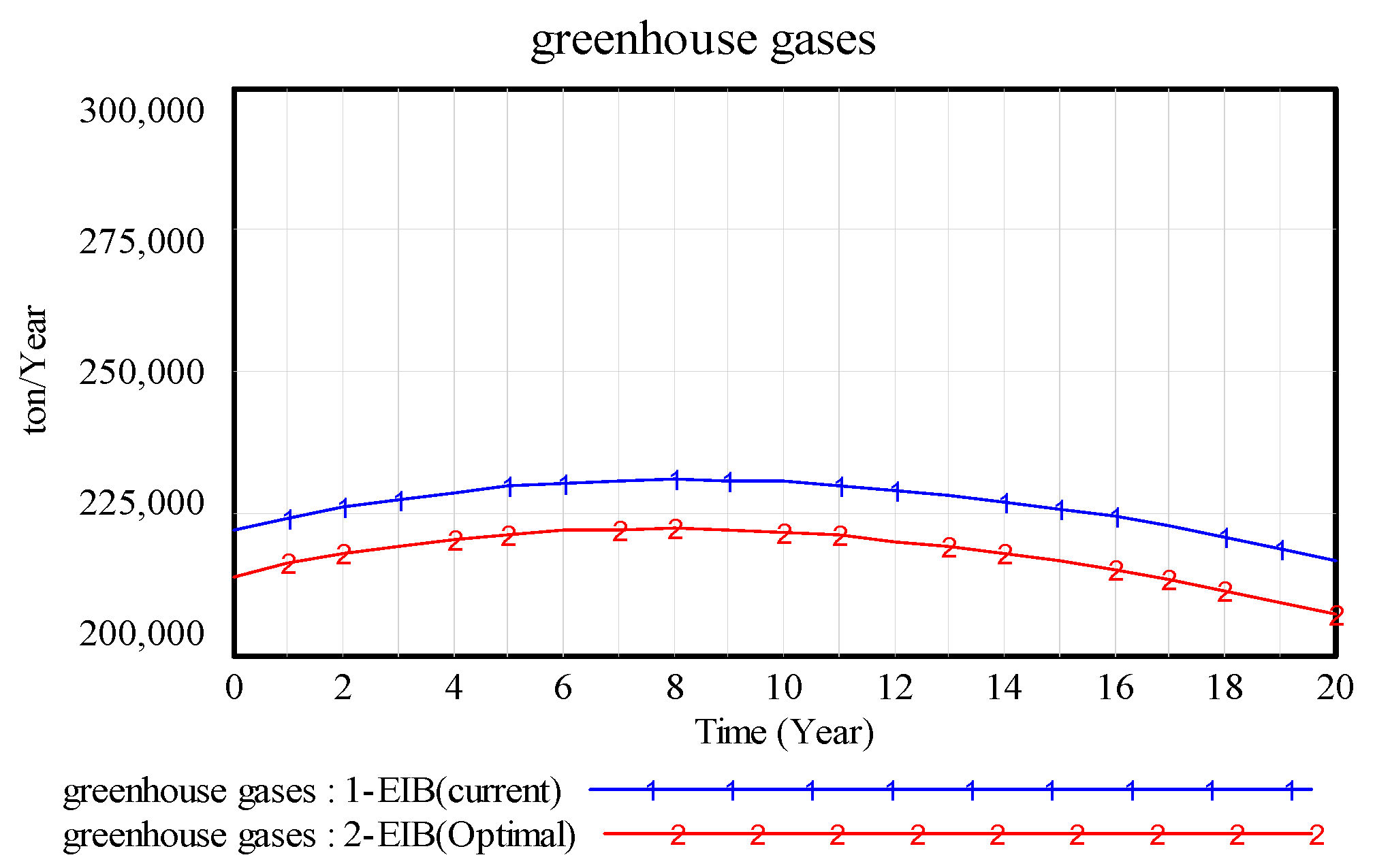
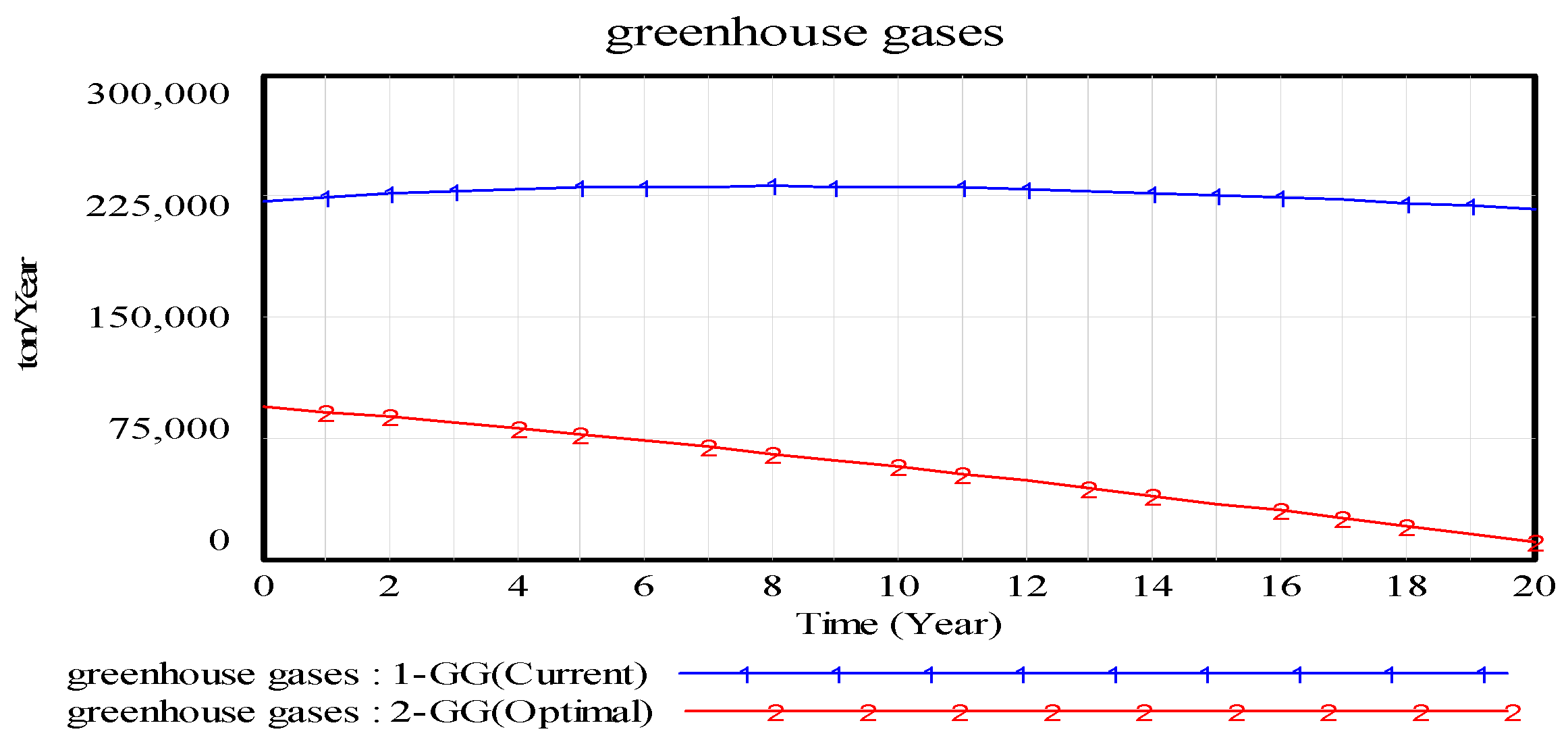
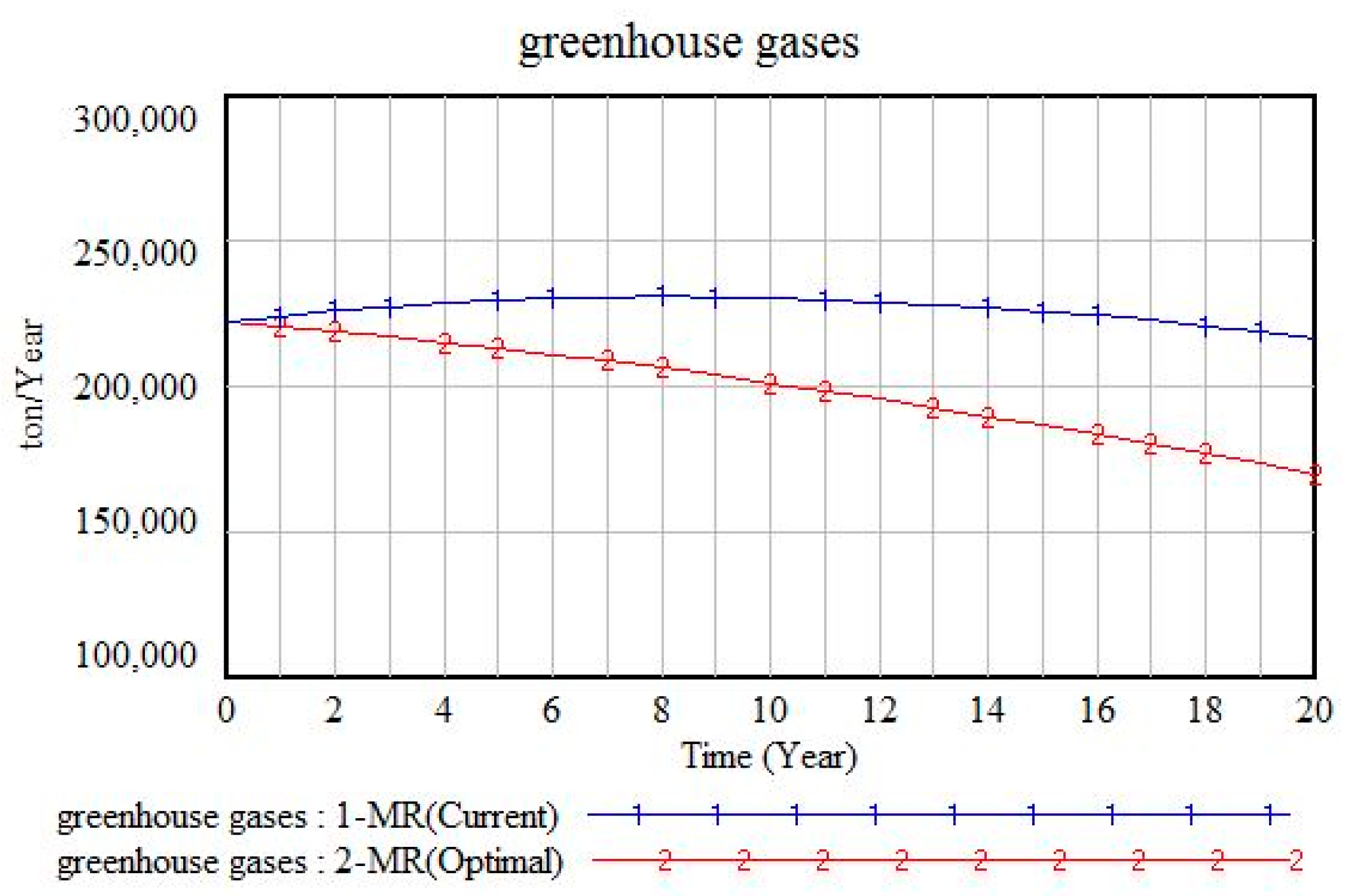
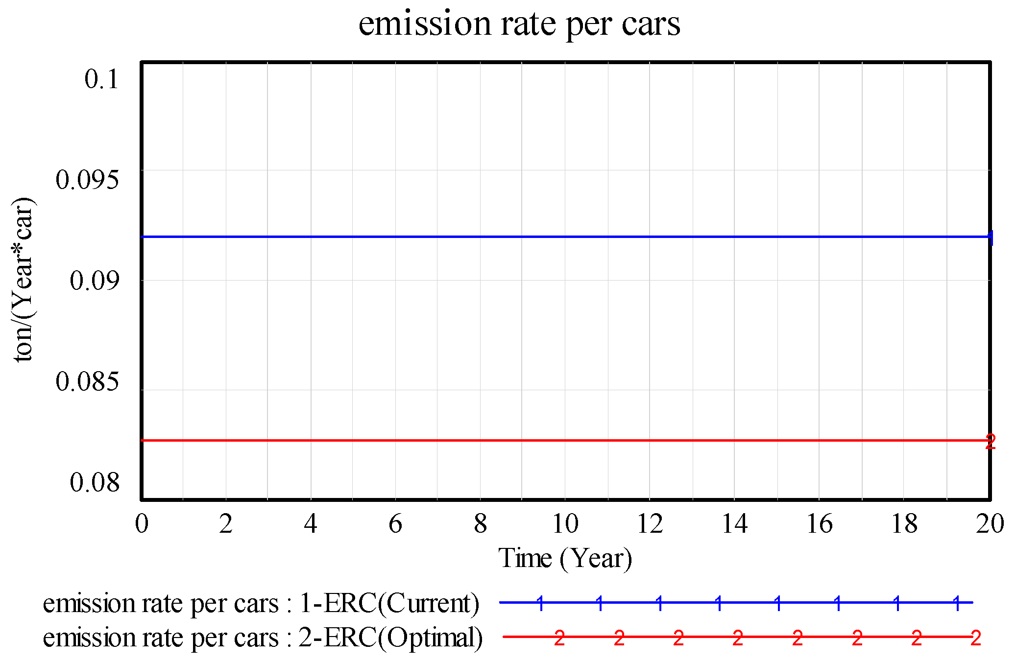
• Stage 6. Demonstrating the output of the model based on optimal values.
• Stage 7. Defining scenarios for reducing greenhouse gases based on optimized values.

Data for this model were collected from government sites and the model was constructed using causal loops designed based on dynamic hypotheses defined by field experts. Further details pertaining to the data can be found in the Appendix A.

2.1. Causal Loop Diagram

The causal loop diagram is a simple map which shows the relations between the variables by means of arrows relating the cause to the effect. Additionally, the causal loop diagram is a system theory loop which is composed of two balance and reinforcement circles. In the causal loop diagram, the arrows with a mark of “+” are used for the direct relationship between causal loop and those with a minus mark “−” are applied for an inverse relation between causal loop [18].

This article represents Tehran’s air pollution in three loops which will be discussed below. It is necessary to first explain the micro-loops to demonstrate the causal loop diagram. That is why micro-loops are brought forward initially and then the causal loop diagram of the entire system will be illustrated. The diagram in Figure 1 represents the causal diagram of the cars which increases once the number of cars grows. Once the cars are totally gone out of the order (junk or scrapped cars) annually, the number of cars reduces.

Figure 2 demonstrates the circle of a number of non-industrial units in which the units grow once the constructions get a license to expand. After their lifetime, a period of 20 years, they suffer total damage and get out of the circle.

Figure 3 illustrates the circle of population variable; when the birth rate increases the population increases. It reduces by natural death and mortality due to pollution.

Figure 4 shows a causal loop diagram for the whole system. As demonstrated, pollution grows when the pollutants are dispersed. In fact, some of them are destroyed as a result of natural factors and the remaining causes’ deaths.

2.2. Stock-Flow Diagram

Although the causal loop diagrams involve many benefits, in some situations, they also have weaknesses such as the inability to show the stock-flows of the system. This is why stock-flows along with feedback are two central concepts in system dynamics theory.

The stock-flow diagram includes three basic elements: stock, flow, and converters [18]. Stocks suggest accumulations inside the system and its stagnation. Flows indicate stocks deviations for input and output. Finally, converters are auxiliary variables to better visualize variables and adjust flows behaviors [18].

The boxes in the diagram represent stock variables and faucets show input and output flows. Auxiliary variables are marked with no sign in the graph and are simply represented with their own names. To draw the stock-flow diagram, its variables are first presented in

Table 2. Variable units of air pollution stock-flow.

Variable	Unit
MR: Marking rate	car/year
M: Marking	car/year
C: Cars	car/year
S: Scrapping	car
SR: Scrapping rate	1/year
ERC: Emission rate per car	ton/car/year
EMS: Emissions by mobile source	ton/year
NLR: Non-industrial licensing rate	building/year
NL: Non-industrial licensing	building/year
NB: Non-industrial buildings	building
DR: Destruction rate	1/year
D: Destruction	building/year
ENB: Emission rate per non-industrial building	ton/building/year
ILR: Industrial licensing rate	building/year
IL: Industrial licensing	building/year
IB: Industrial buildings	building
EIB: Emission rate per industrial building	ton/building/year
ESS: Emission by stationary sources	ton/year
VOCs	ton/year
CO	ton/year
NOx	ton/year
Sox	ton/year
PM	ton/year
GG: Greenhouse gas	ton/year
AR: Afforestation rate	hectare/year
A: Afforestation	hectare/year
F: Forests	hectare
FFR: Forest fire rate	hectare/year
FF: Forest fire	hectare/year
CCF: Cleaning capacity of forests	ton/hectare/year
R: Rain	day/year
CCR: Cleaning capacity of rain	ton/day/year
BR: Birth rate	1/year
B: Birth	person/year
POP: population	person
DR: Death rate	person/year
ND: Natural death	person/year
DP: Dying from pollution	person/year
DPR: Dying from air pollution rate	person/ton

. Then, in Figure 5, the diagram is presented.

2.3. Compiling and Formulating the Model and Developing a Mathematical Method

Data were collected from a variety of sources to compile and formulate the variables; the references are provided in

Table A1. Sources of collected data.

Variable	Source	Website Address and References
Cars	Analytical website of Asr-e Iran, 1394 (2015)	www.asriran.com [26] (accessed on 20 October 2021).
Rate	Tehran statistical yearbook (Statistics website)	www.amar.org.ir [27] (accessed on 20 October 2021).
Non-industrial buildings	Statistics inference of Tehran municipality 2007–2011 mean 25	www.tehran.ir [28] (accessed on 20 October 2021).
Non-industrial licensing rate	Tehran municipality website	www.tehran.ir [28] (accessed on 20 October 2021).
Destruction rate	Question from expert	-
Industrial buildings	Tehran Industrial, Mining, and Trade Organization	www.teh.mimt.gov.ir [29] (accessed on 20 October 2021).
Industrial licensing rate	Tehran municipal website	www.tehran.ir [28] (accessed on 20 October 2021).
GG + VOCs + CO + NOx + Sox + PM	Tehran pollutant emission inventory 2013	[25]
Emission rate per cars	Based on emission inventory and the number of cars in 2013	[25]
Emission rate per industrial buildings	Based on emission inventory and number of industrial buildings, 2013	[25]
Emission rate per non-industrial buildings	Based on emission inventory and number of non-industrial buildings, 2013	[25]
Forests	Tehran statistics yearbook	www.amar.org.ir [27] (accessed on 20 October 2021).
Afforestation rate	Tehran statistics yearbook	www.amar.org.ir [27] (accessed on 20 October 2021).
Forest fires	Tehran statistics yearbook	www.amar.org.ir [27] (accessed on 20 October 2021).
Cleaning capacity of forests	Iran’s students news agency (ISNA)	www.gilan.isna.ir [30] (accessed on 20 October 2021).
Rain	Tehran statistics yearbook, geophysical station	www.amar.org.ir [27] (accessed on 20 October 2021).
Cleaning capacity of rain	Based on the statistics of daily emission inventory	[25]
Population	Tehran statistics yearbook	www.amar.org.ir [27] (accessed on 20 October 2021).
Birth rate	Tehran statistics yearbook	www.amar.org.ir [27] (accessed on 20 October 2021).
Natural death	Tehran statistics yearbook	www.amar.org.ir [27] (accessed on 20 October 2021).
Dying from pollution	Islamic republic pf Iran’s news agency (IRNA), compared to pollution in 2013	www.irna.ir [31]

in Appendix A.

The model contains five stock variables defined using the following Equations:

C = INTEG (M-S, 6,534,000)

(1)

M = MR

(2)

MR = 398,399

(3)

S = C*SR

(4)

SR = 1/20

(5)

EMS = C*ERC

(6)

ERC = 0.0919765

(7)

NL = BR

(8)

NL = BR

(9)

NLR = 31,091.5

(10)

D = DR*NB

(11)

DR = 1/25

(12)

IB = INTEG (IL, 4075)

(13)

IL = ILR

(14)

ILR = 48

(15)

ESS = (EIB*IB) + (ENB*NB)

(16)

EIB = 19.341

(17)

ENB = 0.046036

(18)

VOCs = ((71,944/613,834)*EMS) + ((11,696/107,927)*ESS)

(19)

Co = ((494,201/613,834)*EMS) + ((12,489/107,927)*ESS)

(20)

NOx = ((39,430/613,834)*EMS) + ((46,094/107,927)*ESS)

(21)

Sox = ((2326/613,834)*EMS) + ((35,085/107,927)*ESS)

(22)

PM = ((5933/613,834)*EMS) + ((2563/107,927)*ESS)

(23)

GG = (CO + NOx + PM + Sox + VOCs) − ((CCF*F)+(CCR*R))

(24)

F = INTEG (A − FF, 6452)

(25)

A = AR

(26)

AR = 93.583

(27)

FF = FFR

(28)

FFR = 10.25

(29)

CCF = 68

(30)

R = 23

(31)

CCR = 1989

(32)

POP = INTEG (B-ND-DP, 8.29314 × 10⁶)

(33)

B = BR*POP

(34)

BR = 0.014616

(35)

ND = DR

(36)

DR = 39,317

(37)

DP = PO*DPR

(38)

DPR = 1/51.318

(39)

Note that the first stock variable denotes the number of cars and Equation (1) represents this number in 2011. Equation (2) represents the input flow to the car variable, which is equal to the rate of cars per year. The corresponding number in 2011 is represented by Equation (3). Equation (4) represents the car stock which equals the number of cars multiplied by the rate of scrapped (or junk) cars. The corresponding value in 2011 is represented by Equation (5). Equation (6) depicts the amount of pollutants generated by cars which is the number of cars multiplied by the pollution rate of each car, the value in 2011 of which is given by Equation (7). Equally, Equation (8) relates to the stock variable of non-industrial buildings along with the corresponding value in 2011. Equation (9) shows the input variable of non-industrial buildings which equals the number of issued licenses and permits per year. The corresponding value in 2011 is given in Equation (10). Equation (11) shows the output variable of non-industrial buildings, i.e., the number of buildings multiplied by the rate of their destruction. The corresponding value for our case study is given in Equation (12). Equation (13) indicates the number of industrial buildings. Equation (14) indicates the number of industrial construction permits per year. The corresponding value for our case study is given in Equation (15). Equation (16) represents the amount of greenhouse gas emissions by stationary sources which is equal to the amount of greenhouse gases emitted by industrial and non-industrial buildings. Equations (17) and (18) depict the rate of greenhouse gas emissions by industrial and non-industrial constructions, respectively. Equation (19) through Equation (23) provide the amount of greenhouse gases from mobile and stationary emission sources each (cars and buildings). Equation (24) provides the sum of all greenhouse gases. Equation (25) represents the stock variable of forests along with its corresponding value in 2011. Equation (26) represents forestry rate per year, whose value in 2011 is depicted in Equation (27). Equation (28) represents the forests fires per year. The corresponding value in 2011 is given in Equation (29). Equation (30) provides the rate of greenhouse gases cleaned by one hectare of forest. Equations (31) and (32) respectively show the number of rainy days per year as well as the rate of cleaning greenhouse gases on one rainy day. Equation (33) represents the city’s population along with its value in 2011. Equation (34) illustrates the population growth computed by multiplying the population rate by birth rate. Its corresponding value in 2011 is given by Equation (35). Equation (36) represents the number of deaths (death toll) of the first output flow variable of the population. This rate for our study is given by Equation (37). Equation (38) shows the second output variable of the population (death rate as a result of pollutants), indicating the number of deaths due to pollution, whose amount equals the amount of pollutants by the pollutant rate that can result in one death. Its value for our case study is given by Equation (39).

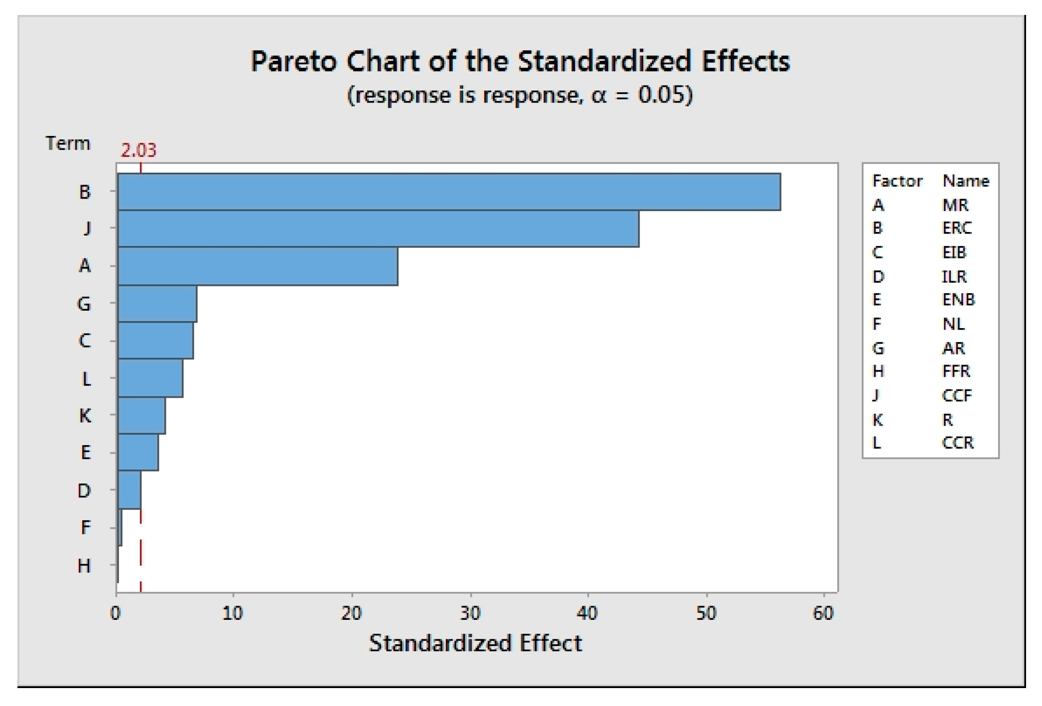
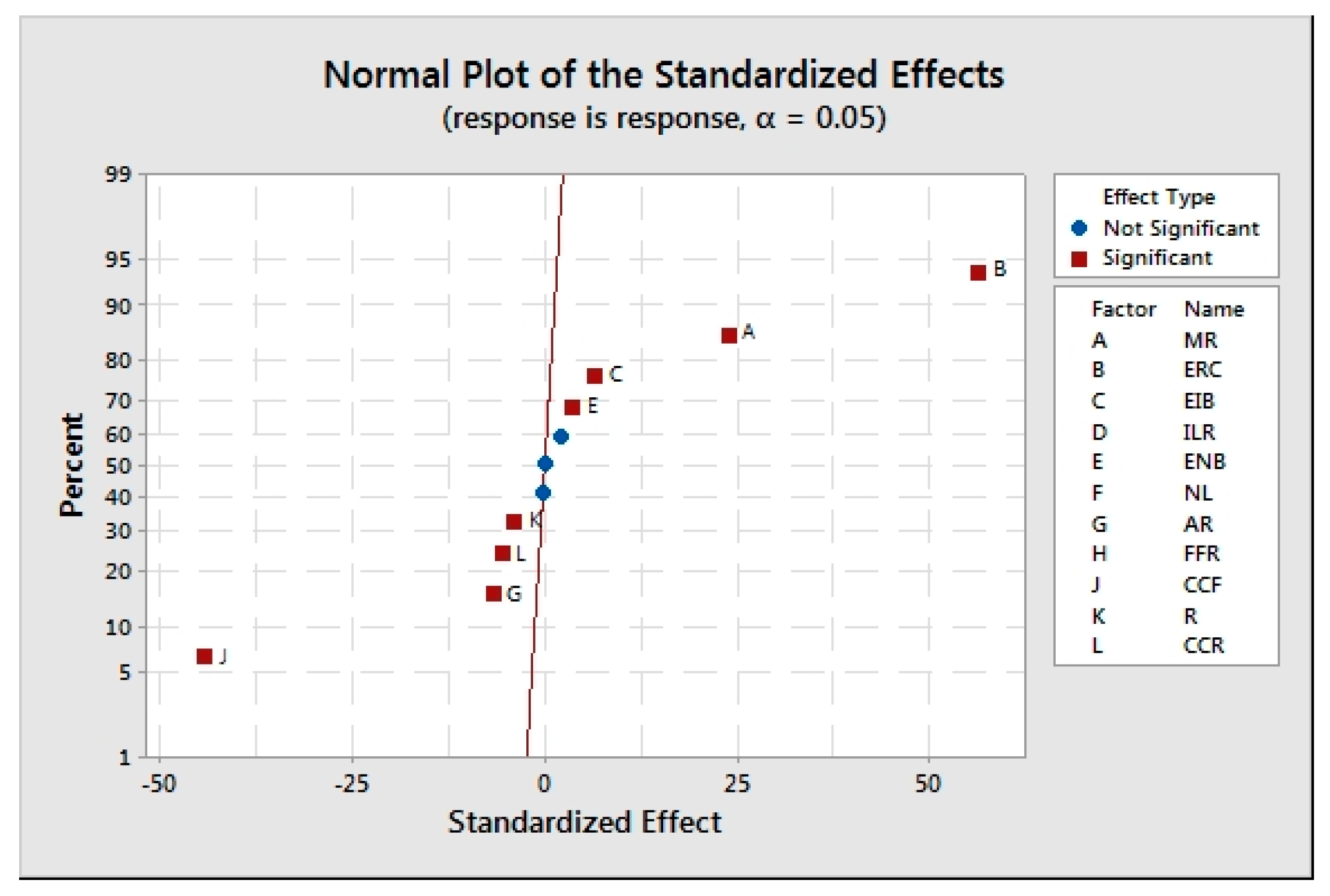
2.4. Identifying Major Variables and Improving Them by Design of Experiments (DoE)

The statistical method of design of experiments was carried out using the Minitab software version 17.3.1. The main variables were identified as follows:

• Eight variables out of eleven were identified using the factorial design of Plackett–Burman.
• The eight variables were entirely tested. The corresponding uppermost and lowermost rates for these variables are illustrated in

  Table 3. The high and low rates of each variable.

  Variable	Lowermost Rate	Uppermost Rate
  MR	358,600	438,240
  ERC	0.0827	0.1012
  ILR	43	52
  EIB	17.4	21.27
  ENB	0.041	0.051
  NL	27,982	34,200
  AR	84	103
  FFR	9	12
  CCF	61	75
  R	20	26
  CCR	1790	2187

  .

To design the experiments of the first stage, which was of Plackett–Burman, the following path was followed in Minitab software.

Stat→DoE→Factorial→Create Factorial Design→Plackett–Burman design

Figure 6 depicts the results of 48 experiments carried out in the first stage.

As represented in Figure 6 and Figure 7, eight variables were identified for marking cars, greenhouse gas emission rate of each car, greenhouse gas emission rate of each industrial building, greenhouse gas emission rate of each non-industrial unit, as well as forestry, cleaning rate of per hectare of forest, raining, and air cleaning rate of rain, which were the major pollution system’s variables.

Figure 8 indicates the optimized amount of each variable to reduce pollution.

Entering each amount, the existing greenhouse gas emission in the air reached 0.0005584 tons per year. Different scenarios were defined based on the amounts. To do this, the optimal amount of each variable was entered in the stock-flow diagram and then the effect of the same variable, and finally, the amount of greenhouse gas emissions was observed. Finally, the optimal amounts of all variables were entered into the model and their entire effect was examined on the amount of greenhouse gases.

3. Results and Discussion

In this research, the model was run for 20 years (from 2011 to 2031). First, data from 10 years ago were given to the model then the actual results were compared with the model results in the first 10 years (2011–2021). The results were almost similar. Therefore, the results of the model in the next 10 years (2021–2031) can be trusted.

For performance analysis, the optimal values from Figure 8 were compared to the current and optimal status of three important variables (marking rate, emission rate of car, and emission rate of industrial buildings). Additionally, depending on the variables’ status, their behavior reasons, scenarios, and strategies were discussed.

Figure 9 indicates the rate of car marking based on the current and optimal rates and Figure 10 shows the impact of current and optimal car rate on the amount of greenhouse gas emissions. In the figures, number 1 shows current status, number 2 shows the optimal status of the greenhouse gases amount, and time (0) refers to 2011. Cars are the major source of greenhouse gas emissions in cities. On the other hand, their excessive increase not only increases the air pollution in the cities but it also affects other problems of the cities such as traffic jams, accidents, and so on. Therefore, it is recommended that the car rate be reduced to reduce air pollution and other urban problems. If this is not possible, it is a good idea to scrap the worn-out cars at a higher rate.

Figure 11 depicts the greenhouse gas emissions of each car based on current and optimal rates. Figure 12 shows the effect of greenhouse gas emission rates by each car on the current and optimal amount of greenhouse gas emissions.

Based on the above results, we can conclude that the best strategy to reduce air pollution in cities is to reduce greenhouse gas emissions by cars since (1) cars are traveling on city roads (even on off working days), (2) the most fossil fuels in the cities are consumed by cars, and (3) they are inside the cities whereas factories are located outside. Additionally, manufacturing low emission and environmentally friendly cars can drastically reduce greenhouse gas emissions.

Figure 13 and Figure 14 represent greenhouse gas emissions by industrial buildings and the effect of their optimal and current amount on greenhouse gases emissions, respectively.

As shown by the above figures, greenhouse gas emissions by industrial units are considered one of the sources which generate pollutants. Note, however, that although greenhouse gas emissions by an industrial building are much more than mobile sources, their effect is less, since the number of industrial buildings in cities is negligible compared to the number of cars (approximately 1/1000). On the other hand, industrial units stop generating pollutants when they are closed during holidays and weekends whereas cars never stop moving and generating greenhouse gases.

Figure 15 depicts the amount of greenhouse gas emissions provided by the model when all major and critical variables are at their optimal levels.

The above figure shows a huge a drop in greenhouse gas emissions when the major and critical variables are at their optimum values. Those results confirm the importance of optimizing all major and critical variables to drastically reduce greenhouse gas emissions. It is worth noting, however, that whereas certain variables such as EMS can be optimized using a set of strategies and proper planning, others, such as EIB and ENB, cannot in a well-established urban setting.

4. Conclusions

This paper proposed a simulation model of the air pollution levels in the capital city of Tehran. The model considered air pollution sources and outcomes based on system dynamics. Its aim was to devise strategies to mitigate air pollution for the city of Tehran. The dynamics analysis and obtained results showed that the leading cause of pollution in cities is greenhouse gas emissions. Thus, the best strategy to reduce air pollution is to reduce greenhouse gas emissions by cars since first, cars are traveling on city roads, second, the most fossil fuels in the cities are consumed by the cars, and third, they are inside the cities whereas factories are located outside. Hence, manufacturing environmentally friendly cars which can rely on renewable energy resources as their fuels can provide a viable solution to reduce air pollutants. The other highly important strategy is to preserve forests which are the most valuable resources after water and air, they are countries’ wealth for a better life. Additionally, strategies aiming at reducing pollution by industrial units should also be considered. It should be noted that avoiding environmental pollution is better and cheaper than cleaning up or mitigating the impact of pollution.

Future works can focus on developing similar models based on data collected from other countries and draw global solutions to the pollution problem.

References

1. Kokkos, N.; Zoidou, M.; Zachopoulos, K.; Nezhad, M.; Garcia, D.; Sylaios, G. Wind Climate and Wind Power Resource Assessment Based on Gridded Scatterometer Data: A Thracian Sea Case Study. Energies 2021, 14, 3448. [Google Scholar] [CrossRef]
2. Razmjoo, A.; Khalili, N.; Nezhad, M.M.; Mokhtari, N.; Davarpanah, A. The main role of energy sustainability indicators on the water management. Model. Earth Syst. Environ. 2020, 6, 1419–1426. [Google Scholar] [CrossRef] [Green Version]
3. Mayer, H. Air pollution in cities. Atmos. Environ. 1999, 33, 4029–4037. [Google Scholar] [CrossRef]
4. Flagan, R.C.; Seinfeld, J.H. Fundamentals of Air Pollution Engineering; Dover Publication Inc.: New York, NY, USA, 2012. [Google Scholar]
5. Miri, M.; Derakhshan, Z.; Allahabadi, A.; Ahmadi, E.; Conti, G.O.; Ferrante, M.; Aval, H.E. Mortality and morbidity due to exposure to outdoor air pollution in Mashhad metropolis, Iran. The AirQ model approach. Environ. Res. 2016, 151, 451–457. [Google Scholar] [CrossRef] [PubMed]
6. Okedere, O.B.; Olalekan, A.P.; Fakinle, B.S.; Elehinafe, F.B.; Odunlami, O.A.; Sonibare, J.A. Urban air pollution from the open burning of municipal solid waste. Environ. Qual. Manag. 2019, 28, 67–74. [Google Scholar] [CrossRef]
7. Daly, A.; Zannetti, P. An Introduction to Air Pollution–Definitions, Classifications, and History. Available online: https://www.nile-center.com/uploads/RQZG7BCW4DGXNSZ.pdf (accessed on 20 October 2021).
8. Chandna, A.; Honney, R. INSPiRE: An integrated approach to tackling household air pollution and improving health in rural Cambodia. Public Health 2017, 145, 70–74. [Google Scholar] [CrossRef] [PubMed]
9. Dziubanek, G.; Spychała, A.; Marchwińska-Wyrwał, E.; Rusin, M.; Hajok, I.; Ćwieląg-Drabek, M.; Piekut, A. Long-term exposure to urban air pollution and the relationship with life expectancy in cohort of 3.5 million people in Silesia. Sci. Total Environ. 2017, 580, 1–8. [Google Scholar] [CrossRef] [PubMed]
10. Fu, S.; Gu, Y. Highway toll and air pollution: Evidence from Chinese cities. J. Environ. Econ. Manag. 2017, 83, 32–49. [Google Scholar] [CrossRef] [Green Version]
11. Gillespie, J.; Masey, N.; Heal, M.R.; Hamilton, S.; Beverland, I.J. Estimation of spatial patterns of urban air pollution over a 4-week period from repeated 5-minute measurements. Atmos. Environ. 2016, 150, 295–302. [Google Scholar] [CrossRef]
12. Hassan, S.K.; Khoder, M.I. Chemical characteristics of atmospheric PM 2.5 loads during air pollution episodes in Giza, Egypt. Atmospheric Environ. 2017, 150, 346–355. [Google Scholar] [CrossRef]
13. Albin, S.; Forrester, J. Building a System Dynamics Model. Available online: https://ocw.mit.edu/courses/sloan-school-of-management/15-988-system-dynamics-self-study-fall-1998-spring-1999/readings/building.pdf (accessed on 20 October 2021).
14. Todorov, V.; Ostromsky, T.; Dimov, I.; Georgieva, R. Optimized Stochastic Methods for Sensitivity Analysis for Large-Scale Air Pollution Model. Available online: https://annals-csis.org/Volume_26/drp/pdf/51.pdf (accessed on 20 October 2021).
15. Artun, G.K.; Polat, N.; Yay, O.D.; Üzmez, Ö.Ö.; Arı, A.; Tuygun, G.T.; Elbir, T.; Altuğ, H.; Dumanoğlu, Y.; Döğeroğlu, T.; et al. An integrative approach for determination of air pollution and its health effects in a coal fired power plant area by passive sampling. Atmospheric Environ. 2017, 150, 331–345. [Google Scholar] [CrossRef]
16. Dakos, V.; Soler-Toscano, F. Measuring complexity to infer changes in the dynamics of ecological systems under stress. Ecol. Complex. 2017, 32, 144–155. [Google Scholar] [CrossRef]
17. Ossimitz, G.; Mrotzek, M. The basics of system dynamics: Discrete vs. continuous modelling of time. In Proceedings of the 26th International Conference of the System Dynamics Society Athens/Greece, Athens, Greece, 20–24 July 2008; pp. 1–8. [Google Scholar]
18. Todorov, V.; Dimov, I.; Ostromsky, T.; Apostolov, S.; Georgieva, R.; Dimitrov, Y.; Zlatev, Z. Advanced stochastic approaches for Sobol’ sensitivity indices evaluation. Neural Comput. Appl. 2021, 33, 1999–2014. [Google Scholar] [CrossRef]
19. Cheng, L.I. System dynamics model of Suzhou water resources carrying capacity and its application. Water Sci. Eng. 2010, 3, 144–155. [Google Scholar]
20. Wei, S.; Yang, H.; Song, J.; Abbaspour, K.C.; Xu, Z. System dynamics simulation model for assessing socio-economic impacts of different levels of environmental flow allocation in the Weihe River Basin, China. Eur. J. Oper. Res. 2012, 22, 248–262. [Google Scholar] [CrossRef]
21. Yu, S.; Wang, K.; Wei, Y.-M. A hybrid self-adaptive Particle Swarm Optimization–Genetic Algorithm–Radial Basis Function model for annual electricity demand prediction. Energy Convers. Manag. 2015, 91, 176–185. [Google Scholar] [CrossRef]
22. Chaves, R.; López, D.; Macías, F.; Casares, J.; Monterroso, C. Application of System Dynamics technique to simulate the fate of persistent organic pollutants in soils. Chemosphere 2013, 90, 2428–2434. [Google Scholar] [CrossRef]
23. Bastan, M.; Khorshid-Doust, R.R.; Sisi, S.D.; Ahmadvand, A. Sustainable development of agriculture: A system dynamics model. Kybernetes 2018, 47, 142–162. [Google Scholar] [CrossRef]
24. Montgomery, D.C. Design and Analysis of Experiments; John Wiley & Sons: Hoboken, NJ, USA, 2017. [Google Scholar]
25. Shahbazi, H.; Taghvaee, S.; Hosseini, V.; Afshin, H. A GIS based emission inventory development for Tehran. Urban Clim. 2016, 17, 216–229. [Google Scholar] [CrossRef]
26. Analytical Website of Asr-e Iran. Available online: http://www.asriran.com (accessed on 20 October 2021).
27. Tehran Statistical Yearbook. Available online: http://www.amar.org.ir (accessed on 20 October 2021).
28. Tehran Municipality Website. Available online: http://www.tehran.ir (accessed on 20 October 2021).
29. Tehran Industrial, Mining, and Trade Organization. Available online: http://www.teh.mimt.gov.ir (accessed on 20 October 2021).
30. Iran’s Students News Agency. Available online: http://www.gilan.isna.ir (accessed on 20 October 2021).
31. Islamic Republic pf Iran’s News Agency (IRNA). Available online: http://www.irna.ir (accessed on 20 October 2021).
Figure 1. Cars loop.
Sustainability 14 01181 g001
Figure 2. Non-industrial units loop.
Sustainability 14 01181 g002
Figure 3. Population loops.
Sustainability 14 01181 g003
Figure 4. Causal loop diagram for the climate pollution in Tehran.
Sustainability 14 01181 g004
Figure 5. Stock-flow diagram of Tehran’s air pollution.
Sustainability 14 01181 g005
Figure 6. Pareto diagram of the system’s variables.
Sustainability 14 01181 g006
Figure 7. Normal diagram for identifying the major pollution variables.
Sustainability 14 01181 g007
Figure 8. The optimal amount of each variable.
Sustainability 14 01181 g008
Figure 9. Comparing current and optimal marking rate.
Sustainability 14 01181 g009
Figure 10. The effect of marking rate on the amount of greenhouse gases.
Sustainability 14 01181 g010
Figure 11. Comparing current and optimal cars emission rate.
Sustainability 14 01181 g011
Figure 12. The effect of cars emission rate on the amount of greenhouse gases.
Sustainability 14 01181 g012
Figure 13. Comparing the current and optimal industrial buildings emission rate.
Sustainability 14 01181 g013
Figure 14. The effect of industrial building emission rate on the amount of greenhouse gases.
Sustainability 14 01181 g014
Figure 15. The greenhouse gases status when all critical variables are optimized.
Sustainability 14 01181 g015