Assessment of the Uncertainty Associated with Statistical Modeling of Precipitation Extremes for Hydrologic Engineering Applications in Amman, Jordan

Abstract

Estimates of extreme precipitation are commonly associated with different sources of uncertainty. One of the primary sources of uncertainty in the statistical modeling of precipitation extremes comes from extreme data series (i.e., sampling uncertainty). Therefore, this research aimed to quantify the sampling uncertainty in terms of confidence intervals. In addition, this article examined how the data record length affects predicted extreme precipitation estimates and data set statistics. A nonparametric bootstrap resample was utilized to quantify the precipitation quantile sampling distribution at a particular non exceedance probability. This sampling distribution can provide a point estimation of the precipitation quantile and the confidence interval at a particular non exceedance probability. It has been shown that the different types of probability distributions fit the extreme precipitation data series of various weather stations. Therefore, the uncertainty analysis should be conducted using the best-fit probability distribution for extreme precipitation data series rather than a predefined single probability distribution for all stations based on modern extreme value theory. According to the 95% confidence intervals, precipitation quantiles are subject to significant uncertainty and the band of the uncertainty intervals increases with the return period. These uncertainty bounds need to be integrated into any frequency analysis from historical data. The average, standard deviation, skewness and kurtosis are highly affected by the data record length. Thus, a longer record length is desirable to decrease the sampling uncertainty and, therefore, decrease the error in the predicted quantile values. Moreover, the results suggest that a series of at least 40 years of data records is needed to obtain reasonably accurate estimates of the distribution parameters and the precipitation quantiles for 100 years return periods and higher. Using only 20 to 25 years of data to obtain estimates of the higher return period quantile is risky, since it created high sampling variability relative to the full data length.

1. Introduction

Extreme event statistics are still attracting considerable attention from many researchers around the globe [1,2,3,4,5,6,7]. This is due to the fact of their potential impacts on society and the economy through their importance in the design of various water management infrastructures, water resources modeling and planning, and climate change studies [8,9,10,11]. In Jordan, the 50 and 100 year extreme precipitation events occurred more frequently in recent years, with high precipitation extremes of 106.6–173.8 mm per day for the 50 year return period and 127–194 mm per day for the 100 year return period [6]. Thus, numerous existing water-related infrastructures are at risk due to the fact of aging and possible insufficient consideration of uncertainty when anticipating high precipitation for design purposes. For example, in November 2015, a flash flood in Amman, Jordan, resulting from approximately 45 mm of precipitation over 40 min, causing four deaths and bringing considerable losses to society [6]. In another incident, on 25 October 2018, Jordan’s Dead Sea flash flood killed at least 22 people, mainly schoolchildren and teachers [12,13].

Until now, the frequency analysis concept has widely been considered to be the most essential tool for statistically modeling extreme events. This concept involves selecting and fitting an appropriate probability distribution to the available historical extreme precipitation data [14,15]. From the frequency analysis, extreme precipitation amounts for a given design return period, usually greater than the length of the recorded data series, can be estimated [16]. However, the presence of multiple sources of inadequate accuracies in the frequency analysis process may result in significant uncertainty when predicting extreme precipitation events, resulting in poor design judgments [17,18,19].

Accordingly, the major sources of uncertainties in a precipitation frequency analysis come from the extreme data series, the selection of the frequency distribution, and the parameter estimation methods. The uncertainty associated with the used data set is primarily due to the inaccuracies generated by the insufficiently representative data due to the fact of missing records and the shortness of the recorded length of precipitation in comparison to the return period of the projected extreme precipitation of interest [20,21,22,23]. Additionally, measuring errors owing to instrumental and human error are included, especially when transferring precipitation records from station log files to computers. Another source of uncertainty linked with a used data set is that the observed data set fails to satisfy stationarity and serial independence presumptions [24,25,26]. Stationarity and serial uncorrelation are inherent prerequisite assumptions for the reliability of frequency analysis estimations [24,25,26].

Furthermore, there is also data uncertainty related to the method of sampling the extreme precipitation (i.e., the method of defining extreme precipitation) from a historically observed daily precipitation data set, either as an annual maximum (AM) series or as peaks over a threshold (POT) series. Noteworthy, the differences in the various methods for defining the threshold value when using a POT data series and their impact on the study results present great uncertainty [3,27,28,29].

In the literature, a number of competitive theoretical probability distributions have been available for describing/estimating extreme precipitation amounts in the frequency analysis, and their selection is typically guided by a variety of statistical goodness of fit tests/and the choices among them are generally based on several statistical goodness of tests (e.g., Kolmogorov–Smirnov test (KS); Anderson–Darling test (AD); modified Anderson–Darling test ($A{U}_n^2$); root mean square error (RMSE); Akaike information criterion (AIC); and Bayesian information criterion (BIC)). The commonly used distributions are the extreme value type I, called the Gumbel; generalized extreme value (GEV); extreme value type III, called the Weibull; normal; lognormal; generalized lognormal (GLN); gamma; Pearson type 3; log Pearson type 3; exponential; generalized Pareto (GP); generalized logistic (GLO); and Wakeby. However, choosing between the aforementioned distributions introduces significant uncertainty, as two or more distributions may suit the historical data set (based on the GOF test) but have significantly different predicted values [2,6,30].

Different traditional statistical procedures (e.g., maximum likelihood method (MLM); method of moments (MoM); and L-moment methods) can be used to estimate the distribution parameters in a frequency analysis [14,31,32]. This also adds to the uncertainty associated with precipitation frequency analysis, as different methodologies can result in wildly divergent predicted values. Due to the advantages of the L-moment approach over other methods, it has found widespread applications in hydrology [2,5,6,11,30,33,34,35,36,37,38]. L-moments are less sensitive to sampling variability (i.e., less sensitive to outliers) [39], and they are unbiased for small samples [31,39]. Additionally, because the maximum likelihood method does not need numerical optimization [2], the computation required is relatively small compared to other traditional statistical procedures, such as maximum likelihood and least squares [40]. Furthermore, L-moments have several advantages over conventional moments, including their unbiasedness, robustness, and consistency [41,42,43].

Typically, probability theory has been utilized to address the uncertainty associated with real-world phenomena, such as extreme precipitation [44]. Typically, the uncertainty measure for the quantile estimate in the frequency analysis approach is provided as a confidence interval [45] and/or standard error [46]. A predefined probability distribution usually based on the modern extreme value theory is assumed to fit the historical data series (i.e., Gumbel, Frechet, Weibull, and generalized extreme value (GEV) to fit an AM series and generalized Pareto (GP) to fit a POT series) [9,29,45,47,48,49,50,51]. Numerous approaches have been employed in the literature to generate confidence intervals, for example, using a formula that depends on the probability distributions and the parameter estimation techniques [52,53,54], using the profile-likelihood approach [7,32], using artificial neural networks [55], using deep learning method (such as the long short-term memory (LSTM) method) [56], Bayesian methods [48,50], Monte Carlo simulation methods [57,58], and bootstrap methods [45,49,51].

In contrast to previous research, an uncertainty analysis was conducted using the “best-fit” probability distribution of an extreme precipitation data series rather than a predefined probability distribution based on the modern extreme value theory. Thus, this article presents a statistical methodology for quantifying uncertainty in terms of the confidence intervals of projected extreme precipitation estimation using the bootstrap resampling technique. A particular emphasis was placed on obtaining the predicted precipitation quantile estimates at a particular non exceedance probability (i.e., particular return period) from its bootstrap sampling distribution as an alternative to the conventional method typically employed in the literature to determine the predicted precipitation quantile estimates (more details on this are given in Section 2). Moreover, this article investigates the impact of the data record length on the predicted extreme precipitation estimates and on the results of the summary statistics characteristics of the data set (i.e., the average, standard deviation (SD), coefficient of variation (CV), skewness, and kurtosis).

For this purpose, this study made use of the annual maximum series (AM series) extracted from the daily precipitation data for a period that exceeded 50 years at four weather stations in Amman. To ensure inclusivity, eight probability distributions were used to fit the extreme precipitation data series (i.e., Gumbel (GUM), three parameters Weibull (W3P), generalized extreme value (GEV), generalized lognormal (GLN), generalized logistic (GLO), generalized Pareto (GP), gamma (GAM), and Pearson type 3 (PE3)). Due to the aforementioned advantages, the L-moment parameter estimate approach was preferentially used rather than the other methods. The adequacy of fitting the observed data series by the eight probability distributions was confirmed using the Kolmogorov–Smirnov (KS) goodness-of-fit test. This methodology is expected to contribute to the efforts to accurately forecast extreme precipitation and can thus be integrated into analysis procedures specified for the construction of stormwater and flood control infrastructures as well as climate change and flood risk assessment studies in Jordan.

2. Data and Methodology

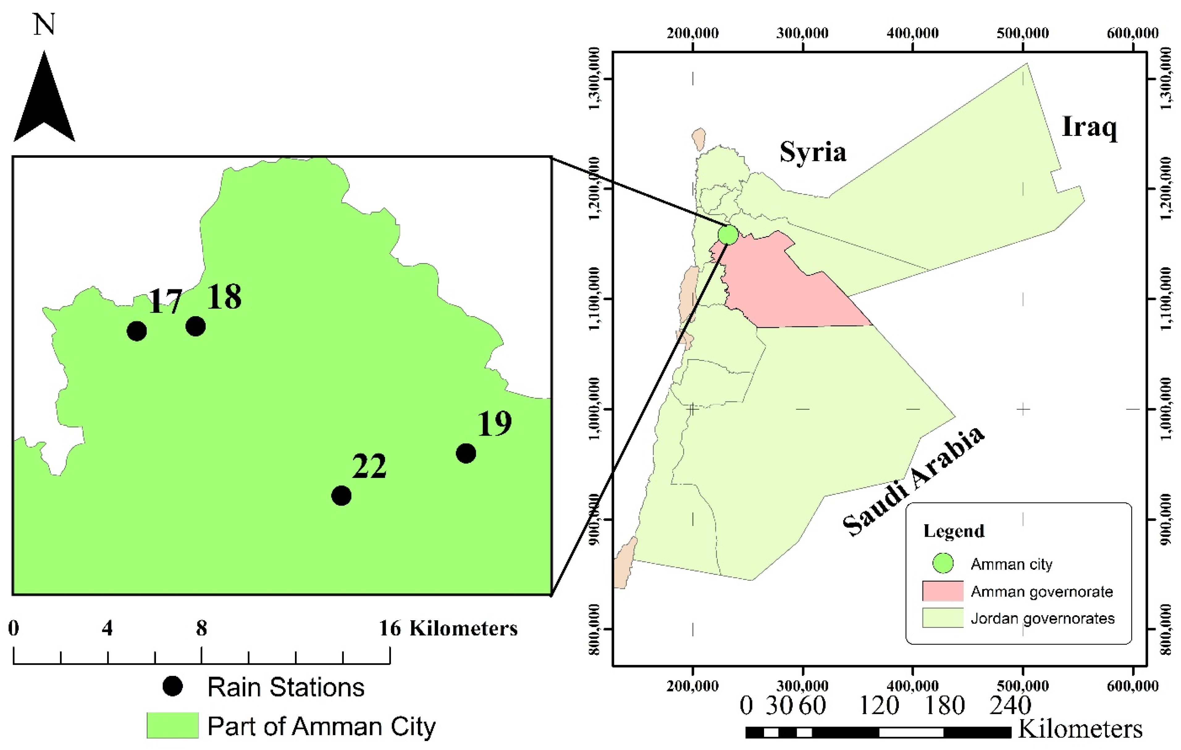
2.1. Study Site and Data Sets

The study site is the city of Amman, Jordan’s capital and economic center. In addition, Amman serves as the political and administrative center of the Jordanian government. Moreover, according to the most recent population data from 2020 [59], it is home to more than 42 percent of Jordan’s total population. Amman has a semiarid climate with hot dry summers and cold, wet winters. The rainy season is between October and May (i.e., the winter season) with an average annual precipitation of 285 mm (mm) [60]. The bulk of this precipitation frequently occurs in January or February, with the maximum precipitation usually occurring in December or January [6].

The city of Amman was chosen for this study due to the recent prevalence of extreme precipitation events [6] and, therefore, there is rising interest from the Jordanian government, greater Amman municipality and various stakeholders for the better analysis of extreme precipitation events to strengthen the city and its inhabitants’ resilience to climate change.

The annual maximum series (AM series) extracted from the daily precipitation data from four weather stations were used in this study. The locations of these stations within the city of Amman are shown in Figure 1, with the station ID, station name, station coordinates, and statistical characteristics of each station given in

Table 1. Selected weather stations’ basic information (i.e., ID, name, coordinates, elevation, data period, and record length) and their statistics based on the annual precipitations.

No.	Station	Station Name	Coordinates a		Elevation	Data	Record Length (years)	Annual Precipitation (mm)
	ID		Latitude	Longitude		Period		Mean	SD	Skewness	Kurt	CV
1	17	SWEILIH	1,159,000	229,500	1000	1942–2016	71	488.85	180.11	0.95	0.89	36.8
2	18	JUBEIHA	1,159,200	232,000	980	1936–2016	79	463.18	165.61	0.38	0.41	35.8
3	19	AMMAN AIRPORT	1,153,800	243,500	790	1937–2016	79	262.55	92.63	0.42	−0.44	35.3
4	22	AMMAN HUSSEIN COLLEGE	1,152,000	238,200	834	1950–2016	66	373.00	137.82	0.65	0.06	36.9

^a Palestine coordinates.

. The daily precipitation records for these four weather stations were collected from the Ministry of Water and Irrigation in Jordan. There were no missing daily precipitation data for the whole period at the selected four stations. Hence, no pretreatment was required for missing data. The POT series (i.e., all daily precipitation whose magnitude exceeded an optimal threshold value) was omitted from this analysis to eliminate the uncertainty associated with determining the appropriate threshold value through various methodologies and their impact on the study results.

2.2. The Modified Mann–Kendall Trend Test

The presence of trends in the AM series was assessed at each station using the nonparametric statistical test of the modified Mann–Kendall (MMK) proposed by Hamed and Rao in 1998 [61]. The Mann–Kendall (MK) test [62,63] is a rank-based test with the benefit of being less sensitive to outliers and missing values as well as not requiring any distribution form for satisfying the data [64]. The latter benefit eliminates the uncertainty associated with meeting the normality assumptions. The MK test includes hypothesis testing, where the null hypothesis, H₀, states that no trend is observed in the data series (i.e., the data are independent, identically distributed, and not correlated). The alternative hypothesis, H_a, states that there will be a monotonic trend in the data series.

The MK test statistics S and Var(S) and standardized test statistics Z for a time series of n observation data points are defined as follows [63]:

$$S={\displaystyle \sum }_{i=1}^{n-1}{\displaystyle \sum }_{j=i+1}^{n}sign\left(x_j-x_i\right)$$

(1)

where x_j − x_i are the sequential data point values at times i and j (x_j is the later-measured value) and sign(x_j− x_i) = {1 if x_j is greater than x_i; 0 if x_j is equal to x_i; and −1 if x_j is less than x_i}.

The statistic S is approximately normally distributed for large values of n [63], with a mean equal to zero, and the variance is given by $Var\left(S\right)=\frac{n\left(n-1\right)\left(2n+5\right)}{18}$. Therefore, the standardized MK test statistic Z is given by:

$$Z=\left\{\begin{array}{c}\frac{S-1}{\sqrt{V\left(S\right)}} \mathrm{for} S>0\\ \\ 0 \mathrm{for} S=0\\ \\ \frac{S+1}{\sqrt{V\left(S\right)}} \mathrm{for} S<0\end{array}\right.$$

(2)

Time series data are often influenced by the presence of autocorrelation, which affects the variance of the Mann–Kendall test (i.e., $Var\left(S\right))$. Thus, the MMK provides variance correction to address this issue according to the following equation:

$$Va{r}^{*}\left(S\right)=Var\left(S\right)\left(\frac{n}{n_e^{*}}\right)=\frac{n\left(n-1\right)\left(2n+5\right)}{18} \left(\frac{n}{n_e^{*}}\right)$$

(3)

where n represents the actual sample size, $n_e^{*}$ is the effective sample size, and $\left(\frac{n}{n_e^{*}}\right)$ is correlation due to the autocorrelation in the data and is given by:

$$\frac{n}{n_e^{*}}=1+\left(\frac{2}{n\left(n-1\right)\left(n-2\right)}\right){\displaystyle \sum }_{i=1}^{n-1}\left(n-1\right)\left(n-i-1\right)\left(n-1-2\right){\rho }_e\left(i\right)$$

(4)

where ${\rho }_e\left(i\right)$ is the autocorrelation function of the ranks of the observations.

The modified MK package within the statistical software S-plus (or R scripting language) was used to obtain the Z statistic value based on the MMK test (https://cran.r-project.org/web/packages/modifiedmk/index.html, accessed date: 18 August 2022).

The Z value can be used to evaluate whether the time series data have a significant trend. A significant trend exists (i.e., the null hypothesis is rejected at a significance level of α) if $\left|Z\right|>Z_{1-\alpha /2}^{}$ in a two-sided test. The $Z_{1-\alpha /2}^{}$ is the critical value and can be obtained from the standard normal table at the significance level α. This critical value is equal to 1.96 at a 5% significance level.

2.3. Extreme Precipitation Probability Distributions

In this research, eight probability distributions (namely, GUM, W3P, GAM, GEV, GP, GLN, PE3, and GLO) were used to fit the AM data series. The cumulative density functions (CDFs) (i.e., F(x) = P(x ≤ x)) of these distributions are shown in

Table 2. The cumulative distribution function (CDF), L-moment estimates of the parameters, and predicted precipitation amount associated with return period T years for the selected extreme probability distribution in this study.

Distributions	CDF	L-Moment Parameters Estimators	Predicted Rainfall Amount Associated with Return Period T Years (Quantiles)
GUM	$F\left(x\right)=e^{-e^{-\left\{\left(x-\xi \right)/\alpha \right\}}}$	$\widehat{\alpha }=\frac{{\lambda }_2}{\ln \left(2\right)}$, $\widehat{\xi }={\lambda }_1-0.5772\widehat{\alpha }$	$X_T= \widehat{\xi }-\widehat{\alpha } \ln \left(-\ln \left[1-\frac{1}{T}\right]\right)$
GAM	$F\left(x\right)=\frac{1}{{\beta }^{\alpha }\mathsf{\Gamma }\left(\alpha \right)}{{\displaystyle \int }}_0^x{x}^{\alpha -1}{e}^{-\frac{x}{\beta }} dx$	If 0 < ${\tau }_2$ < $\frac{1}{2}$ then z = π ${\tau }_2{}^2$, $\widehat{\alpha }\approx \frac{1-0.3080 z}{z-0.05812 z^2+0.01765 z^3}$ If $\frac{1}{2}$ ≤ ${\tau }_2$ < 1 then z = 1 − τ2, $\widehat{\alpha }\approx \frac{0.7213 z-0.5947z^2}{1-2.1817 z+1.2113 z^2}$, $\widehat{\beta }=\frac{{\lambda }_1}{\widehat{\alpha }}$	The quantile of GAM has no explicit analytical form
PE3	$F\left(x\right)=\frac{1}{{\beta }^{\alpha }\mathsf{\Gamma }\left(\alpha \right)}{{\displaystyle \int }}_0^x{\left(x-\xi \right)}^{\alpha -1}{e}^{-\frac{\left(x-\xi \right)}{\beta }} dx$	If 0 < $\left|{\tau }_3\right|$ < $\frac{1}{3}$ then z = 3π ${\tau }_3{}^2$, $\widehat{\alpha }\approx \frac{1+0.2906 z}{z-0.1882 z^2+0.0442 z^3}$ If $\frac{1}{3}$ ≤ $\left|{\tau }_3\right|$ < 1 then z = 1 − $\left|{\tau }_3\right|$, $\widehat{\alpha }\approx \frac{0.36067 z-0.59567z^2+0.25361z^3}{1-2.78861 z+2.5609 z^2-0.77045 z^3}$ $\widehat{\beta }=\frac{\sqrt{\pi }{\lambda }_2\mathsf{\Gamma }\left(\widehat{\alpha }\right)}{\mathsf{\Gamma }\left(\widehat{\alpha }+\raisebox{1ex}{$1$}\!\left/ \!\raisebox{-1ex}{$2$}\right.\right)}$, $\widehat{\xi }={\lambda }_1-\widehat{\alpha }\widehat{\beta }$	The quantile of GAM has no explicit analytical form
W3P	$F\left(x\right)=1-e^{-{\left\{\left(x-\xi \right)/\alpha \right\}}^k}$	First, the shape parameter $\widehat{k}$ is found by iteratively solving equation ${\tau }_3=\frac{1-\frac{3}{2^{1/\widehat{k}}}+\frac{2}{3^{1/\widehat{k}}}}{1-\frac{1}{2^{1/\widehat{k}}}}$, here τ3 is replaced by its sample estimate. $\widehat{\alpha }=\frac{{\lambda }_2}{\mathsf{\Gamma }\left(1+\raisebox{1ex}{$1$}\!\left/ \!\raisebox{-1ex}{$\widehat{k}$}\right.\right)\left(1-\frac{1}{2^{1/\widehat{k}}}\right)}$, $\widehat{\xi }={\lambda }_1-\widehat{\alpha }\mathsf{\Gamma }\left(1+\raisebox{1ex}{$1$}\!\left/ \!\raisebox{-1ex}{$\widehat{k}$}\right.\right)$	$X_T=\widehat{\xi }+\widehat{\alpha } {\left(-\ln \left[\frac{1}{T}\right]\right)}^{\raisebox{1ex}{$1$}\!\left/ \!\raisebox{-1ex}{$\widehat{k}$}\right.}$
GEV	$F\left(x\right)=e^{-e^{-y}}$	$\widehat{k}\approx 7.8590c+2.9554c^2$,$c=\frac{2}{3+{\tau }_3}-\frac{\log 2}{\log 3}$ $\widehat{\alpha }=\frac{{\lambda }_2\widehat{k}}{\left(1-2^{-\widehat{k}}\right)\mathsf{\Gamma }\left(1+\widehat{k}\right)}$, $\widehat{\xi }={\lambda }_1-\alpha \left\{1-\mathsf{\Gamma }\left(1+\widehat{k}\right)\right\}/\widehat{k}$	$X_T=\widehat{\xi }+\frac{\widehat{\alpha }\left\{1-{\left(-\ln \left[1-\frac{1}{T}\right]\right)}^{\widehat{k}}\right\}}{\widehat{k}}$
GP	$F\left(x\right)=1-e^{-y}$	$\widehat{k}=\raisebox{1ex}{$\left(1-3{\tau }_3\right)$}\!\left/ \!\raisebox{-1ex}{$\left(1+{\tau }_3\right)$}\right.$, $\widehat{\alpha }=\left(1+\widehat{k}\right)\left(2+\widehat{k}\right){\lambda }_2$  $\widehat{\xi }={\lambda }_1-\left(2+\widehat{k}\right){\lambda }_2$	$X_T=\widehat{\xi }+\frac{\widehat{\alpha }\left\{1-{\left(1-\left[1-\frac{1}{T}\right]\right)}^{\widehat{k}}\right\}}{\widehat{k}}$
GLO	$F\left(x\right)=\raisebox{1ex}{$1$}\!\left/ \!\raisebox{-1ex}{$\left(1+e^{-y}\right)$}\right.$	$\widehat{k}=-{\tau }_3$, $\widehat{\xi }={\lambda }_1+\frac{\left({\lambda }_2-\widehat{\alpha }\right)}{\widehat{k}}$, $\widehat{\alpha }=\frac{{\lambda }_2}{\mathsf{\Gamma }\left(1+\widehat{k}\right)\mathsf{\Gamma }\left(1-\widehat{k}\right)}$	$X_T=\widehat{\xi }+\frac{\widehat{\alpha }\left\{1-{\left[\left(1-\left[1-\frac{1}{T}\right]\right)/\left[1-\frac{1}{T}\right]\right]}^{\widehat{k}}\right\}}{\widehat{k}}$
GLN	$F\left(x\right)=\varphi \left(y\right)$	$\widehat{k}=-{\tau }_3\frac{2.0466-3.6544{\tau }_3^2+1.8397{\tau }_3^4-0.2036{\tau }_3^6}{1-2.0182{\tau }_3^2+1.242{\tau }_3^4-0.21742{\tau }_3^6}$ $\widehat{\alpha }=\frac{{\lambda }_2\widehat{k}\exp \left(-{\widehat{k}}^2/2\right)}{1-2\varphi \left(-\widehat{k}/\sqrt{2}\right)}$,$\widehat{\xi }={\lambda }_1-\frac{\widehat{\alpha }}{\widehat{k}}\left(1-\exp \left(-{\widehat{k}}^2/2\right)\right)$	The quantile of GLN has no explicit analytical form

$\mathsf{\Gamma }\left( \right)$ is the gamma function, $\varphi \left( \right)$ is the cumulative distribution function of the standard normal distribution, and $y=-k^{-1}ln\left\{1-k\left(x-\xi \right)/\alpha \right\}$.

. In these distributions, the random variable x represents an extreme precipitation amount, ξ is the location parameter, α is the scale parameter, and k is the shape parameter. Additionally, Table 2 provides the quantity of the extreme precipitation (i.e., the quantile) denoted as X_T for each of these eight distributions at a specified return period of T years. The cumulative density function F, or non-exceedance probability, at a particular event x is expressed mathematically in terms of return period T in years as $F=1-\frac{1}{T}$. The $\widehat{\xi }$, $\widehat{\alpha }$, and $\widehat{k}$ are the estimates of ξ, α, and k, respectively. More details on this are given in Section 2.4.

2.4. L-Moment Method for Parameter Estimation

The L-moment method was applied to estimate the distribution parameters in this study due to the fact of its advantages over other estimation methods, as reported earlier in Section 1. It is noteworthy that this work did not attempt to quantify the uncertainty associated with the parameter estimate as a result of varying estimation methods or resulting from the use of various estimation methods. More details on the L-moment method and its advantages can be found in [31,39] and briefly described herein.

L-moments are linear combinations of probability-weighted moments (PWMs), as proposed by Greenwood et al. (1979) [65]. In practice, L-moments are estimated using the observation data x_(i) from a finite sample of size n that have been arranged in ascending order. The first four L-moments are given by ${\lambda }_1=b_0=\overline{X}$, ${\lambda }_2=2b_1-b_0$, ${\lambda }_3=6b_2-6b_1+b_0$, and ${\lambda }_4=20b_3-30b_2+12b_1-b_0$, where b₀, b₁, b₂, and b₃ are sample unbiased estimators of the PWMs and defined by [31]:

$$b_0={\displaystyle \sum }_{i=1}^n\frac{1}{n}{x}_{\left(i\right)}$$

(5)

$$b_1={\displaystyle \sum }_{i=2}^n\frac{\left(i-1\right)}{n\left(n-1\right) } x_{\left(i\right)}$$

(6)

$$b_2={\displaystyle \sum }_{i=3}^n\frac{\left(i-1\right)\left(i-2\right) }{n\left(n-1\right)\left(n-2\right) } x_{\left(i\right)}$$

(7)

$$b_3={\displaystyle \sum }_{i=1}^n\frac{\left(i-1\right)\left(i-2\right)\left(i-3\right)}{n\left(n-1\right)\left(n-2\right)\left(n-3\right) } x_{\left(i\right)}$$

(8)

In addition, Hosking [39] defined other dimensionless quantities called L-moment ratios, which are computed as the L-variation τ₂ (τ₂ = λ₂/λ₁), L-skewness τ₃ (τ₃ = λ₃/λ₂), and L-kurtosis τ₄ (τ₄ = λ₄/λ₂). The estimates of the location ξ, scale α, and shape k parameters (denoted as $\widehat{\xi }$,$\widehat{\alpha }$, and $\widehat{k}$, respectively) of the eight distributions by L-moments are given in Table 2, as developed in [31].

2.5. Kolmogorov–Smirnov (KS) Goodness-of-Fit Test

The Kolmogorov–Smirnov (KS) goodness-of-fit test was used in this study to select the optimal distribution to fit the AM data series for each weather station at a 95% confidence level from aforementioned probability distributions. It is a nonparametric statistical test based on the testing of the hypothesis technique [66,67]. The null hypothesis (H_o) states that the data suitably fit the candidate probability distribution at a specified confidence level. The KS test compares the empirical and theoretical cumulative distribution function. The empirical cumulative distribution F_n(x) obtained from the observed data (i.e., AM data series) is given by Equation (9). The KS test statistic (D_max) is the maximum absolute difference between F₀(x) and F_n(x) over the entire range of X and mathematically expressed as $D_{max}=max\left|F_0\left(x\right)-\left.F_n\left(x\right)\right|\right.$. The null hypothesis (H_o) is rejected if the calculated D_max value exceeds a critical value (D_critical = 1.36/$\sqrt{n}$) for the sample size n and 95% confidence level.

$$F_n\left(x\right)=\left\{\begin{array}{c}0 , x<x_1\\ \frac{k}{n} , x_k<x<x_{k+1}\\ 1 , x>x_n\end{array}\right.$$

(9)

where x₁,x₂,…..,x_n are the values of the ordered extreme precipitation amount; k is the rank of the precipitation amount in the data organized in an ascending order. The probability distribution that best-fit the data among the applicable distributions is the one with the minimum value of the KS test statistic.

2.6. Bootstrap Approach

Resampling using the bootstrap approach was originally introduced in 1979 by Efron [68] to estimate the variance of a sample statistic. This approach was further modified in 1993 by Efron and Tibshirani [69]. It is a nonparametric statistical approach that has the benefit of eliminating assumptions regarding the statistical distribution representing the data sample to process this data (i.e., normality assumption). In addition, this approach has the benefit that it is easier to implement relative to classical resampling approaches. The rationale behind the bootstrap approach is that the sample values are the best indicator of the true distribution, even when information concerning the true distribution is unavailable [70]. The bootstrap approach was used in this study to quantify the uncertainty in terms of the confidence intervals of the predicted extreme precipitation estimates and to evaluate the impact of the data record length on the results of the summary statistics characteristics of the data set (i.e., the average, standard deviation (SD), coefficient of variation (CV), skewness, and kurtosis) and, therefore, the predicted extreme precipitation estimates.

The basic concept of bootstrap was to create several replicate sample series (i.e., bootstrap samples) of size n from the original observed sample of an unknown distribution. This procedure involves randomly selecting data from the original sample with replacements. Then, these bootstrap samples were utilized to perform various statistical tests [68]. Although the bootstrap procedure requires a relatively intensive amount of computing [57], only a minimal amount of programming is necessary. The bootstrap technique was carried out in this study using the S-Plus programming language. The bootstrap procedure used in this study to construct the two-side confidence interval and the sampling distribution of predicted extreme precipitation estimates can be summarized as follows:

(1)

For each selected weather station, 10,000 bootstrap samples of sizes n were extracted from the AM extreme precipitation data series.

(2)

For each bootstrap sample, the extreme precipitation quantile (X_T) at a chosen return period of T years was extracted using the best-fit probability distribution to represent that station using the L-moment method for parameters estimation.

(3)

The 10,000 X_T values for a chosen return period of T years (obtained in step (2)) in ascending order were ranked.

(4)

The two-sided confidence intervals for the ranked X_T at α = 5% (i.e., 95% confidence interval) were obtained. For the 10,000 resampling times used in this study, the upper and lower values of the two-sided confidence interval for X_T correspond to the 9750th (i.e., 97.5th percentile) and 250th (i.e., 2.5th percentile) of the ranked X_T values.

(5)

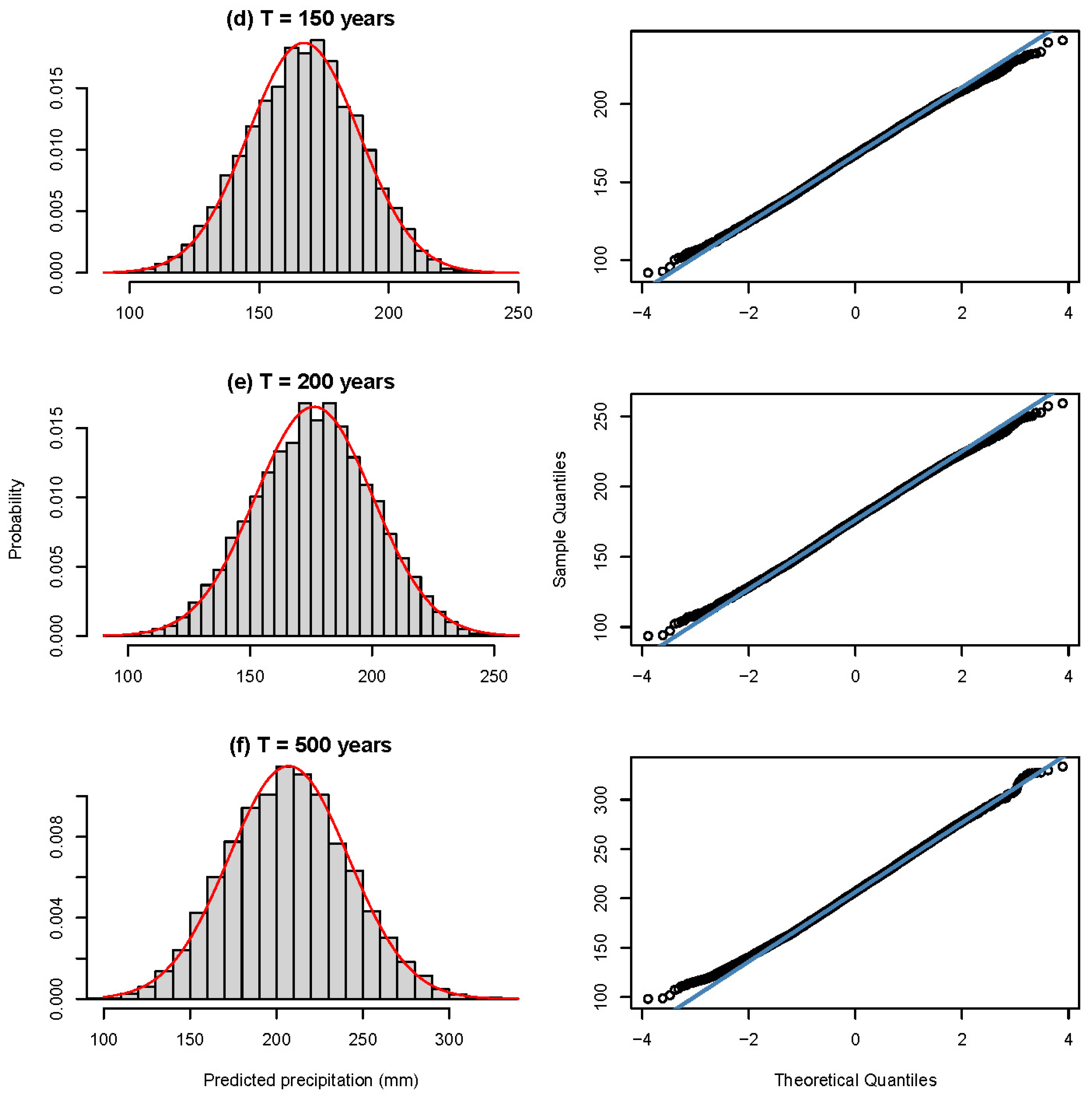
The bootstrap sampling distributions for the extreme precipitation quantile (X_T) from 10,000 X_T values were obtained for a chosen return period of T years (obtained in step (2)).

(6)

The expected value of the sampling distribution of the extreme precipitation quantile (X_T) (obtained in step (5)) was obtained.

(7)

Steps (2) to (6) were repeated for each of the selected weather stations for a different return period of T years.

In addition, to investigate the impact of the data record length on the results of the summary statistics characteristics of the data set, the average, SD, CV, skewness, and kurtosis were calculated for each 10,000 bootstrap sample obtained in step (1) from the above procedure. Then, the average and the standard deviation of the 10,000 average, SD, CV, skewness, and kurtosis were obtained. These two steps were repeated for the different sample sizes n (i.e., n = 10, 15, 20, 30, 40, 50, 75, 80 100,150, 200, and 500 years).

3. Results and Discussion

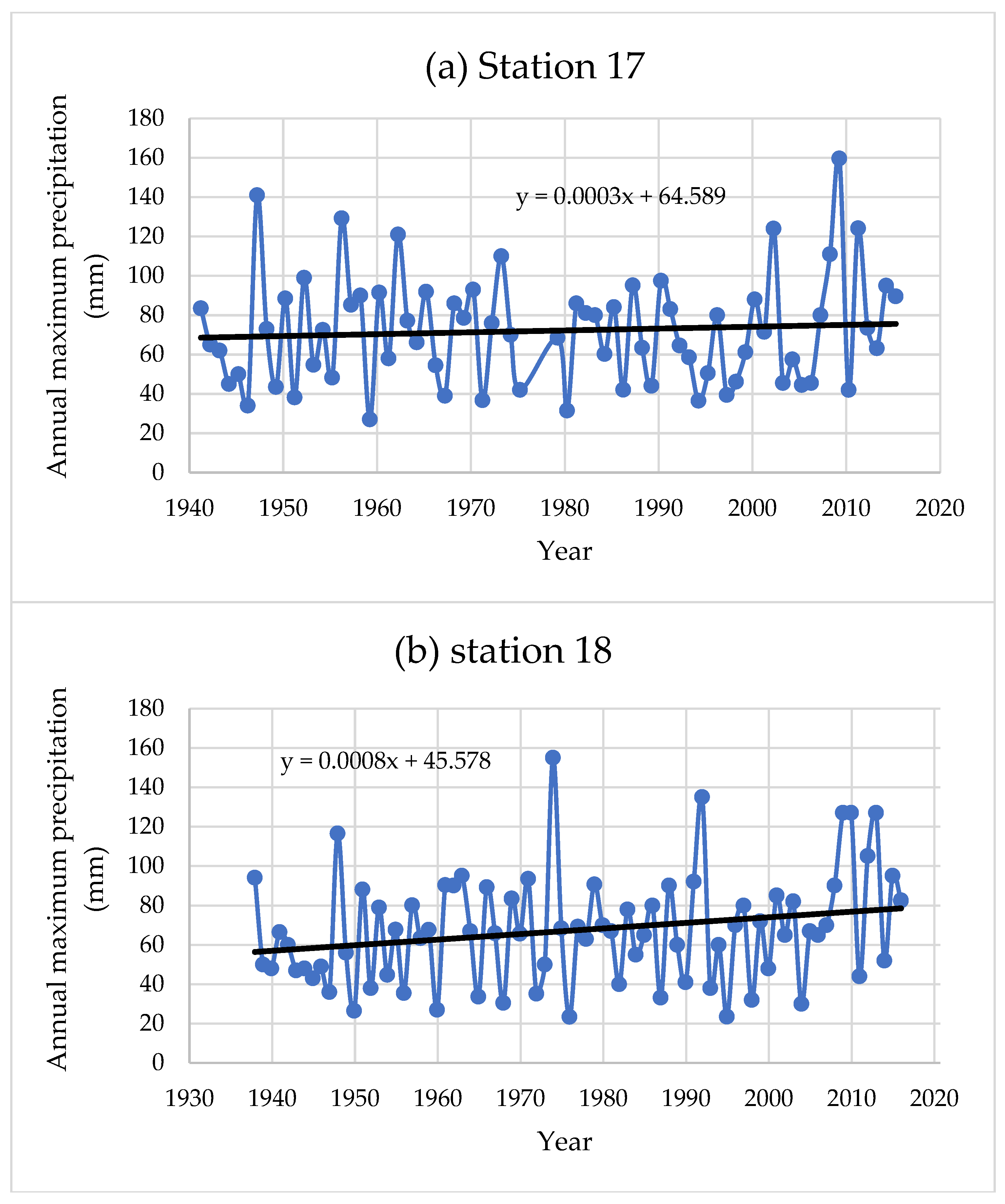
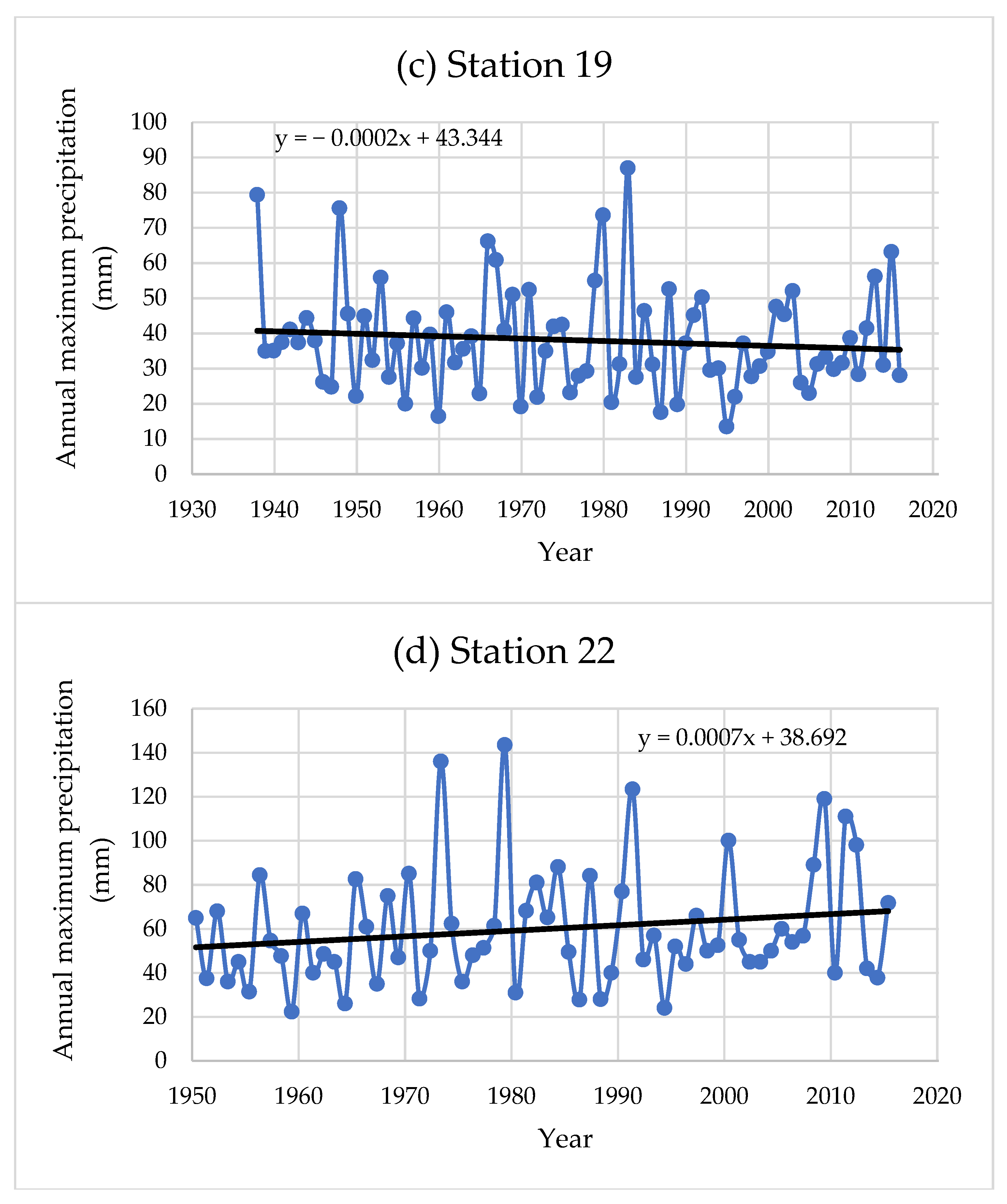
3.1. Trend Analysis of Extreme Precipitation

The AM series is presented in Figure 2 for each selected weather station. In addition,

Table 3. Summary of the modified Mann–Kendall (MMK) trend test statistic value (Z) and the Kolmogorov–Smirnov (KS) goodness-of-fit test statistic value (D_max) of the AM data series for the selected weather stations.

Station	MMK Trend Test	KS Goodness-of-Fit Test Dmax Value
ID	Z Value	GEV	GP	GLO	PE3D	W3P	GLN	GAM	GUM	Best Distribution
17	0.46	0.078	0.083	0.091	0.074	0.064	0.077	0.074	0.082	W3P
18	1.93	0.069	0.101	0.066	0.069	0.074	0.067	0.076	0.090	GLO
19	−0.73	0.044	0.083	0.060	0.052	0.061	0.043	0.060	0.050	GLN
22	1.68	0.043	0.082	0.055	0.062	0.068	0.050	0.077	0.068	GEV

summarizes the results of the modified Mann–Kendall (MMK) test statistic value Z obtained at each station for the AM data series. The Z values indicate that no statistically significant trend was detected in the AM data series (i.e., the null hypothesis H_o for the MMK test was accepted, since $\left|Z^{MK}\right|<1.96$). The above results (Figure 2 and Table 3) indicate that the AM data series was stationary, independent, and identically distributed. Therefore, the frequency analysis stationarity and serial independence presumptions were valid.

3.2. The Best-Fit Probability Distribution for Extreme Precipitation

In this study, eight probability distributions were used to fit the AM extreme precipitation series (i.e., GUM, W3P, GEV, GLN, GLO, GP, GAM, and PE3). The GUM and GAM distributions were two parameters distributions (i.e., location and scale parameters for GUM and shape and scale for GAM). The remaining probability distributions were three parameters distributions (i.e., shape, scale, and location parameter). The parameters for each distribution were estimated by the L-moment method. Table 3 summarizes the results of the KS goodness-of-fit test. The table shows the test statistics value D_max obtained at each station for the AM series using the eight distributions. The smaller the test statistic D_max value, the better the probability distribution fits the extreme precipitation data series. displays the optimal distribution for each station. All distributions passed the KS test at the 5% significance level, indicating that the sample distribution followed the theoretical distribution (i.e., the null hypothesis H_o for the KS test was accepted), since the D_n values were less than the related critical value (D_critica = 1.36/$\sqrt{n}$ for a sample size n at the 5% significance level).

Based on the KS test (Table 3), the AM series best-fit distribution for stations 17, 18, 19, and 22 was the W3P, GLO, GLN, and GEV, respectively. These findings suggest that various distributions may suit the AM series for various stations. As a result, it is emphasized that an uncertainty analysis should be conducted using the best-fit probability distribution for extreme precipitation data series rather than a predefined single probability distribution based on modern extreme value theory. As a result, the best-fit distribution at each station was used for the uncertainty analysis at that station, which is the innovative aspect of this paper. This will reduce the uncertainty in the predicted extreme precipitation value associated with selecting the proper probability distribution for the given extreme data.

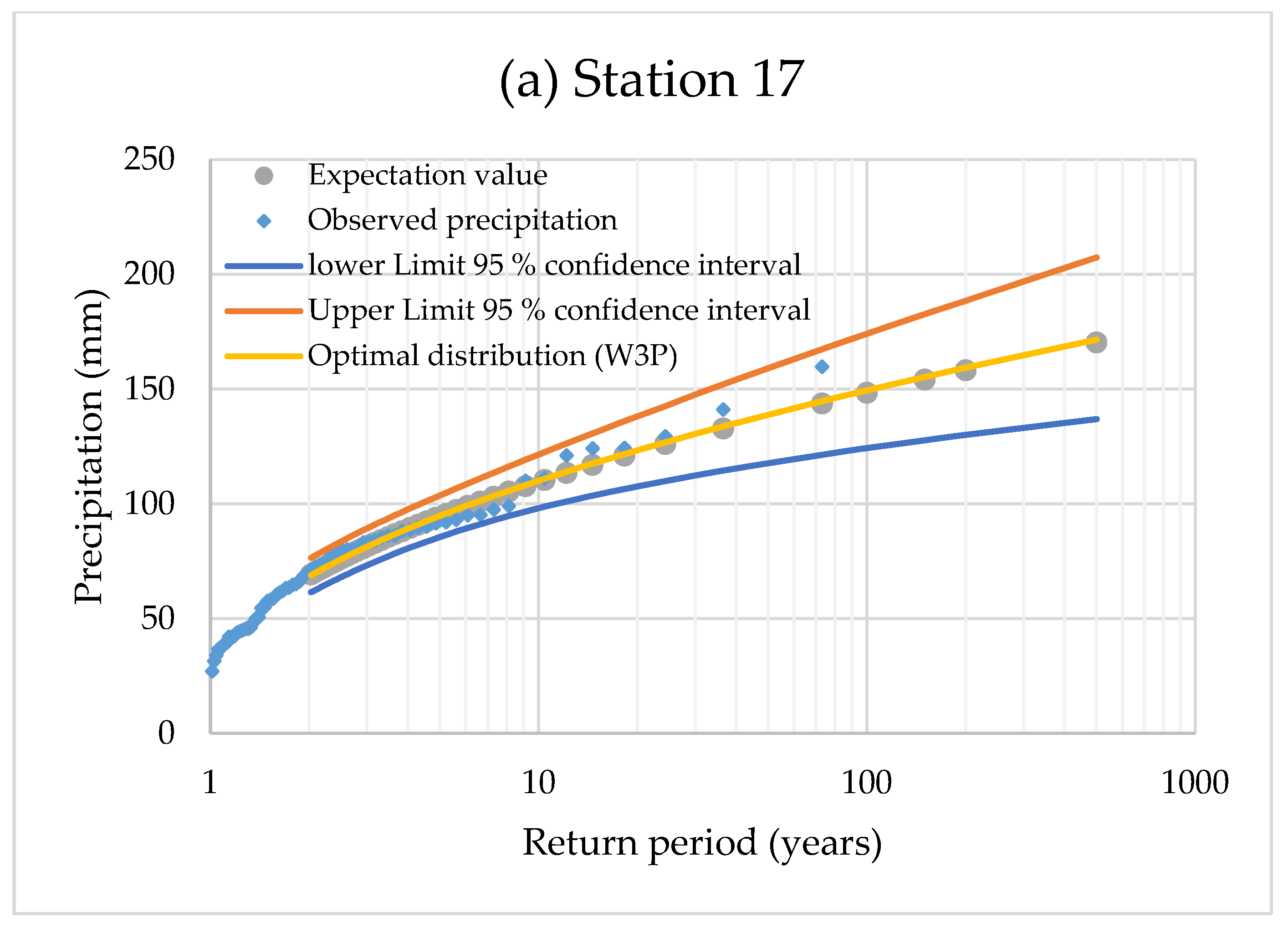
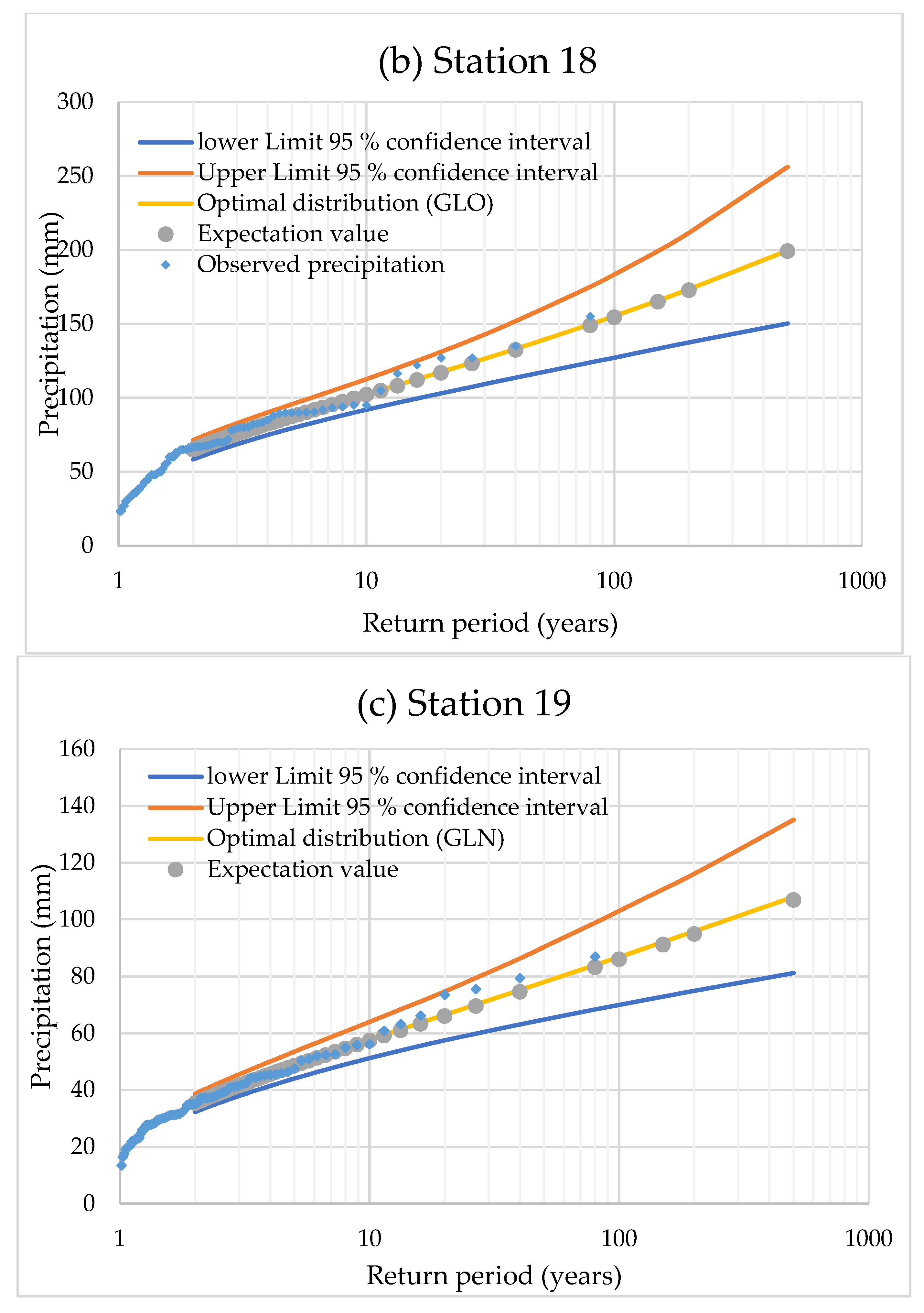
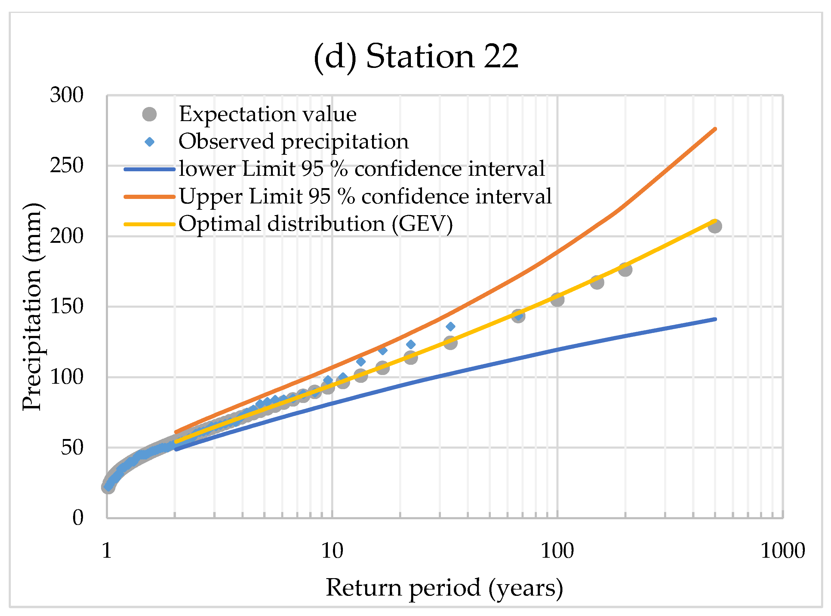
3.3. Quantile Estimations and Uncertainty Bounds

The predicted precipitation quantiles X_T based on the optimal distribution obtained from equations at Table 2 (henceforth named conventional method X_T) as well as their uncertainty bounds (i.e., 95% confidence intervals estimated based on bootstrap resampling) for the selected location at different return periods are presented in Figure 3 along with the observed AM extreme precipitation data and the expected value, which form the sampling distribution. These expected values obtained from the sampling distributions of X_T at a particular return period will represent the predicted extreme precipitation quantile of that return period (henceforth named sampling distribution X_T). The return periods (T) associated with the observed AM precipitation extremes were calculated using the Weibull plotting position formula, $T=\frac{1}{1-\frac{i}{n+1}}$, where i is the rank of the extreme precipitation amount in the data series organized in ascending order, and n is the data series length.

Table 4. Predicted precipitation quantile, their lower and upper 95% confidence limits, the relative differences of the confidence limits from the predicted quantile and expectation value that form the sampling distribution.

Station: 17
Return period, T (years)	2	5	10	20	50	100	150	200	500
Predicted precipitation quantiles (mm)	68.42	94.78	110.10	123.37	138.86	149.47	155.33	159.35	171.53
Upper Limit 95% confidence interval (ULC) (mm)	75.97	103.63	121.48	138.29	159.18	174.12	182.70	188.53	207.42
Lower Limit 95% confidence interval (LLC) (mm)	61.09	85.54	98.10	107.65	117.87	124.30	127.70	130.10	136.89
ULC relative differences from the predicted (%)	11.04	9.34	10.33	12.09	14.63	16.50	17.62	18.31	20.92
LLC relative differences from the predicted (%)	−10.70	−9.75	−10.90	−12.74	−15.11	−16.84	−17.78	−18.36	−20.20
Expectation value (mm)	68.59	94.42	109.45	122.49	137.75	148.24	154.04	158.03	170.13
Station: 18
Return period, T (years)	2	5	10	20	50	100	150	200	500
Predicted precipitation quantiles (mm)	64.76	87.47	102.43	117.44	138.31	155.25	165.72	173.41	199.52
Upper Limit 95% confidence interval (ULC) (mm)	71.42	95.61	112.68	131.10	159.04	183.39	199.23	211.64	256.16
Lower Limit 95% confidence interval (LLC) (mm)	58.37	79.46	91.97	102.98	116.95	127.13	133.24	137.47	150.21
ULC relative differences from the predicted (%)	10.28	9.31	10.00	11.64	14.99	18.13	20.22	22.04	28.38
LLC relative differences from the predicted (%)	−9.87	−9.15	−10.21	−12.31	−15.44	−18.12	−19.60	−20.73	−24.71
Expectation value (mm)	64.87	87.25	102.01	116.84	137.55	154.46	164.96	172.69	199.13
Station: 19
Return period, T (years)	2	5	10	20	50	100	150	200	500
Predicted precipitation quantiles (mm)	35.26	48.70	57.75	66.53	78.06	86.88	92.10	95.83	107.96
Upper Limit 95% confidence interval (ULC) (mm)	38.71	53.57	64.07	74.75	90.26	103.03	110.66	116.08	135.13
Lower Limit 95% confidence interval (LLC) (mm)	32.31	44.11	51.28	57.54	64.82	70.03	72.94	74.98	81.24
ULC relative differences from the predicted (%)	9.80	10.00	10.95	12.36	15.62	18.59	20.16	21.13	25.16
LLC relative differences from the predicted (%)	−8.35	−9.41	−11.19	−13.50	−16.97	−19.39	−20.80	−21.76	−24.75
Expectation value (mm)	35.39	48.60	57.46	66.06	77.37	86.03	91.17	94.86	106.85
Station: 22
Return period, T (years)	2	5	10	20	50	100	150	200	500
Predicted precipitation quantiles (mm)	53.88	77.31	94.43	112.16	137.19	157.61	170.23	179.50	210.93
Upper Limit 95% confidence interval (ULC) (mm)	60.64	87.29	106.97	127.85	160.07	188.80	207.88	222.39	276.12
Lower Limit 95% confidence interval (LLC) (mm)	48.35	67.93	81.42	93.98	108.88	119.51	125.28	129.22	141.12
ULC relative differences from the predicted (%)	12.56	12.91	13.28	13.99	16.68	19.79	22.12	23.89	30.91
LLC relative differences from the predicted (%)	−10.26	−12.13	−13.77	−16.21	−20.63	−24.18	−26.41	−28.01	−33.10
Expectation value (mm)	54.12	77.13	93.78	110.96	135.16	154.95	167.20	176.24	207.04

illustrates the relative differences of the lower and upper 95% confidence limits from the predicted quantile.

The findings revealed that the precipitation quantiles were subject to significant uncertainty. Furthermore, the band of uncertainty intervals increased as the return period rose (Figure 3). This suggests that, among the return periods taken into account in this study, the predicted precipitation quantiles for the 500- year return period had the largest level of uncertainty (especially for station 22). For weather station 22, for example, the relative differences (%) of the lower and upper 95% confidence limits from the predicted quantile ranged from −10.26 to 12.56 for the return periods of the 2 years and increased with the increase in the return periods to range from −33.10 to 30. 91 for a return period of 500 years. These confidence intervals for several return periods are beneficial for water sector policymakers to take appropriate actions, such as the design of various water infrastructures (construction of a proper drainage system, construction of flood control structures, etc.) to control and minimize the risks of large damages caused by the frequent precipitation extremes that have occurred in recent years in Amman. Another noteworthy finding from Figure 3 is that the values of the observed precipitation were within the confidence interval limits.

Figure 4 depicts a histogram as well as a normal quantile plot of the bootstrap sampling distribution of extreme precipitation quantile (X_T) for station 22 (as example). These plots indicate the sampling distribution of X_T for the different return periods (i.e., different non exceedance probability). In a similar way, it was possible to obtain the sampling distributions of X_T at any return period. For other locations, the findings are comparable to those displayed in Figure 4 and, as a consequence, they are not provided in this article as a separate figure. The findings from other locations are provided in Figures S1–S3 for the weather stations 17, 18, and 19, respectively, in the Supplementary Materials. This article utilized the normal quantile plot to determine if the sampling distribution of X_T matched with a normal distribution.

As can be seen in Figure 4, the normal distribution may match well with the probability histograms. In addition, the normal quantile plot shows that the fitted normal frequency line was consistent with the observed data. Therefore, the sampling distribution of the extreme precipitation quantile was approximately the normal distribution, even if the population were not normal (based on the central limit theorem; when the sample size is large enough, the sample size is 10,000). Accordingly, the expected value of the bootstrap sampling distribution of the extreme precipitation quantile (X_T) was evaluated (i.e., the mean of sampling distribution) at a particular return period and are shown in Table 4.

As seen in in Table 4, the results of the extreme precipitation quantile (X_T) obtained by the two methods (the conventional and the sampling distribution methods) look quite similar. Nevertheless, compared to the conventional method, the sampling distribution method provides more information regarding the statistical parameter of interest (i.e., X_T). The bootstrap sampling distribution is useful for quantifying the behavior of a parameter estimate (i.e., how the statistic varies across many random data sets, such as its standard error, skewness, bias, or for calculating confidence intervals). Consequently, the estimation of X_T at a particular non exceedance probability (i.e., particular return period) should be based on its sampling distribution. Since, for a given data set, this sampling distribution allows not only the point estimation of the precipitation quantile as the expected value of sampling distribution (i.e., sampling distribution X_T), which can be employed in place of the X_T based on the optimal distribution obtained by conventional method (i.e., conventional method X_T), but also quantifying the uncertainty associated with X_T in terms of the confidence interval.

3.4. Effects of Data Resolution from which the AMS Was Extracted

A simulation using the bootstrap method was carried out to address the research question of how the record length of the data set alters the results of its summary statistics characteristics (i.e., the average, SD, CV, skewness, and kurtosis). The SD value of each characteristic of these summary statistics was used to quantify their variability over different record lengths. These characteristics may influence the effectiveness of the probability distributions to accurately depict the precipitation extremes at the investigated weather stations [6,11] and, consequently, affects their projected precipitation quantile estimate. The 10,000 bootstrap resampling summary statistics characteristics results and their variability in terms of their standard deviation are summarized in

Table 5. The results of the 10,000 bootstrap samples summary statistics characteristics (i.e., the average, standard deviation (SD), coefficient of variation (CV), skewness, and kurtosis) and their standard deviation for the different record lengths for station 18.

Record Length	Average		Standard Deviation (SD)		Coefficient of Variation (CV)		Skewness		Kurtosis
	Average	SD	Average	SD	Average	SD	Average	SD	Average	SD
10	67.692	8.852	26.711	7.014	0.395	0.093	0.334	0.599	2.548	1.028
15	67.653	7.199	27.030	5.727	0.400	0.076	0.440	0.545	2.818	1.024
20	67.576	6.173	27.170	4.939	0.402	0.066	0.498	0.485	2.964	1.021
30	67.570	5.047	27.345	3.994	0.405	0.053	0.571	0.398	3.151	0.953
40	67.556	4.356	27.384	3.452	0.406	0.046	0.603	0.340	3.232	0.853
50	67.531	3.888	27.457	3.102	0.407	0.041	0.626	0.303	3.287	0.770
75	67.555	3.186	27.539	2.507	0.408	0.033	0.652	0.239	3.350	0.618
80	67.555	3.109	27.540	2.437	0.408	0.032	0.655	0.234	3.356	0.605
90	67.549	2.910	27.553	2.277	0.408	0.030	0.661	0.217	3.370	0.565
100	67.542	2.745	27.554	2.183	0.408	0.029	0.664	0.208	3.376	0.534
150	67.536	2.237	27.557	1.782	0.408	0.024	0.674	0.167	3.407	0.436
200	67.540	1.943	27.565	1.531	0.408	0.021	0.680	0.143	3.420	0.375
500	67.520	1.229	27.589	0.972	0.409	0.013	0.689	0.090	3.439	0.234
Max.	67.692	8.852	27.589	7.014	0.409	0.093	0.689	0.599	3.439	1.028
Min.	67.520	1.229	26.711	0.972	0.395	0.013	0.334	0.090	2.548	0.234
Percent change	0.255	620.312	3.288	621.234	3.348	613.520	106.179	569.526	34.982	338.975

Observed data summary statistics characteristics for station 18 are as follows: average = 67.52, SD = 27.759, CV = 0.411, skewness = 0.695, and kurtosis = 3.455.

for the different record lengths for station 18, as an example. The findings of the other locations are provided in Tables S1–S3 for weather stations 17, 19, and 22, respectively, in the Supplementary Materials.

As anticipated, the findings in Table 5 clearly demonstrated that the larger the record length, the less the variability in terms of the SD of the average, SD, CV, skewness, and kurtosis of 10,000 bootstrap samples. The SD values of the 10,000 bootstrap samples average values varied from 8.852 (when n = 10 years) to 1.229 (when n = 500 years), which presents a 620.312% change. The SD values of the 10,000 bootstrap samples SD values were in the range of 7.014 (n = 10 years)–0.972 (n = 500 years), which presents a 621.234% change. The SD values of the 10,000 bootstrap samples skewness values were between 0.599 (n = 10 years) and 0.090 (n = 500 years), which presents 569.526% change. The SD values of the 10,000 bootstrap samples kurtosis values are in the range from 1.028 (when n = 10 years) to 0.234 (when n = 500 years) which presents 338.975% change.

Another noteworthy finding from Table 5 is that the average values of the 10,000 bootstrap samples average and SD values were almost the same as the observed data average and SD values (79 years record length) with percent change of 0.255% and 3.288%, respectively. While the average values of the 10,000 bootstrap samples skewness and kurtosis values were different from the observed data skewness and kurtosis values, particularly when the record length was small, with percent change of 106.179% and 34.982%, respectively. This suggests that a longer record length is desirable to decrease sampling uncertainty and therefore decrease the error in predicted quantile values. Since the predicted quantile values are highly influenced by these summary statistics characteristics (specially the skewness and kurtosis values) as mentioned earlier.

To further assess the influence of the data record length for station 18, the actual data set was partitioned into subsets representing 12.5%, 25%, and 50% of the original data set length (full original data length n = 79 years). The 50% partition contained two data length scenarios of 39 and 40 years. The 25% partition consisted of four data length scenarios of 19, 20, 20, and 20 years. The 12.5% partition contained eight data length scenarios: one with a duration of nine years and seven with a duration of ten years.

Table 6. Percent change in the probability distribution parameters estimates and precipitation quantile estimates for the various record lengths (segmentation of observed data set lengths were n = 9, 10, 19, 20, 20, 20, 39, and 40 years) for station 18 compared to the full observed data length (full observed data length n = 79 years). The optimal distribution for station 18 was GLO distribution.

Partition Scenarios	Record Length	GLO Probability Distribution Parameters			Return Periods (T)
		Location Parameter (ξ)	Scale Parameter (α)	Shape Parameter (k)	2	5	10	20	50	100	150	200	500
12.5%	9	54.168	14.398	−268.665	54.168	38.435	28.112	18.635	7.088	0.992	5.470	8.539	17.726
	10	24.552	58.928	−281.295	24.552	30.783	30.460	27.766	20.898	13.027	7.221	2.509	16.234
	10	7.421	7.463	−10.147	7.421	3.337	1.445	0.090	1.828	3.007	3.658	4.106	5.470
	10	13.754	18.146	−301.727	13.754	1.194	6.945	14.338	23.242	29.403	32.793	35.106	41.979
	10	8.452	28.300	−118.273	8.452	4.330	12.725	21.175	33.010	42.706	48.733	53.185	68.424
	10	2.341	33.279	−213.760	2.341	9.483	16.282	22.293	29.475	34.461	37.221	39.114	44.794
	10	0.582	21.118	−13.651	0.582	6.247	8.899	11.064	13.537	15.226	16.164	16.811	18.793
	10	0.710	33.018	−289.330	0.710	11.423	18.793	25.360	33.177	38.550	41.498	43.506	49.468
25%	19	16.297	13.858	−41.706	16.297	14.730	13.299	11.765	9.605	7.889	6.857	6.114	3.698
	20	16.952	23.512	−120.323	16.952	16.687	14.709	11.904	7.103	2.670	0.247	2.463	10.363
	20	2.219	11.070	−35.018	2.219	3.749	3.744	3.353	2.465	1.591	1.016	0.584	0.911
	20	0.468	6.807	−41.162	0.468	2.175	3.905	5.574	7.761	9.421	10.395	11.088	13.303
50%	39	7.247	2.603	−19.858	7.247	5.636	4.622	3.654	2.390	1.430	0.865	0.462	0.830
	40	7.209	3.516	−24.548	7.209	5.769	4.746	3.709	2.283	1.151	0.466	0.031	1.670

demonstrates the percent change in the GLO distribution parameters estimates and precipitation quantile estimates when the record lengths were n = 10, 20, 20, 20, 19, 39, and 40 years for station 18 compared to the full observed data length. The GLO distribution was the optimal distribution at this particular station (recall the results of the KS test, Table 3).

As can be seen in Table 6, the GLO distribution parameters estimates were affected by the data record length. For example, the percent change in the shape parameter (k) varied from −10.147 to −301.727 for the 12.5% partition scenario, from −35.018 to −120.323 for the 25% partition scenario, and from −19.858 to −24.548. In addition, it can be seen from Table 6 that the precipitation quantile estimates were greatly affected by the data record length, especially at the higher return periods. For example, the percent change in the precipitation quantile when the return period was 500 years varied from 5.47 to 68.424 for the 12.5% partition scenario, from 0.911 to 13.303 for the 25% partition scenario, and from 0.83 to 1.68. The results in Table 6 also suggest that a series of at least 40 years of data records is needed to obtain reasonably accurate estimates of the precipitation quantiles for 100 year return periods and higher. As is well known, the precipitation quantiles for 100 year return periods and higher are commonly employed in the design of a variety of water-related infrastructure projects. Consequently, the high degree of estimate variability of these quantiles due to the variable length of the data records is a key factor to consider.

4. Conclusions

This research aimed to evaluate the uncertainties in terms of confidence intervals related to the predicted extreme precipitation estimates based on the bootstrap resample simulation framework. In addition, this article studied the impact of the data record length on the predicted extreme precipitation estimates and on the results of summary statistics characteristics of the data set.

The current study was limited to the uncertainty in the statistical modeling of the precipitation extremes associated with the extreme data series (i.e., sampling uncertainty). Future studies should appropriately investigate other sources of uncertainty, such as the model uncertainty (i.e., probability distribution selection) and the parameter uncertainty, (i.e., the uncertainty of parameter estimation), which are not considered in this work.

Based on the results, the following specific conclusions can be drawn:

• The trend analysis indicated that the observed AM series could be considered stationary, independent, and identically distributed. Therefore, the stationarity and serial independence stationarity assumptions were valid for the frequency analysis;
• Different types of probability distributions fit the extreme precipitation data series of the various weather stations, indicating that a careful selection of distributions is essential. Therefore, it is emphasized that an uncertainty analysis should be conducted using the best-fit probability distribution for extreme precipitation data series rather than a predefined single probability distribution for all stations based on modern extreme value theory;
• The sampling distribution of the precipitation quantile at a particular nonexceedance probability (i.e., particular return period) was obtained using a bootstrap resample simulation framework. This bootstrap sampling distribution allowed not only for the point estimation of the precipitation quantile as the expected value of the sampling distribution (i.e., sampling distribution precipitation quantile estimates) but also for quantifying the behavior of the precipitation quantile, such as the confidence interval, standard error, and skewness;
• The uncertainty associated with the used data (i.e., the sampling uncertainty) in a precipitation frequency analysis was evaluated in terms of the 95% confidence intervals based on the bootstrap resample simulation framework. It is concluded that the precipitation quantiles were subject to significant uncertainty and the band of uncertainty intervals increased as the return period increased. These confidence intervals for several return periods are beneficial for water sector policymakers to take appropriate actions to design and manage various water-related infrastructure;
• The extreme precipitation quantile (X_T) obtained by the two methods (the conventional method, typically employed in the literature, and the sampling distribution methods) was comparable;
• The bootstrap resampling for the evaluation of how the record length of the data set alters the results of its summary statistics characteristics showed that a longer record length is desirable to decrease the sampling uncertainty and, therefore, decrease the error in the predicted quantile values, since the predicted quantile values are highly influenced by these summary statistics characteristics (specially the skewness and kurtosis values).
• The study showed that the distribution parameters estimates as well as the precipitation quantile estimates (specially at the higher return periods) were greatly affected by the data record length;
• The results suggest that a series of at least 40 years data records is needed to obtain reasonably accurate estimates of the precipitation quantiles for 100 year return periods and higher. Using only 20 to 25 years of data to obtain reasonably accurate estimates of the higher return periods quantile is risky, since it creates high sampling variability relative to the full data length.

In terms of the application, the methodology followed in this study to quantify uncertainty bounds needs to be integrated into any frequency analysis using historical data and, therefore, is expected to contribute to accurately forecasting extreme precipitation quantiles and, thus, will provide the theoretical support to water managers and policymakers for proper actions to design and manage various water-related infrastructures.

References

1. Beskow, S.; Caldeira, T.L.; Rogério, C.; Mello, D.; Faria, L.C.; Alexandre, H.; Guedes, S. Multiparameter probability distributions for heavy rainfall modeling in extreme southern Brazil. J. Hydrol. Reg. Stud. 2015, 4, 123–133. [Google Scholar] [CrossRef] [Green Version]
2. Gocic, M.; Velimirovic, L.; Stankovic, M.; Trajkovic, S. Determining the best fitting distribution of annual precipitation data in Serbia using L-moments method. Earth Sci. Inform. 2020, 14, 633–644. [Google Scholar] [CrossRef]
3. Zhang, Q.; Zhang, J.; Yan, D.; Wang, Y. Extreme precipitation events identified using detrended fluctuation analysis (DFA) in Anhui, China. Theor. Appl. Climatol. 2014, 117, 169–174. [Google Scholar] [CrossRef]
4. Ahmad, I.; Tang, D.; Wang, T.; Wang, M.; Wagan, B. Precipitation Trends over Time Using Mann-Kendall and Spearman’s rho Tests in Swat River Basin, Pakistan. Adv. Meteorol. 2015, 2015, 431860. [Google Scholar] [CrossRef] [Green Version]
5. Zin, W.Z.W.; Jemain, A.A. Statistical distributions of extreme dry spell in Peninsular Malaysia. Theor. Appl. Climatol. 2010, 102, 253–264. [Google Scholar] [CrossRef]
6. Ibrahim, M.N. Generalized distributions for modeling precipitation extremes based on the L moment approach for the Amman Zara Basin, Jordan. Theor. Appl. Climatol. 2019, 138, 1075–1093. [Google Scholar] [CrossRef]
7. Jahanbaksh Asl, S.; Khorshiddoust, A.M.; Dinpashoh, Y.; Sarafrouzeh, F. Frequency analysis of climate extreme events in Zanjan, Iran. Stoch. Environ. Res. Risk Assess. 2013, 27, 1637–1650. [Google Scholar] [CrossRef]
8. Koutsoyiannis, D.; Kozonis, D.; Manetas, A. A mathematical framework for studying rainfall intensity-duration-frequency relationships Demetris. J. Hydrol. 1998, 206, 118–135. [Google Scholar] [CrossRef]
9. Tfwala, C.M.; van Rensburg, L.D.; Schall, R.; Mosia, S.M.; Dlamini, P. Precipitation intensity-duration-frequency curves and their uncertainties for Ghaap plateau. Clim. Risk Manag. 2017, 16, 1–9. [Google Scholar] [CrossRef]
10. Bartolini, G.; Morabito, M.; Crisci, A.; Grifoni, D.; Torrigiani, T.; Petralli, M.; Maracchi, G.; Orlandini, S. Recent trends in Tuscany (Italy) summer temperature and indices of extremes. Int. J. Climatol. 2008, 28, 1751–1760. [Google Scholar] [CrossRef]
11. Ibrahim, M.N. Four-parameter kappa distribution for modeling precipitation extremes: A practical simplified method for parameter estimation in light of the L-moment. Theor. Appl. Climatol. 2022, 150, 567–591. [Google Scholar] [CrossRef]
12. REUTERS. Jordan Flash Floods Kill 21 People, Many of Them School Children on Bus. Available online: https://www.reuters.com/article/us-jordan-floods-idUSKCN1MZ2GI (accessed on 9 August 2022).
13. Roya News. Jordanians Remember Victims of Dead Sea Tragedy. Available online: https://en.royanews.tv/news/23012/2020-10-25 (accessed on 9 August 2022).
14. Chow, V.T.; Maidment, D.R.; Mays, L.W. Applied Hydrology; McGraw-Hill: New York, NY, USA, 1988. [Google Scholar]
15. Singh, V.P. Frequency Distribution. In Handbook of Applied Hydrology; McGraw-Hill Education: New York, NY, USA, 2017. [Google Scholar]
16. Oztekin, T. Wakeby distribution for representing annual extreme and partial duration rainfall series. Meteorol. Appl. 2007, 387, 381–387. [Google Scholar] [CrossRef]
17. Hinge, G.; Hamouda, M.A.; Long, D.; Mohamed, M.M. Hydrologic utility of satellite precipitation products in flood prediction: A meta-data analysis and lessons learnt. J. Hydrol. 2022, 612, 128103. [Google Scholar] [CrossRef]
18. Abebe, W.F.; Ayalew, M.S.; Berhanu, K.B. Detecting Hydrological Variability in Precipitation Extremes: Application of Reanalysis Climate Product in Data-Scarce Wabi Shebele Basin of Ethiopia. J. Hydrol. Eng. 2022, 27, 5021035. [Google Scholar] [CrossRef]
19. Hinge, G.; Mazumdar, M.; Deb, S.; Kalita, M.K. District-level assessment of changes in extreme rainfall indices in Barak and other basins in Indian Himalayan states: Risks and opportunities. Model. Earth Syst. Environ. 2022, 8, 1145–1155. [Google Scholar] [CrossRef]
20. Ouali, D.; Cannon, A.J. Estimation of rainfall intensity–duration–frequency curves at ungauged locations using quantile regression methods. Stoch. Environ. Res. Risk Assess. 2018, 32, 2821–2836. [Google Scholar] [CrossRef] [Green Version]
21. Lettenmaier, D.P.; Potter, K.W. Testing Flood Frequency Estimation Methods Using a Regional Flood Generation Model. Water Resour. Res. 1985, 21, 1903–1914. [Google Scholar] [CrossRef]
22. Hosking, J.R.M.; Wallis, J.R.; Wood, E.F. An appraisal of the regional flood frequency procedure in the UK Flood Studies Report. Hydrol. Sci. J. 1985, 30, 85–109. [Google Scholar] [CrossRef] [Green Version]
23. Lettenmaier, D.P.; Wallis, J.R.; Wood, E.F. Effect of regional heterogeneity on flood frequency estimation. Water Resour. Res. 1987, 23, 313–323. [Google Scholar] [CrossRef] [Green Version]
24. Du, H.; Xia, J.; Zeng, S.; She, D.; Liu, J. Variations and statistical probability characteristic analysis of extreme precipitation events under climate change in Haihe River Basin, China. Hydrol. Process. 2014, 28, 913–925. [Google Scholar] [CrossRef]
25. Yilmaz, A.G.; Perera, B.J.C. Extreme Rainfall Nonstationarity Investigation and Intensity–Frequency–Duration Relationship. J. Hydrol. Eng. 2014, 19, 1160–1172. [Google Scholar] [CrossRef] [Green Version]
26. Yang, T.; Xu, C.-Y.; Shao, Q.-X.; Chen, X. Regional flood frequency and spatial patterns analysis in the Pearl River Delta region using L-moments approach. Stoch Env. Res Risk Assess 2010, 24, 165–182. [Google Scholar] [CrossRef]
27. Sen Roy, S.; Balling Jr, R.C. Trends in extreme daily precipitation indices in India. Int. J. Climatol. 2004, 24, 457–466. [Google Scholar] [CrossRef]
28. Liu, B.; Chen, X.; Chen, J.; Chen, X. Impacts of different threshold definition methods on analyzing temporal-spatial features of extreme precipitation in the Pearl River Basin. Stoch. Environ. Res. Risk Assess. 2017, 31, 1241–1252. [Google Scholar] [CrossRef]
29. Liu, B.; Chen, J.; Chen, X.; Lian, Y.; Wu, L. Uncertainty in determining extreme precipitation thresholds. J. Hydrol. 2013, 503, 233–245. [Google Scholar] [CrossRef]
30. Xia, J.; She, D.; Zhang, Y.; Du, H. Spatio-temporal trend and statistical distribution of extreme precipitation events in Huaihe River Basin during 1960–2009. J. Geogr. Sci. 2012, 22, 195–208. [Google Scholar] [CrossRef]
31. Hosking, J.R.M.; Wallis, J.R. Regional Frequency Analysis: An Approach Based on L-Moments; Cambridge University Press: Cambridge, UK, 1997. [Google Scholar]
32. Coles, S. An Introduction to Statistical Modeling of Extreme Values; Springer: London, UK, 2001. [Google Scholar]
33. Abolverdi, J.; Khalili, D. Development of Regional Rainfall Annual Maxima for Southwestern Iran by L-Moments. Water Resour. Manag. 2010, 24, 2501–2526. [Google Scholar] [CrossRef]
34. Deni, S.M.; Suhaila, J.; Wan Zin, W.Z.; Jemain, A.A. Spatial trends of dry spells over Peninsular Malaysia during monsoon seasons. Theor. Appl. Climatol. 2010, 99, 357–371. [Google Scholar] [CrossRef]
35. She, D.; Xia, J.; Song, J.; Du, H. Spatio-temporal variation and statistical characteristic of extreme dry spell in Yellow River Basin, China. Theor. Appl. Clim. 2013, 112, 201–213. [Google Scholar] [CrossRef]
36. Zakaria, Z.A.; Shabri, A.; Ahmad, U.N. Regional Frequency Analysis of Extreme Rainfalls in the West Coast of Peninsular Malaysia using Partial L-Moments. Water Resour. Manag. 2012, 26, 4417–4433. [Google Scholar] [CrossRef]
37. Saf, B. Regional Flood Frequency Analysis Using L-Moments for the West Mediterranean Region of Turkey. Water Resour. Manag. 2009, 23, 531–551. [Google Scholar] [CrossRef]
38. Adamowski, K. Regional analysis of annual maximum and partial duration flood data by nonparametric and L-moment methods. J. Hydrol. 2000, 229, 219–231. [Google Scholar] [CrossRef]
39. Hosking, J.R.M. L-Moments: Analysis and Estimation of Distributions Using Linear Combinations of Order Statistics. J. R. Stat. Soc. B 1990, 52, 105–124. [Google Scholar] [CrossRef]
40. Pandey, M.D.; Van Gelder, P.H.A.J.M.; Vrijling, J.K. The estimation of extreme quantiles of wind velocity using L-moments in the peaks-over-threshold approach. Struct. Saf. 2001, 23, 179–192. [Google Scholar] [CrossRef]
41. Asquith, W.H. L-moments and TL-moments of the generalized lambda distribution. Comput. Stat. Data Anal. 2007, 51, 4484–4496. [Google Scholar] [CrossRef]
42. Vogel, R.M.; Fennessey, N.M. L moment diagrams should replace product moment diagrams. Water Resour. Res. 1993, 29, 1745–1752. [Google Scholar] [CrossRef]
43. Sankarasubramanian, A.; Srinivasan, K. Investigation and comparison of sampling properties of L-moments and conventional moments. J. Hydrol. 1999, 218, 13–34. [Google Scholar] [CrossRef]
44. Ateeq, K.; Qasim, T.B.; Alvi, A.R. An extension of Rayleigh distribution and applications. Cogent Math. Stat. 2019, 6, 1622191. [Google Scholar] [CrossRef]
45. Burn, D.H. The use of resampling for estimating confidence intervals for single site and pooled frequency analysis. Hydrol. Sci. J. 2003, 48, 25–38. [Google Scholar] [CrossRef] [Green Version]
46. Tung, Y.; Wong, C. Assessment of design rainfall uncertainty for hydrologic engineering applications in Hong Kong. Stoch. Environ. Res. Risk Assess. 2014, 28, 583–592. [Google Scholar] [CrossRef]
47. Schendel, T.; Thongwichian, R. Confidence intervals for return levels for the peaks-over-threshold approach. Adv. Water Resour. 2017, 99, 53–59. [Google Scholar] [CrossRef]
48. Coles, S.; Pericchi, L.R.; Sisson, S. A fully probabilistic approach to extreme rainfall modeling. J. Hydrol. 2003, 273, 35–50. [Google Scholar] [CrossRef]
49. Overeem, A.; Buishand, A.; Holleman, I. Rainfall depth-duration-frequency curves and their uncertainties. J. Hydrol. 2008, 348, 124–134. [Google Scholar] [CrossRef]
50. Muller, A.; Arnaud, P.; Lang, M.; Lavabre, J. Uncertainties of extreme rainfall quantiles estimated by a stochastic rainfall model and by a generalized Pareto distribution. Hydrol. Sci. J. 2009, 54, 417–429. [Google Scholar] [CrossRef]
51. Huang, Y.F.; Mirzaei, M.; Amin, M.Z.M. Uncertainty Quantification in Rainfall Intensity Duration Frequency Curves Based on Historical Extreme Precipitation Quantiles. Procedia Eng. 2016, 154, 426–432. [Google Scholar] [CrossRef] [Green Version]
52. Dupuis, D.J.; Field, C.A. A Comparison of confidence intervals for generalized extreme-value distributions. J. Stat. Comput. Simul. 1998, 61, 341–360. [Google Scholar] [CrossRef]
53. Wei, T.; Song, S. Confidence Interval Estimation for Precipitation Quantiles Based on Principle of Maximum Entropy. Entropy 2019, 21, 315. [Google Scholar] [CrossRef] [Green Version]
54. Stedinger, J.R.; Vogel, R.M.; Foufoula-Georgiou, E. Frequency Analysis of Extreme Events. In Handbook of Hydrology; McGraw-Hill: New York, NY, USA, 1993. [Google Scholar]
55. Tiwari, M.K.; Chatterjee, C. Development of an accurate and reliable hourly flood forecasting model using wavelet–bootstrap–ANN (WBANN) hybrid approach. J. Hydrol. 2010, 394, 458–470. [Google Scholar] [CrossRef]
56. Skrobek, D.; Krzywanski, J.; Sosnowski, M.; Kulakowska, A.; Zylka, A.; Grabowska, K.; Ciesielska, K.; Nowak, W. Implementation of Deep Learning Methods in Prediction of Adsorption Processes. Adv. Eng. Softw. 2022, 173, 103190. [Google Scholar] [CrossRef]
57. Tung, Y.-K.; Yen, B.-C. Hydrosystems Engineering Uncertainty Analysis; McGraw-Hill: New York, NY, USA, 2005. [Google Scholar]
58. Mamoon, A.A.; Rahman, A. Chapter 4—Uncertainty analysis in design rainfall estimation due to limited data length: A case study in Qatar. In Extreme Hydrology and Climate Variability; Melesse, A.M., Abtew, W., Senay, G., Eds.; Elsevier: Amsterdam, The Netherlands, 2019; pp. 37–45. [Google Scholar]
59. Department of Statistics. Jordan in Figures; Department of Statistics: Amman, Jordan, 2020. [Google Scholar]
60. Ghanem, A.A. Climatology of the areal precipitation in Amman/Jordan. Int. J. Climatol. 2011, 31, 1328–1333. [Google Scholar] [CrossRef]
61. Hamed, K.H.; Ramachandra Rao, A. A modified Mann-Kendall trend test for autocorrelated data. J. Hydrol. 1998, 204, 182–196. [Google Scholar] [CrossRef]
62. Mann, H.B. Nonparametric Tests Against Trend. Econometrica 1945, 13, 245–259. [Google Scholar] [CrossRef]
63. Kendall, M.G. Rank Correlation Methods; Griffin: London, UK, 1975. [Google Scholar]
64. Yue, S.; Pilon, P.; Cavadias, G. Power of the Mann-Kendall and Spearman’s rho tests for detecting monotonic trends in hydrological series. J. Hydrol. 2002, 259, 254–271. [Google Scholar] [CrossRef]
65. Greenwood, J.A.; Landwehr, J.M.; Matalas, N.C.; Wallis, J.R. Probability weighted moments: Definition and relation to parameters of several distributions expressable in inverse form. Water Resour. Res. 1979, 15, 1049–1054. [Google Scholar] [CrossRef] [Green Version]
66. Dodge, Y. The Concise Encyclopedia of Statistics; Springer: New York, NY, USA, 2009; Volume 23. [Google Scholar]
67. Naghettini, M. Fundamentals of Statistical Hydrology; Naghettini, M., Ed.; Springer: Cham, Switzerland, 2017. [Google Scholar]
68. Efron, B. Bootstrap Methods: Another Look at the Jackknife. Ann. Stat. 1979, 7, 1–26. [Google Scholar] [CrossRef]
69. Efron, B.; Tibshirani, R. An Introduction to the Bootstrap, 1st ed.; Chapman and Hall/CRC: Boca Raton, FL, USA, 1993. [Google Scholar]
70. Li, Z.; Shao, Q.; Xu, Z.; Cai, X. Analysis of parameter uncertainty in semi-distributed hydrological models using bootstrap method: A case study of SWAT model applied to Yingluoxia watershed in northwest China. J. Hydrol. 2010, 385, 76–83. [Google Scholar] [CrossRef]
Figure 1. The location of the weather stations.
Sustainability 14 17052 g001
Figure 2. The annual maximum precipitation (mm) time series with the straight line represents the data series’s linear trend line for the selected stations.
Sustainability 14 17052 g002aSustainability 14 17052 g002b
Figure 3. Predicted precipitation quantiles with 95% uncertainty bounds based on the optimal distribution and observed precipitation amount for the AM series for each weather station.
Sustainability 14 17052 g003aSustainability 14 17052 g003bSustainability 14 17052 g003c
Figure 4. Histogram and normal Q–Q plots for the bootstrap sampling distribution of extreme precipitation quantile for (a) 5, (b) 50, (c) 100, (d) 150, (e) 200, and (f) 500 year return periods for station 22.
Sustainability 14 17052 g004aSustainability 14 17052 g004b