Joint Optimization of Allocations and Relocations in One-Way Carsharing Systems with Two Operators

Abstract

Multiple operators commonly coexist in one-way carsharing systems. Therefore, the performance of the system is worth exploring. We used one-way carsharing systems with two operators as an example, assuming that one joins first and is called the leader, and another is named the follower. A nonlinear mixed-integer bilevel programming model is set to jointly optimize the allocations (including the number of shared cars and parking spaces) and the relocations. The users’ preferences are included by comprehensively considering the travel cost, number of available shared cars at the departing station, and the number of parking spaces at the arrival station. Relocations are also performed in the upper-level model and the lower-level model to maximize the profits of the leader and the follower, respectively. The models of both levels connect by setting the number of parking spaces at each station and the users’ choice between operators. A customized adaptive genetic algorithm is proposed based on the characteristic of the model. Case studies in Beijing reveal that, compared to a single-operator carsharing system, the total profit and demand satisfied by shared cars increased significantly in two-operator carsharing systems, with increases of 37.59% and 56.55%, respectively. Considering the users’ preferences, the leader can meet 266.84% more demands and earn a 174.76% higher profit. As for the follower, the corresponding growth rates are 124.98% and 36.30%, respectively.

1. Introduction

Sharing cars means that users can have access to cars temporarily without owning one. It is convenient and energy-saving, which makes sharing cars one of the main transport modes in the future [1]. One-way carsharing systems are widely adopted in China, where car borrowing and returning stations can be different [2]. Most research focuses on one-way carsharing systems with a single operator. While multiple operators coexist in the same city or zone, the performance of this kind of system is worth exploring [3].

At present, research on multiple operators mainly includes the following two categories: one uses historical data to analyze and offer suggestions on the locations of the carsharing stations [4,5] or uses questionnaire data to analyze the characteristics of the users [6]; another is to conduct a simulation analysis of a two-operator carsharing system, and explore the impact of the variations in the market share of sharing cars, the pricing, and relocations, on the profit of each operator [7]. To the best of our knowledge, few studies are working on the performance of carsharing systems with multiple operators, especially considering the joint optimization of allocations and relocations.

We take a one-way carsharing system with two operators as an example and name two-operator carsharing systems. The mutual impact of the two operators can be regarded as a Stackelberg game. One is assumed to have joined first and is named the leader; another joins later and is named the follower. Operators allocate shared cars and parking spaces to maximize profit, and relocations are performed simultaneously. The impacts of the coexistence of two operators are analyzed. Furthermore, the users’ preferences are also considered based on the utilities of each operator. It is related to the number of available sharing cars at the departing station, the number of parking spaces at the destination, and the travel cost users need to pay during the trip. A bilevel programming model is built to jointly determine the details of the allocations, relocations, and the users’ choosing behavior between operators. Then, a customized adaptive genetic algorithm (CAGA) is proposed to solve the model. Case studies in Beijing were carried out to testify to the importance of studying carsharing systems with multiple operators. Furthermore, the demands satisfied by sharing cars and the profits for each operator can increase significantly when the users’ preferences are considered.

The main contributions of this study are given below.

• In a two-operator carsharing system, the allocations and relocations are jointly optimized. The users’ preferences between operators are considered. The number of shared cars at the departing station, the number of parking spaces at the destination, and the travel cost simultaneously impact the users’ preferences.
• A nonlinear mixed-integer bilevel programming model is set to determine the optimal allocations, relocations, and how users choose between operators. The results show that the allocations impact the operators mutually in a two-operator carsharing system. The users’ preferences also play a vital role in improving the performance of the system.

This study is organized as follows. In Section 2, the literatures about the allocations and carsharing systems with multiple operators are reviewed. In Section 3, considering the users’ preferences and the joint optimization of the allocations and relocations, a nonlinear mixed-integer bilevel programming model is built to set the proper number of shared cars and parking spaces at each station. The model also decides the users’ choosing behaviors between operators. In Section 4, case studies in Beijing, China, are performed to reveal the differences between two-operator carsharing systems and single-operator carsharing systems and the factors that impact the system performance. The relevant conclusions are drawn in Section 5.

2. Literature Review

The related research can be divided into two categories based on the type of carsharing systems. One is the carsharing system with only one operator, called the single-operator carsharing system. Another is the carsharing system with multiple operators, called the multiple-operator carsharing system. In the former, studies about the allocations can be divided into two types, i.e., allocations and the joint optimization of allocations and operational strategies (relocations are commonly used). Meanwhile, studies in the logistics (which are called the competitive location and size problem) also have implications for the carsharing systems, and the related research is also summarized.

2.1. Single-Operator Carsharing Systems

Most research constructed the optimization models for the allocation problem in a single-operator carsharing system to achieve a rational allocation scheme. The objective functions include maximizing profit or the demand satisfaction rate or minimizing the operator’s costs. The effects of the different factors on the allocation are also explored, e.g., station construction costs, road congestion, population size, and the users’ choosing behavior. Hu and Liu [8] built a mixed queuing model to describe the reservation behavior of users, taking into account the traffic congestion level of the roads and the budget for the allocation. Then, an optimization model was built to maximize the operator’s profit by allocating reasonably. The results showed that the higher the service level (the shorter the interval between the reservation time and pickup time), the more parking spaces and shared cars needed to be allocated. Sai et al. [9] set a nonlinear integer programming model to maximize users’ demand by considering population size, the proportion of different travel modes, the construction cost of carsharing stations, and budget. The results showed the necessity of considering the aforementioned factors during the allocation.

As for the joint optimization of allocation and operational strategies (including relocations, pricing, and the combination of relocation and pricing), it can better improve the efficiency of the system, operator’s profit, and demand satisfaction rate [10]. Relocations are widely used. Relevant studies have shown that a reasonable allocation can effectively reduce the number of relocations. For example, Huang et al. [11] combined relocations with allocations and developed a mixed-integer nonlinear programming model with profit maximization as the objective function. The results showed that allocation greatly impacted the number of relocations and the market share of sharing cars. Deza et al. [12] set a mixed-integer linear programming model by considering the connection between relocations and travel demands to allocate rationally. The results showed that relocations could improve the demand satisfaction rate and alleviate the imbalanced problem of sharing cars; reasonable allocation can also significantly reduce the number of relocations.

Operators can also allocate fewer sharing cars by performing relocations reasonably. Xu et al. [13] considered relocations and the allocation of relocators when determining the station size, and a mixed-integer nonlinear nonconvex model was constructed to describe the problem. Subsequently, Xu and Meng [13] assumed that the charging process of electric sharing cars was a nonlinear function and performed a joint optimization of allocation and relocations. Operators can reject part of demands to maximize profit, but a penalty cost needs to be paid. The study showed that the number of relocations decreased as the relocation cost increased, and the number of shared cars also decreased.

Other scholars have studied the factors that affect the effectiveness of the joint optimization of allocation and relocations. Huang et al. [14] regarded the charging states of electric sharing cars following a continuous distribution. They found that the charging speed significantly impacted the number of relocations, parking spaces, and operator’s profit. Nourinejad and Matthew [15] constructed a dynamic optimization simulation model to describe the joint optimization of allocation and relocations. The results showed that increasing the duration between the reservation and pickup can greatly reduce the number of relocations and sharing cars needed in the system.

2.2. Multiple-Operator Carsharing Systems

The studies above all focused on the allocation problem in single-operator carsharing systems. While the carsharing market develops continuously, it is common for multiple operators to coexist in a carsharing system, and Martin et al. [3] also pointed out that considering other operators has a huge impact on the profitability of all operators. Unlike studies on single-operator carsharing systems, there are interactions among operators in multiple-operator systems, specifically in allocations and demands. However, there needs more research on multiple operators, especially on allocations or the joint optimization of allocations and operational strategies considering the influence among operators.

Some studies related to multiple operators provide location recommendations from the perspective of data analysis. For example, Cheng et al. [4] took a two-operator carsharing system in Chengdu as an example to optimize the locations of carsharing stations. Based on the historical order data, city population data, and POI data provided by operators, the entire city was divided into a 500 m × 500 m grid, and the likelihood of demand existence within each grid was evaluated using the logistic regression with LASSO. The results showed that the high-demand grids were concentrated in the city or town center, and proper location suggestions were provided. Li et al. [5] divided the study area in Shanghai into 1 km × 1 km grids based on multiple sources of big data (including cell phone data, cab track data, POI, and order data). Finally, the optimal locations of carsharing stations were given to multiple operators by combining the hierarchical analysis and data provided by GIS. Balac et al. [7] studied a two-operator carsharing system based on the MATSim framework, in which users chose between operators based on the utility maximization principle. The impacts of the variations in market share, pricing, and relocation on the profitability of two operators were analyzed. The study pointed out that relocations performed by each operator may not be profitable in the system. Yang et al. [16] constructed a game model with multiple leaders and followers to jointly optimize pricing and relocations and showed that relocations were more effective in enhancing profits for operators with the larger size.

2.3. Interactions among Multiple Parities

In the field of logistics, there are abundant studies that consider the interactions among multiple parties. In multiple-operator carsharing systems, operators conduct allocation by drawing on relevant research in the logistics domain. The difference is that in a multiple-operator carsharing system, not only the location and size of carsharing stations needed to be determined, but also the operational strategies and allocation of sharing cars. The allocation of shared cars and the application of operational strategies, in turn, affect the location and size of stations. Therefore, studies that consider interactions among multiple carsharing operators are more complex. Relevant studies mostly took two parties as an example to explore the connections between them. There are two types of research.

For the first type, one party is considered to exist already, and the other is newly coming. Relevant studies focus on optimizing the locations of the new-coming party and analyzing factors that affect its decisions [17,18,19,20,21]. Locations of all stations belonging to the existing party cannot be adjusted. In practice, when a new competitor emerges, the existing party adjusts locations, prices, or other operational strategies. Another type of study solves this problem.

For the second type, assuming that one party joins earlier as the leader and the other party joins later as a follower. Beresnev [19] constructed a bilevel integer programming model in which objective functions in the upper-level and lower-level models are to maximize the profits of the leader and the follower, respectively. Users can choose only the leader in the upper model and the follower in the lower model. Beresnev and Melnikov [20,21] further considered that users are free to choose either the leader or the follower in both models. Nasiri et al. [22] considered the capacity constraints of stations when two parties compete. The follower was allowed to satisfy demands that should be satisfied by the leader but cannot be satisfied due to capacity constraints.

Previous studies showed that combining relocations with allocations is important in single-operator carsharing systems. While rare research focuses on the performance of multiple-operator carsharing systems, not to mention analyzing the impacts of different factors on the system, e.g., the joint optimization of allocation and relocations, users’ preferences, and the mutual impacts between operators, as seen in

Table 1. Summary of relevant research in carsharing systems.

Reference	Number of Operators	Mutual Impacts of Operators	Users’ Preference	Joint Optimization of Allocation and Relocations
[8,9]	1	-	-	No
[11,12,13,14,15,16]	1	-	-	Yes
[4]	2	No	No	No
[23]	2	Yes	No	Yes
[5]	Multiple	No	No	No
[24]	Multiple	No	No	Yes

. In order to fill the gap, we take a carsharing system with two operators as an example to study. Two operators are regarded as a Stackelberg game. On this basis, a bilevel programming model is constructed to jointly optimize relocations and allocations, and a customized adaptive genetic algorithm (CAGA) is designed to solve the problem according to the characteristics of the model. In addition, the impact of users’ preferences on the allocation of each operator is explored. Case studies show that the two-operator carsharing system performs much better than single-operator carsharing systems. Considering user preferences can greatly improve the profitability of all operators. However, there are also certain drawbacks: the utilization rate of each operator’s cars and parking spaces will decrease slightly.

3. Model Formulation

A bilevel programming model is built to describe the joint optimization of allocations and relocations by considering users’ preferences in two-operator carsharing systems. Firstly, the problem is described. Secondly, notations and the analysis of the mutual impact of operators are given in detail. User preference is also incorporated. Thirdly, the model is explained. Finally, the corresponding solution algorithm is presented.

3.1. Problem Description

Considering that there are two operators in a carsharing system to provide services for users, one joins first named the leader, and the other joins later called the follower. Due to the limited number of carsharing demands and parking spaces at each potential carsharing station, operators affect mutually.

When the leader allocates parking spaces and sharing cars, how the follower sets parking spaces is considered. The follower would perform allocation based on the leader’s relevant decisions. The mutual influence of two operators is regarded as a Stackelberg game. In addition, relocations also impact the allocation. Therefore, a bilevel programming model is built to describe the joint optimization of allocations and relocations in two-operator carsharing systems. The upper-level and lower-level models take maximizing the profit of the leader and the follower as the objective function, respectively. Allocation decisions, the user’s choice between operators, and relocations are all taken into account in constraints. Interactions of the leader and the follower in the model are reflected in the constraints associated with the setting of parking spaces and the user’s choosing behavior between operators.

Assumptions are made as follows:

• Types of cars used by both operators are the same;
• Locations of the potential carsharing stations are pre-known, and there is an upper limit on the total number of parking spaces at each location;
• Operators pay for gas consumption during the trip;
• All trips start and end at carsharing stations.

3.2. Mutal Impact between Operators

This chapter includes the notations and interactions between operators.

3.2.1. Notations

Notations used in the model are all listed in

Table 2. Notations.

Set
$\mathit{J}:\left\{i\right\}$	Set of locations of potential carsharing stations, $i,j$ are commonly used indices
$\mathit{T}:\left\{t\right\}$	Set of time steps
$\mathit{X}:\left\{i_t\right\}$	Set of time-space nodes, and $i_t$ means the status of station $i$ at time step $t,$ $i\in \mathit{J},t\in \mathit{T}$
$\mathit{A}:\left\{\left(i_t,j_{t+{\delta }_{ij}^t}\right)\right\}$	Set of arcs representing that users travel from station $i$ at time step $t$ and arrive at station $j$ at time step $t+{\delta }_{ij}^t$, $i,j\in J,i\ne j$. ${\delta }_{ij}^t$ is the time steps needed during the trip and it I s pre-given. It is calculated based on travel distances $d_{ij}$ between stations. The equation is ${\delta }_{ij}^t=d_{ij}/V_t$, $V_t$ is the travel speed at time step $t$
$\mathit{Y}\in \left\{l,f\right\}$	Set of carsharing operators. The leader is denoted as $l$; the follower labeled as $f$
Parameters
$C_f$	Depreciation cost per day per sharing car, CNY/day
$C_g$	Gas consumption per time step, CNY/time step
$C_r$	Relocation cost per time step, CNY/time step
$C_{mf}$	Maintenance cost per parking space per day, CNY/day
$D_{i_t{j}_{t+{\delta }_{ij}^t}}$	Travel demand between stations at different time steps, $\left(i_t,j_{t+{\delta }_{ij}^t}\right)\in \mathit{A}$
$Q_i$	Upper limit of the number of parking spaces operators can allocate at station $i$, $i\in \mathit{J}$
$C_y$	Cost charged by operator $y$ per kilometer, CNY/kilometer, $y\in \mathit{Y}$
$P_y$	Cost charged by operator $y$ per time step, CNY/time step, $y\in \mathit{Y}$
Decision variables for the leader
$Q_i^l$	Number of parking spaces the leader sets at station $i$, $i\in \mathit{J}$
$a_{i_1}^l$	Number of sharing cars the leader allocates at station $i$ at the beginning of the operational period, $i_1\in \mathit{X}$
$R_{i_t{j}_{t+{\delta }_{ij}^t}}^l$	Number of relocations performed by the leader between stations $i$ (departing at time step $t$) and $j$ (arriving at time step $t+{\delta }_{ij}^t$), $\left(i_t,j_{t+{\delta }_{ij}^t}\right)\in \mathit{A}$
Decision variables for the follower
$Q_i^f$	Number of parking spaces the follower sets at station $i$, $i\in \mathit{J}$
$a_{i_1}^f$	Number of sharing cars the follower allocates at station $i$ at the beginning of the operational period, $i_1\in \mathit{X}$
$R_{i_t{j}_{t+{\delta }_{ij}^t}}^f$	Number of relocations performed by the follower between stations $i$ (departing at time step $t$) and $j$ (arriving at time step $t+{\delta }_{ij}^t$), $\left(i_t,j_{t+{\delta }_{ij}^t}\right)\in \mathit{A}$
Auxiliary variables
$U_{i_t{j}_{t+{\delta }_{ij}^t}}^y$	Travel utility when users choose operator $y$ between stations $i$ and $j$, $\left(i_t,j_{t+{\delta }_{ij}^t}\right)\in \mathit{A}$
$Pr{o}_{i_t{j}_{t+{\delta }_{ij}^t}}^y$	Probability that users choose operator $y$ when they travel from station $i$ to $j$, $\left(i_t,j_{t+{\delta }_{ij}^t}\right)\in \mathit{A}$
$V_{i_t{j}_{t+{\delta }_{ij}^t}}^y$	Number of users choosing operator $y$ from station $i$ to $j,$ $\left(i_t,j_{t+{\delta }_{ij}^t}\right)\in \mathit{A}$
$a_{i_t}^y$	Number of available sharing cars operator $y$ allocates at station $i$ at time step $t$, $i_t\in \mathit{X},t>1$

.

3.2.2. Interactions between Operators

Since the number of users who would choose shared cars is limited, the number of parking spaces per station can be set, and two operators interact in terms of the two factors.

(1)

Parking spaces

Due to government planning and location size restrictions, there is an upper limit for parking spaces that can be set at each station. Thus, the total number of parking spaces that the leader and the follower can allocate at each station cannot exceed the corresponding limit, and the planning of parking spaces for two operators impacts mutually.

In the upper-level model, the leader sets parking spaces by considering the follower’s allocation decisions, as shown in Constraints (1). It indicates that the number of parking spaces the leader can set at station $i$ cannot exceed the difference between the upper limit $Q_i$ and the number of parking spaces the follower sets $Q_i^f$.

$$Q_i^l\le Q_i-Q_i^f,\forall i\in \mathit{J}$$

(1)

Similarly, the follower in the lower-level model sets parking spaces based on the decisions the leader made in the upper-level model, as shown in Constraints (2). It means that the number of parking spaces the follower can set at each station is no greater than the remaining spaces (being the difference between the upper limit of the number of spaces that can be allocated at station $i$ ($Q_i$) and the number of spaces allocated by the leader at the same station ($Q_i^l$)).

$$Q_i^f\le Q_i-Q_i^l,\forall i\in \mathit{J}$$

(2)

The setting of parking spaces can directly represent the location decisions of carsharing stations. When $Q_i^y=0$, it means that operator $y$ does not build a carsharing station at location $i$. When $Q_i^y>0$, operator $y$ chooses location $i$ to build a carsharing station.

(2)

Users

Since the number of users choosing shared cars is limited, operators also interact in terms of them. Whether users have preferences for operators has a significant influence on the allocation. The impact of limited users on parking spaces of each operator is analyzed based on whether users have preferences or not.

(i)

With users’ preferences

Users choose operators based on the principle of utility maximization. Generally speaking, travel cost is an important factor influencing users’ choices. However, the carsharing market is currently highly competitive, and users are also influenced by the level of service. We assume that the service level can be reflected by the number of available cars at the starting station and the number of available parking spaces (the difference between the number of parking spaces the operator allocates to the station and the number of available cars) at the arrival station. When the travel costs of two operators are the same, if one has more available cars at the origin and more available parking spaces at the destination, then users prefer that operator to complete the trip.

In summary, the user’s travel utility $U_{i_t{j}_{t+{\delta }_{ij}^t}}^y$ consists of three components, as shown in Equation (3).

$$U_{i_t{j}_{t+{\delta }_{ij}^t}}^y={\gamma }_1\times U_{i_t{j}_{t+{\delta }_{ij}^t}}^{y,1^{\prime }}+{\gamma }_2\times U_{i_t}^{y,2}+{\gamma }_3\times U_{j_{t+{\delta }_{ij}^t}}^{y,3},\forall \left(i_t,j_{t+{\delta }_{ij}^t}\right)\in \mathit{A}$$

(3)

The first component is related to the travel cost, and the second and third are related to the number of available sharing cars and parking spaces, respectively. ${\gamma }_1,{\gamma }_2,$ and ${\gamma }_3$ denote the weight coefficients for each component of the travel utility, respectively.

The first component of the utility takes the negative value of travel cost when users choose operator $y$. It relates to the trip’s mileage and durations, shown below.

$$U_{i_t{j}_{t+{\delta }_{ij}^t}}^{y,1}=-\left(C_y\times d_{ij}+P_y\times {\delta }_{ij}^t\right),\forall \left(i_t,j_{t+{\delta }_{ij}^t}\right)\in \mathit{A}$$

(4)

The second part is related to the number of available cars set by operator $y$ at the starting station. It is dimensionless in terms of the total number of available cars of all operators at the corresponding station. It represents the proportion of the number of available cars of operator $y$ setting at station $i$, as shown in Equation (5).

$$U_{i_t}^{y,2}=\frac{a_{i_t}^y}{{{\displaystyle \sum }}_{y^{\prime }\in \mathit{Y}}{a}_{i_t}^{y^{\prime }}},\forall i_t\in \mathit{X}$$

(5)

Similar to the second part of the utility, the third part is also dimensionless concerning the total number of available parking spaces. It shows the proportion of available parking spaces for operator $y$ at station $j$.

$$U_{j_{t+{\delta }_{ij}^t}}^{y,3}=\frac{Q_j^y-a_{j_{t+{\delta }_{ij}^t}}^y}{{{\displaystyle \sum }}_{y^{\prime }\in \mathit{Y}}\left(Q_j^{y^{\prime }}-a_{j_{t+{\delta }_{ij}^t}}^{y^{\prime }}\right)},\forall j_{t+{\delta }_{ij}^t}\in \mathit{X}$$

(6)

The first component is also dimensionless by taking the sum of the travel cost of two operators between stations, as shown in Equation (7).

$$U_{i_t{j}_{t+{\delta }_{ij}^t}}^{y,1^{\prime }}=-\frac{C_y\times d_{ij}+P_y\times {\delta }_{ij}^t}{{{\displaystyle \sum }}_{y^{\prime }\in \mathit{Y}}\left(C_y\times d_{ij}+P_y\times {\delta }_{ij}^t\right)},\forall \left(i_t,j_{t+{\delta }_{ij}^t}\right)\in \mathit{A}$$

(7)

In summary, the travel utility of users who depart from station $i$ to $j$ at time step $t$ and choose operator $y$ can be expressed as in Equation (8).

$$\begin{gathered} U_{i_t{j}_{t+{\delta }_{ij}^t}}^y=-{\gamma }_1\frac{C_y\times d_{ij}+P_y\times {\delta }_{ij}^t}{{{\displaystyle \sum }}_{y^{\prime }\in \mathit{Y}}(C_y\times d_{ij}+P_y\times {\delta }_{ij}^t)}+{\gamma }_2\frac{a_{i_t}^y}{{{\displaystyle \sum }}_{y^{\prime }\in \mathit{Y}}{a}_{i_t}^{y^{\prime }}}+{\gamma }_3\frac{Q_j^y-a_{j_{t+{\delta }_{ij}^t}}^y}{{{\displaystyle \sum }}_{y^{\prime }\in \mathit{Y}}(Q_j^{y^{\prime }}-a_{j_{t+{\delta }_{ij}^t}}^{y^{\prime }})} \\ \hspace{1em}\hspace{1em}\hspace{1em}\hspace{1em}\hspace{1em}\hspace{1em}\hspace{1em}\hspace{1em}\hspace{1em}\hspace{1em}\hspace{1em}\hspace{1em}\hspace{1em}\hspace{1em}\hspace{1em}\hspace{1em}\hspace{1em}\hspace{1em}\hspace{1em}\hspace{1em}\hspace{1em}\hspace{1em}\hspace{1em}\hspace{1em}\hspace{1em}\hspace{1em}\hspace{1em}\forall \left(i_t,j_{t+{\delta }_{ij}^t}\right)\in \mathit{A} \end{gathered}$$

(8)

Users choose operators based on the principle of utility maximization. The probability of users who might potentially choose operator $y$ is shown in Equation (9).

$${\mathit{Pro}}_{i_t{j}_{t+{\delta }_{ij}}}^y=\frac{\mathit{exp}\left(U_{i_t{j}_{t+{\delta }_{ij}^t}}^y\right)}{{{\displaystyle \sum }}_{y^{\prime }\in \mathit{Y}}\mathit{exp}\left(U_{i_t{j}_{t+{\delta }_{ij}^t}}^{y^{\prime }}\right)},\forall \left(i_t,j_{t+{\delta }_{ij}^t}\right)\in \mathit{A}$$

(9)

The number of users choosing operator $y$ has an upper bound, as the known demand $D_{i_t{j}_{t+{\delta }_{ij}^t}}$ multiplied by the probability of selecting operator $y$ ($Pr{o}_{i_t{j}_{t+{\delta }_{ij}^t}}^y$), as shown in Constraint (10).

$$V_{i_t{j}_{t+{\delta }_{ij}^t}}^y\le D_{i_t{j}_{t+{\delta }_{ij}^t}}\times Pr{o}_{i_t{j}_{t+{\delta }_{ij}^t}}^y,\forall \left(i_t,j_{t+{\delta }_{ij}^t}\right)\in \mathit{A}$$

(10)

(ii)

Without users’ preferences

When users’ preference is not considered, the interactions of operators in terms of users are shown as Constraints (11) and (12), indicating that demands that can be satisfied by all operators cannot exceed the known upper limit of demands. The leader can satisfy users’ demands first, and it is influenced by the follower, as shown in Constraint (11).

$$V_{i_t{j}_{t+{\delta }_{ij}^t}}^l\le D_{i_t{j}_{t+{\delta }_{ij}^t}}-V_{i_t{j}_{t+{\delta }_{ij}^t}}^f,\forall \left(i_t,j_{t+{\delta }_{ij}^t}\right)\in \mathit{A}$$

(11)

The follower joins later, so it can only satisfy demands not satisfied by the leader, shown as Constraint (12).

$$V_{i_t{j}_{t+{\delta }_{ij}^t}}^f\le D_{i_t{j}_{t+{\delta }_{ij}^t}}-V_{i_t{j}_{t+{\delta }_{ij}^t}}^l,\forall \left(i_t,j_{t+{\delta }_{ij}^t}\right)\in \mathit{A}$$

(12)

3.3. Bilevel Programming Model

A joint optimization model for allocations combined with relocations in two-operator carsharing systems is constructed. It is a bilevel programming model. The upper-level model takes maximizing the leader’s profit as the objective function to allocate shared cars and parking spaces, perform relocations, and satisfy demands. Similarly, in the lower-level model, the follower allocates shared cars and parking spaces, relocates cars based on the leader’s decisions and demand satisfaction, and provides the number of users who choose the follower.

3.3.1. Upper-Level Model

(1)

Objective function

The objective function of the upper-level model is to maximize the leader’s profit, as shown in Equation (13). It includes four components, revenue, relocation costs, depreciation costs of sharing cars, and the maintenance costs of parking spaces.

$$\begin{gathered} \underset{\begin{array}{c}{Q}_i^l,a_{i_1}^l\\ R_{i_t{j}_{t+{\delta }_{ij}^t}}^l,V_{i_t{j}_{t+{\delta }_{ij}^t}}^l\end{array}}{\mathit{max}}{\pi }^l={\displaystyle \sum }_{\left(i_t,j_{t+{\delta }_{ij}^t}\right)\in \mathit{A}}\left(V_{i_t{j}_{t+{\delta }_{ij}^t}}^l\times \left(-U_{i_t{j}_{t+{\delta }_{ij}^t}}^{l,1}-{\delta }_{ij}^t{C}_g\right)\right) \\ \hspace{1em}\hspace{1em}\hspace{1em}\hspace{1em}\hspace{1em}\hspace{1em}\hspace{1em}\hspace{1em}\hspace{1em}\hspace{1em}\hspace{1em}\hspace{1em}\hspace{1em}\hspace{1em}-{\displaystyle \sum }_{\left(i_t,j_{t+{\delta }_{ij}^t}\right)\in \mathit{A}}{R}_{i_t{j}_{t+{\delta }_{ij}^t}}^l\times {\delta }_{ij}^t\times \left(C_r+C_g\right)-{\displaystyle \sum }_{i\in \mathit{J}}{a}_{i_1}^l\times C_f-{\displaystyle \sum }_{i\in \mathit{J}}{Q}_i^l\times C_{mf} \end{gathered}$$

(13)

The first part is the leader’s revenue, which is the travel cost paid by users minus gas consumption paid by the leader, and travel cost is equal to the negative value of utility found by Equation (4), which is −$U_{i_t{j}_{t+{\delta }_{ij}^t}}^{y,1}=C_y\times d_{ij}+P_y\times {\delta }_{ij}^t$. The second part is the relocation cost, including the cost paid by the leader to relocators and gas consumption during relocations. The third part is the depreciation cost of sharing cars, which is proportional to the total number of cars allocated by the leader, and it takes the summation of the number of cars $a_{i_1}^l$ the leader sets at each station at the beginning of the operational period. The fourth part is the maintenance cost of parking spaces, which is proportional to the total number of parking spaces.

(2)

Constraints

Constraints include the allocations of parking spaces and sharing cars, users’ choosing behavior, and constraints about decision variables.

• Allocation of parking spaces

Parking spaces that the leader can set at each station, which is not only related to the total number of spaces that can be allocated by all operators but also to the number of spaces allocated by the follower, corresponding to Constraint (1).

• Allocation of shared cars

Allocation of parking spaces impacts the allocation of shared cars, as shown in Constraint (14). It means that the number of available cars at station $i$ at time step $t$ is not higher than the number of parking spaces allocated by the leader at that station.

$$a_{i_t}^l\le Q_i^l,\forall i_t\in \mathit{X}$$

(14)

The leader also needs to consider the user’s choice between operators and relocations of sharing cars, as shown in Constraint (15).

$${\displaystyle \sum }_{j_{t+{\delta }_{ij}^t}\in \mathit{X}}{V}_{i_t{j}_{t+{\delta }_{ij}^t}}^l+{\displaystyle \sum }_{j_{t+{\delta }_{ij}^t}\in \mathit{X}}{R}_{i_t{j}_{t+{\delta }_{ij}^t}}^l\le a_{i_t}^l,\forall i_t\in \mathit{X}$$

(15)

The above equation indicates that for the leader, the total number of cars departing from station $i$ at time step $t$ is no greater than the number of cars allocated by the leader at that station at the same time step. Where the total number of cars departing from station $i$ includes cars driven by users as well as cars relocated by the leader.

For the leader, the number of available sharing cars at the same station obeys the flow conservation constraints at successive time steps, as shown in Equation (16).

$$\begin{gathered} a_{i_t}^l+{\displaystyle \sum }_{j_{t^{\prime }}\in \mathit{X}}\left(V_{j_{t^{\prime }}{i}_t}^l,+,R_{j_{t^{\prime }}{i}_t}^l\right)-{\displaystyle \sum }_{j_{t+{\delta }_{ij}^t}\in \mathit{X}}\left(V_{i_t{j}_{t+{\delta }_{ij}^t}}^l+R_{i_t{j}_{t+{\delta }_{ij}^t}}^l\right)=a_{i_{t+1}}^l \\ \hspace{1em}\hspace{1em}\hspace{1em}\hspace{1em}\forall \left(i_t,j_{t+{\delta }_{ij}^t}\right)\in \mathit{A}, t=1,\dots \left|T\right|-1, t^{\prime }=\mathit{max}\left\{0, t+1-\lceil {\delta }_{ji}^{t^{\prime }}\rceil \right\} \end{gathered}$$

(16)

Equation (16) means that the number of available cars at station $i$ at time step $t+1$, is equal to the number of available cars at that station at time step $t$, plus the number of all cars arriving at station $i$ at time step $t$ (including the number of cars relocated to that station and the number of users driving leader’s cars), minus the number of cars departing from station $i$ at time step $t$. $t^{\prime }=\mathit{max}\left\{0, t+1-\lceil {\delta }_{ji}^{t^{\prime }}\rceil \right\}$ represents that if sharing cars depart from time step $t^{\prime }$ at station $j$, then the arrival time step is $t$ at station $i$.

• Users choose the leader

Users’ preferences have a significant impact on users’ choosing behavior between operators. When it is taken into account in the joint optimization model, the number of users selecting the leader is no greater than the upper limit of the number of users satisfied by the leader, as shown in Constraints (7)–(9). When users’ preference is not considered, the number of users choosing the leader obeys Constraint (10).

• Decision variables for the leader

All decision variables related to the leader are integers, as shown in Constraints (17)–(19). They are the number of parking spaces and shared cars at each station, the number of users who choose the leader, and the number of relocations.

$$Q_i^l\in \mathit{N},\forall i\in \mathit{J}$$

(17)

$$a_{i_t}^l\in \mathit{N},\forall i_t\in \mathit{X}$$

(18)

$$V_{i_t{j}_{t+{\delta }_{ij}^t}}^l,R_{i_t{j}_{t+{\delta }_{ij}^t}}^l\in \mathit{N},\forall \left(i_t,j_{t+{\delta }_{ij}^t}\right)\in \mathit{A}$$

(19)

3.3.2. Lower-Level Model

The follower allocates parking spaces and shared cars and relocates cars based on the leader’s allocation decisions, relocations, and demand satisfaction. The objective function is to maximize the profit of the follower. The number of users choosing the follower can also be derived from the lower-level model.

(1)

Objective function

Equation (20) indicates that the follower takes profit maximization as the objective function. The meaning of each component is the same as the objective function (13) of the upper-level model, which also consists of four components, namely, the revenue of the follower, relocation cost, depreciation cost of sharing cars, and maintenance cost of parking spaces.

$$\begin{gathered} \underset{\begin{array}{c}{Q}_i^f,a_{i_1}^f\\ R_{i_t{j}_{t+{\delta }_{ij}^t}}^f,V_{i_t{j}_{t+{\delta }_{ij}^t}}^f\end{array}}{\mathit{max}}{\pi }^f={\displaystyle \sum }_{\left(i_t,j_{t+{\delta }_{ij}^t}\right)\in \mathit{A}}\left(V_{i_t{j}_{t+{\delta }_{ij}^t}}^f\times \left(-U_{i_t{j}_{t+{\delta }_{ij}^t}}^{f,1}-{\delta }_{ij}^t{C}_g\right)\right) \\ \hspace{1em}\hspace{1em}\hspace{1em}\hspace{1em}\hspace{1em}\hspace{1em}\hspace{1em}\hspace{1em}\hspace{1em}\hspace{1em}\hspace{1em}\hspace{1em}\hspace{1em}\hspace{1em}\hspace{1em}\hspace{1em}-{\displaystyle \sum }_{\left(i_t,j_{t+{\delta }_{ij}^t}\right)\in \mathit{A}}{R}_{i_t{j}_{t+{\delta }_{ij}^t}}^f\times {\delta }_{ij}^t\times \left(C_r+C_g\right)-{\displaystyle \sum }_{i\in \mathit{J}}{a}_{i_1}^f\times C_f-{\displaystyle \sum }_{i\in \mathit{J}}{Q}_i^f\times C_{mf} \end{gathered}$$

(20)

(2)

Constraints

Constraints the follower considers also include four components. They are the allocations of parking spaces and sharing cars, the number of users who choose the follower, and constraints related to the decision variables of the follower, respectively.

• Allocation of parking spaces

The number of parking spaces allocated by the follower at each station cannot exceed its upper limit. It is jointly determined by the total number of parking spaces that can be allocated and the number of parking spaces that the leader sets. The connection is shown as a Constraint (2).

• Allocation of shared cars

When the follower sets shared cars, the allocation of parking spaces is also considered at the corresponding station, which means the number of cars the follower sets is no greater than the number of parking spaces allocated by itself at the station.

$$a_{i_t}^f\le Q_i^f,\forall i_t\in \mathit{X}$$

(21)

The follower needs to consider the relationship between the number of users choosing the follower and the number of relocations when allocating sharing cars at each station, as shown in Constraint (22). The meaning is similar to Constraint (15).

$${\displaystyle \sum }_{j_{t+{\delta }_{ij}^t}\in \mathit{X}}\left(R_{i_t{j}_{t+{\delta }_{ij}^t}}^f+V_{i_t{j}_{t+{\delta }_{ij}^t}}^f\right)\le a_{i_t}^f,\forall i_t\in \mathit{X}$$

(22)

In addition, the follower obeys the flow conservation Constraint (23). It is also similar to Constraint (16) of the leader in the upper-level model.

$$\begin{gathered} a_{i_t}^f+{\displaystyle \sum }_{j_{t^{\prime }}\in \mathit{X}}\left(V_{j_{t^{\prime }}{i}_t}^f+R_{j_{t^{\prime }}{i}_t}^f\right)-{\displaystyle \sum }_{j_{t+{\delta }_{ij}^t}\in \mathit{X}}\left(V_{i_t{j}_{t+{\delta }_{ij}^t}}^f+R_{i_t{j}_{t+{\delta }_{ij}^t}}^f\right)=a_{i_{t+1}}^f \\ \hspace{1em}\hspace{1em}\hspace{1em}\hspace{1em}\hspace{1em}\hspace{1em}\hspace{1em}\hspace{1em}\forall i_t\in \mathit{X}, t=1,\dots \left|T\right|-1, t^{\prime }=\mathit{max}\left\{0, t+1-\lceil {\delta }_{ji}^{t^{\prime }}\rceil \right\} \end{gathered}$$

(23)

• Users choosing the follower

Users’ preferences significantly impact the number of users choosing the follower. When it is considered, the number of users choosing the follower is no greater than the upper limit of the demand that can be satisfied by the follower, corresponding to Constraints (7)–(9). Users who choose the follower obey Constraint (10) when user preferences are not considered.

• Decision variables for the follower

Constraints (24)–(26) indicate that all decision variables in the lower-level model are integer, and they are the number of parking spaces and sharing cars, relocations, and the number of users choosing the follower, respectively.

$$Q_i^f\in \mathit{N},\forall i\in \mathit{J}$$

(24)

$$a_{i_t}^f\in \mathit{N},\forall i_t\in \mathit{X}$$

(25)

$$V_{i_t{j}_{t+{\delta }_{ij}^t}}^f,R_{i_t{j}_{t+{\delta }_{ij}^t}}^f\in \mathit{N},\forall \left(i_t,j_{t+{\delta }_{ij}^t}\right)\in \mathit{A}$$

(26)

3.4. Solution Algorithm

Solving the bilevel programming model is a classic NP-hard problem, which is complex and mostly solved by heuristic algorithms, such as genetic algorithm, forbidden search algorithm, and particle swarm optimization algorithm. The genetic algorithm is considered the basic algorithm. Because it is simple but has better global search capability and strong robustness in non-convex and non-differentiable problems. A customized adaptive genetic algorithm (CAGA) is applied to solve the proposed model.

The main operations in the algorithm include the definition of chromosomes, the initialization of populations, selection of the fitness function, crossover, and mutation. Based on the characteristics of the model, the structure of the chromosome is defined. Then, the initial population is generated based on specific rules in Figure 1. The objective function in the upper-level model is selected as the fitness function for the CAGA concerning the upper-level model, and so is the objective function of the lower-level model. The operations mentioned above are repeated until the predefined ending criteria are reached. Finally, the optimal chromosome and corresponding fitness value are recorded.

For upper-level and lower-level models, the CAGA has similar rules in terms of main operations. Therefore, only the upper-level model is taken as an example, and each operation is explained in detail.

• Define the chromosome

Since most decision variables are integers and the range of the value is wide, real coding is chosen. Four decision variables are included in the upper-level model:

The number of parking spaces at each station $Q_i^l$,

the number of available sharing cars at each station at the beginning of the operational period $a_{i_1}^l$,

the number of relocations $R_{i_t{j}_{t+{\delta }_{ij}^t}}^l$,

and the number of users choosing the leader $V_{i_t{j}_{t+{\delta }_{ij}^t}}^l$.

Corresponding chromosome is denoted as $\left\{Q_i^l,a_{i_1}^l,R_{i_t{j}_{t+{\delta }_{ij}^t}}^l,V_{i_t{j}_{t+{\delta }_{ij}^t}}^l\right\}$. For the lower-level model, it should be $\left\{Q_i^f,a_{i_1}^f,R_{i_t{j}_{t+{\delta }_{ij}^t}}^f,V_{i_t{j}_{t+{\delta }_{ij}^t}}^f\right\}$.

• Population initialization

A set of chromosomes are generated based on specific rules at the beginning, and they are named the initial population. The number of chromosomes contained in the population is the population size. Population sizes for the upper-level model and lower-level model are $n$ and $m$, respectively. To guarantee the feasibility and varieties of populations, the related mechanism is designed based on the model; details are shown in Figure 1.

• Fitness function

All chromosomes need to be evaluated based on the fitness function. Objective function ${\pi }^l$ is chosen as the fitness function for the algorithm related to the upper-level model. As for the fitness function for the lower-level model, it is objective function ${\pi }^f$.

• Selection of the chromosome

After generating the initial populations, crossover and mutation operations are performed, there are $4\times n$ populations in total. They are evaluated according to the fitness function, and the optimal $n$ chromosomes are retained as the new populations for the next iteration. When the algorithm executes the ending criteria, the algorithm stops and outputs the chromosome that maximizes the leader’s profit as the optimal allocation scheme.

• Piece-wised adaptive function

To ensure the diversity of populations in the CAGA, mutation and crossover rates are all obtained by piece-wise adaptive functions, which are segmented based on the number of iterations of the algorithm. For example, $K$ is the maximal iteration of the algorithm for the upper-level model, then three stages are $\left[1,0.4\times K\right)$, $\left[0.4\times K,0.8\times K\right),$ and $\left[0.8\times K,K\right]$, respectively. The suggested ranges of values for the crossover rate and mutation rate are [0.4,0.99] and [0.0001,0.1], respectively. The values of the crossover rate and mutation rate at each stage are listed in

Table 3. Piece-wised adaptive crossover and mutation rates.

Stage Number	Crossover Rate		Mutation Rate
	${\mathit{p}}_{\mathit{c}1}$	${\mathit{p}}_{\mathit{c}2}$	${\mathit{p}}_{\mathit{m}1}$	${\mathit{p}}_{\mathit{m}2}$
1	0.9	0.8	0.04	0.02
2	0.7	0.6	0.06	0.04
3	0.5	0.4	0.08	0.06

.

(1)

Crossover

A crossover is an exchange of information between chromosomes. Due to the complex generation mechanism of decision variables, the information cannot be exchanged directly for the whole chromosome. Therefore, a crossover is performed only for the number of parking spaces $Q_i^l$ allocated by the leader at each station.

Firstly, pairs of chromosomes are selected randomly and recorded as the parent and the mother, respectively. If the probability randomly generated is lower than the crossover probability $p_c$, a crossover is performed between the paired chromosomes to obtain the new offspring (the number of parking spaces); else, it is generated directly according to the steps in Figure 1.

Crossover probability in the upper-level model can be derived by the adaptive crossover probability function, as shown in Equation (27). When the population is more diverse, the crossover probability is lower, while when it has poor diversity, the crossover probability increases [25].

$$p_c^l\left(k,n_1\right)=\left\{\begin{array}{c}{p}_{c1}\frac{{\pi }_{max}^l\left(k\right)-{\pi }^{l^{\prime }}\left(k,n_1\right)}{{\pi }_{max}^l\left(k\right)-{\pi }_{ave}^l\left(k\right)},{\pi }^{l^{\prime }}\left(k,n_1\right)\ge {\pi }_{ave}^l\left(k\right)\\ p_{c2} , else \end{array}\right.$$

(27)

${\pi }_{max}^l\left(k\right)$ and ${\pi }_{ave}^l\left(k\right)$ are the maximal fitness and average fitness at the $k$ iteration, respectively. When chromosome numbered $n_1^{}$ is generated by the crossover, ${\pi }^{l^{\prime }}\left(k,n_1\right)$ is the larger fitness value $\left(n_1\le n\right)$ between the parent and the mother.

(2)

Mutation

The piece-wise adaptive mutation probability function in the upper-level model is illustrated as an example, shown below.

$$p_m^l\left(k,n_2\right)=\left\{\begin{array}{c}{p}_{m1}\frac{{\pi }_{max}^l\left(k\right)-{\pi }^{l^{\prime }}\left(k,n_2\right)}{{\pi }_{max}^l\left(k\right)-{\pi }_{ave}^l\left(k\right)},{\pi }^{l^{\prime }}\left(k,n_2\right)\ge {\pi }_{ave}^l\left(k\right)\\ p_{m2}, else \end{array}\right.$$

(28)

${\pi }^{l^{\prime }}\left(k,n_2\right)$ corresponds to a randomly selected chromosome when the individual numbered $n_2$ is generated after mutation, and $n_2\le n$. The rest variables have the same meaning as in Equation (27).

When the random probability is lower than the mutation probability $p_m$, a chromosome is randomly selected, and a new one is obtained by mutation by comparing the difference between this chromosome and the optimal one and mutating randomly in that direction. Based on the updated information on the number of parking spaces at each station, the new chromosome is generated by repeating the steps in Figure 1.

The pseudo code of the CAGA is listed in

Table 4. Pseudo code.

Upper-level model $\mathrm{For}$ do

Step 1: Initialization    $\mathrm{Set} \mathrm{the} \mathrm{iteration} \mathrm{number} \mathrm{of} \mathrm{the} \mathrm{upper}-\mathrm{level} \mathrm{model} k=1$.    $\mathrm{Finding} \mathrm{the} \mathrm{initial} \mathrm{population} \left\{Q_i^l,a_{i_1}^l,R_{i_t{j}_{t+{\delta }_{ij}^t}}^l,V_{i_t{j}_{t+{\delta }_{ij}^t}}^l\right\}$ by steps in Figure 1$. \mathrm{It} \mathrm{is} \mathrm{simplified} \mathrm{as} L\left(k,n\right).$

Step 2: Fitness evaluation    ${\pi }^l$ is taken as the fitness function for the CAGA of the upper-level model. The bigger the fitness function ${\pi }^l\left(k,n\right)$,    the better quality of the corresponding chromosome owned.

Step 3: Crossover    $\mathrm{Selecting} \mathrm{two} \mathrm{populations} \mathrm{randomly} \mathrm{in} L\left(k,n\right)$$, \mathrm{if} \mathrm{the} \mathrm{random} \mathrm{rate} \mathrm{is} \mathrm{lower} \mathrm{than} \mathrm{the} \mathrm{crossover} \mathrm{rate} p_c^l\left(k,n\right)$, then $\mathrm{crossover} \mathrm{is} \mathrm{performed} \mathrm{to} \mathrm{find} \mathrm{the} \mathrm{new} \mathrm{population} CL\left(k,n\right)$. It is evaluated by the fitness function.

Step 4: Mutation    $\mathrm{Selecting} \mathrm{one} \mathrm{population} \mathrm{randomly} \mathrm{in} L\left(k,n\right)$ to perform multiple—point mutations, the the new fearible solutin $\mathrm{is} \mathrm{denoted} \mathrm{as} ML\left(k,n\right)$, the fitness value is also evaluated.

Step 5: Update the new population for next generation     $\mathrm{Among} \mathrm{all} \mathrm{populations} \mathrm{in} L\left(k,n\right)$$, CL\left(k,n\right)$$, \mathrm{and} ML\left(k,n\right)$, keeping n popultions with the highest fitness value    $\mathrm{as} \mathrm{offspring} \mathrm{for} \mathrm{next} \mathrm{iteration} L\left(k+1,n\right)$.

Step 6: Output current optimal solution    $\mathrm{The} \mathrm{highest} \mathrm{fitness} \mathrm{value} \mathrm{is} \mathrm{labeled} \mathrm{as} {\pi }_{max}^l\left(k\right)$, the corresponding chromosome is currently optimal. Output the    $\mathrm{number} \mathrm{of} \mathrm{parking} \mathrm{spaces} Q_i^{l,best}\left(k\right)$$\mathrm{and} \mathrm{the} \mathrm{number} \mathrm{of} \mathrm{users} \mathrm{choosing} \mathrm{the} \mathrm{leader} V_{i_t{j}_{t+{\delta }_{ij}^t}}^{l,best}\left(k\right)$.

Lower-level model

$\mathrm{For}$ do

Step 7: Initialization    $\mathrm{Based}$$\mathrm{populations} \mathrm{randomly} \mathrm{for} \mathrm{the}$$\mathrm{follower} \left\{Q_i^f,a_{i_1}^f,R_{i_t{j}_{t+{\delta }_{ij}^t}}^f,V_{i_t{j}_{t+{\delta }_{ij}^t}}^f\right\}$$, \mathrm{and} \mathrm{they} \mathrm{are} \mathrm{denoted} \mathrm{as} F\left(g,m\right).$

Step 8: Fitness evaluation    $\mathrm{By} \mathrm{calculating} \mathrm{the} \mathrm{objective} \mathrm{function} \mathrm{of} \mathrm{the} \mathrm{lower}-\mathrm{level} \mathrm{model} {\pi }^f$, the fitness of all chromosomes can be obtained    $\mathrm{and} \mathrm{noted} \mathrm{as} {\pi }^f\left(g,m\right)$.

Step 9: Crossover    $\mathrm{Selecting} \mathrm{two} \mathrm{populations} \mathrm{randomly} \mathrm{in} \mathrm{population} F\left(g,m\right)$,$, \mathrm{the} \mathrm{new} \mathrm{population} CF\left(g,m\right)$ is generated with a $\mathrm{crossover} \mathrm{rate} p_c^f\left(g,m\right)$ and evaluated by the fitness function.

Step 10: Mutation    $\mathrm{One} \mathrm{chromosome} \mathrm{is} \mathrm{selected} \mathrm{randomly} \mathrm{in} F\left(g,m\right)$ to perform multiple-point mutation, and the new population    $\mathrm{is} \mathrm{denoted} \mathrm{as} MF\left(g,m\right)$, the fitness value is also evaluated.

Step 11: Update new population for next generation    $\mathrm{Among} \mathrm{all} \mathrm{populations} \mathrm{in} F\left(g,m\right)$$, CF\left(g,m\right)$$, \mathrm{and} MF\left(g,m\right)$$,$    $\mathrm{populations} \mathrm{with} \mathrm{the} \mathrm{highest} \mathrm{fitness} \mathrm{value} \mathrm{as} \mathrm{offspring} F\left(g+1,m\right)$ for the next generation.

$g=g+1$;

Step 12: End do (For g do)    Repeat steps 8–11 until the CAGA for the lower-level model reaches one of the ending criteria.    $1. \mathrm{Iterating} \mathrm{to} \mathrm{the} \mathrm{maximal} \mathrm{number} \mathrm{of} \mathrm{iterations} G.$    $2. \mathrm{When} \mathrm{the} \mathrm{iteration} \mathrm{number} \mathrm{is} \mathrm{greater} \mathrm{than} \mathrm{a} \mathrm{value} (\mathrm{taken} \mathrm{as} 0.8\times G$), the difference between the maximal fitness obtained from two adjacent iterations is below an exceptionally small value (taken as 0.001).    $\mathrm{When} \mathrm{the} \mathrm{CAGA} \mathrm{for} \mathrm{the} \mathrm{lower}-\mathrm{level} \mathrm{model} \mathrm{terminates}, \mathrm{the} \mathrm{current} \mathrm{best} \mathrm{fitness} \mathrm{is} \mathrm{recorded} \mathrm{as} {\pi }_{max}^f\left(k\right)$, outuput the    $\mathrm{number} \mathrm{of} \mathrm{parking} \mathrm{spaces} Q_i^{f,best}k$$\mathrm{and} \mathrm{the} \mathrm{number} \mathrm{of} \mathrm{users} \mathrm{choosing} \mathrm{the} \mathrm{follower} V_{i_t{j}_{t+{\delta }_{ij}^t}}^{f,best}k$.

Step 13: Generate new feasible solutions for the upper-level model    Given solutions obtained in Step 12, repeating steps 1–12 until reaching one of the ending criteria of the upper-level model

$\mathrm{end} \mathrm{do} (\mathrm{For} k$ do)    When the CAGA for the upper-level model reaches one of the ending criteria, the algorithm terminates, and the optimal solution is output. There are also two ending criteria for the upper-level model.    $1. \mathrm{Iterating} \mathrm{to} \mathrm{the} \mathrm{maximal} \mathrm{number} \mathrm{of} \mathrm{iterations} K.$    2. Difference between the maximal fitness obtained from two adjacent iterations is below an exceptionally small value (taken as 0.001).

, and it is coded by MATLAB. $k$ is the iteration number of the upper-level model, $K$ is the maximal number of iterations, $n$ is the size of the population. $g, M,$ and $m$ are parameters in the lower-level model. $g$ is the iteration number, $G$ is the maximal number of iterations, $m$ corresponds to the population size.

4. Case Studies

4.1. Description about the Carsharing System

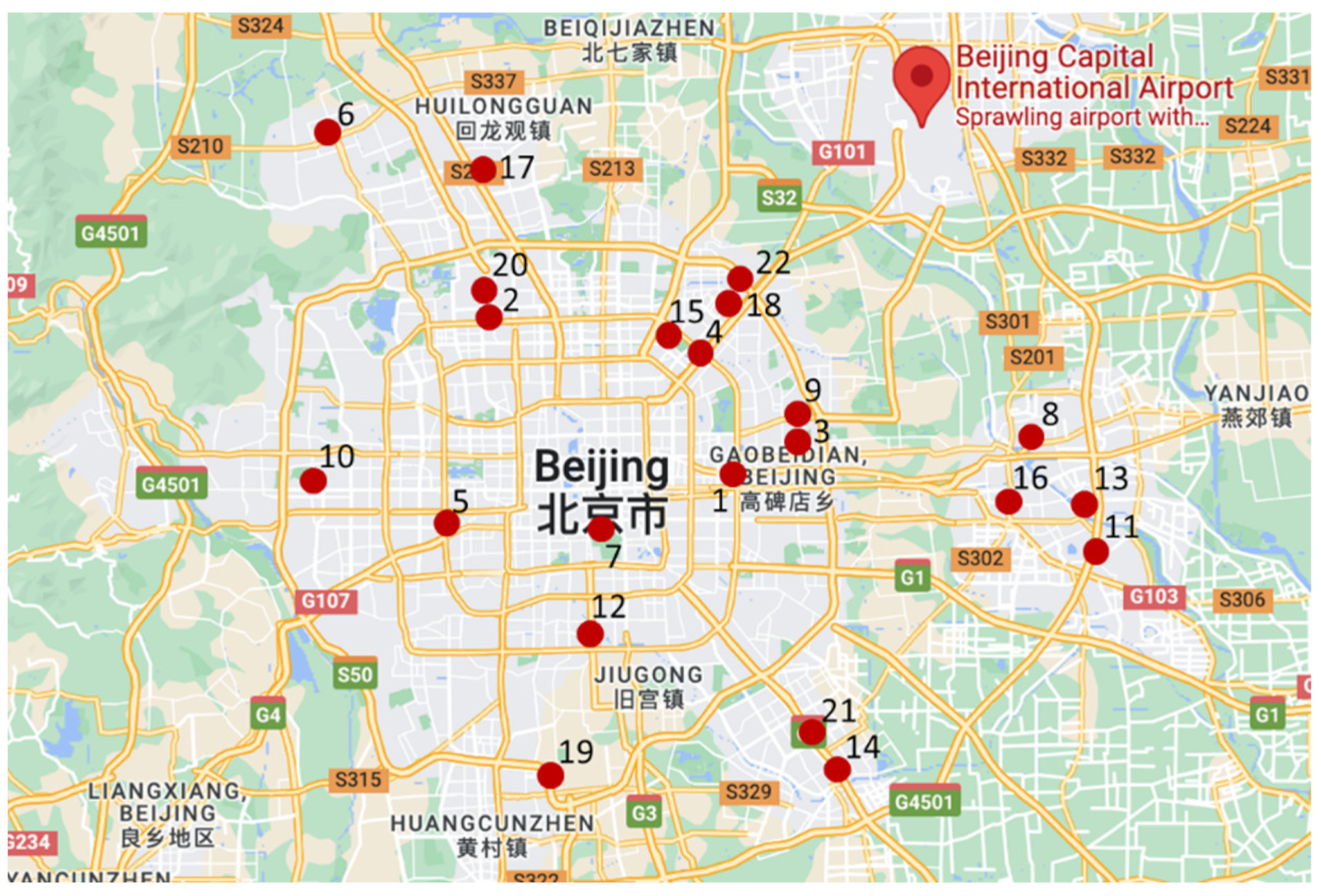
For the joint optimization of allocations and relocations in a two-operator carsharing system, case studies are based on historical order data provided by a carsharing company in Beijing. The total number of orders (also known as the user travel demand) per day is 1863 on average. In Figure 2, red dots indicate the locations of 22 commonly used stations, and they are numbered.

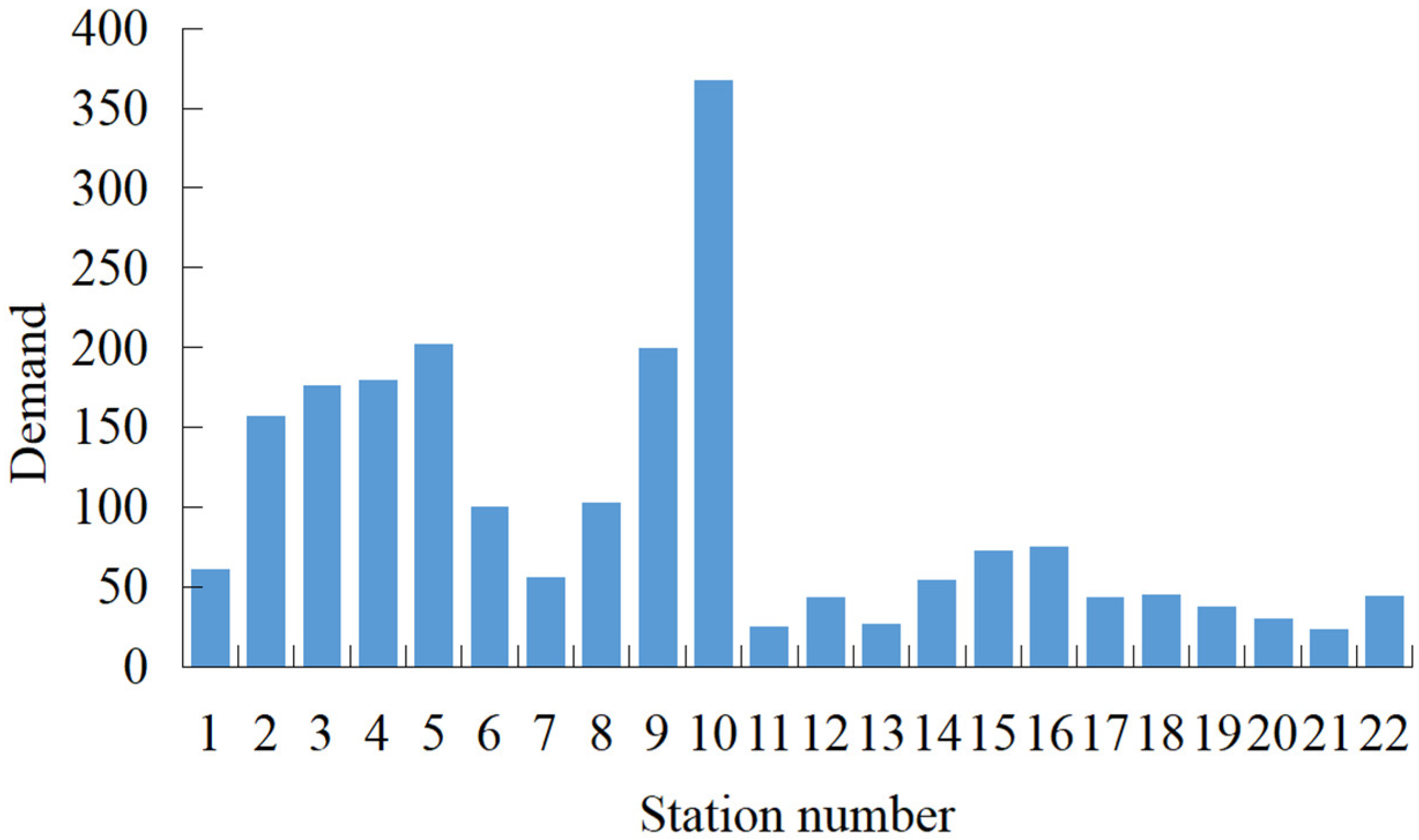
The operational period (06:00 to 24:00) is divided into 18 time steps with one-hour duration. 06:00 to 07:00 corresponds to the 1st time step, and so on, and 23:00 to 24:00 is the 18th time step. The demand distribution of each station is shown in Figure 3, and it is clear that demand varies greatly from station to station.

Assuming operators provide the same type of shared cars, the related parameters are taken with the same values. The depreciation cost $C_f$ per car per time step and maintenance cost $C_{mf}$ per parking space per day are CNY 17 and CNY 12, respectively [11]. Gas consumption $C_g$ per car per time step is CNY 9.2, and the relocation cost $C_r$ per time step is CNY 12, both taken from the market average. Operators charge users based on the mileages (CNY 1/km) and duration (CNY 6/time step) of each trip. The maximum number of parking spaces that can be allocated in total at each station is set to 100.

In addition, the parameters of the CAGA are outlined below. The maximum number of iterations $K$ and $G$ of the CAGA for the upper-level and lower-level models are both 100, population size $n$ and $m$ are both 50. When considering the user’s preferences, the travel utility function in Equation (8) consists of three components related to the travel cost, the number of available shared cars at the departing station, and the number of available parking spaces at the destination. Each part has corresponding weight coefficients; they are ${\gamma }_1$, ${\gamma }_2$, and ${\gamma }_3$, respectively, and all are taken as 1, which means that the three parts are equally important.

By comparing the indicators of carsharing systems with one operator and two operators, the impact of considering the interaction between operators on the performance of the carsharing system is explored, including the revenue (profit and various costs), allocations of parking spaces and shared cars, and demand satisfaction. The models constructed for each carsharing system were run 10 times with the CAGA, and the average value of each indicator was taken for analysis. Therefore, the decision variables are decimals.

(1)

Single-operator carsharing systems

The upper-level model of the bilevel programming model can be directly selected as the joint optimization model of allocations and relocations for the single operator. It consists of the objective function (13), allocation constraints about shared cars (14)–(16) and parking spaces (1), constraints related to demand satisfaction (10), and constraints about decision variables of the leader (17)–(19).

(2)

Two-operator carsharing systems

Based on whether users’ preferences are considered, the carsharing system can be divided into two categories below.

(i)

Without considering users’ preferences

Under this circumstance, the upper-level model includes objective function (13), allocation constraints about shared cars (14)–(16) and parking spaces (1), constraints (10) related to demand satisfied by the leader (where $y=l$), and constraints about the decision variables of the leader (17)–(19).

The lower-level model includes objective function (20), allocation constraints about shared cars (21)–(23) and parking space (2), constraints about the demand (10) satisfied by the follower (at this time $y=f$), and decision variable Constraints (24)–(26).

(ii)

Considering users’ preferences

An integer nonlinear bilevel programming model is built to describe this condition. Demands satisfied by the leader and the follower are constrained to be (7)–(9), with $y=l$ in the upper-level model and $y=f$ in the lower-level model, respectively.

The impact of the interactions between operators on the allocations of each operator will be discussed later by comparing indicators of each operator in carsharing systems with one operator and two operators.

4.2. Performance of the Two-Operator Carsharing System

Considering a two-operator carsharing system without considering users’ preferences, the impact of considering two operators is explored by comparing it with the single-operator carsharing system. All indicators are listed in

Table 5. Index comparison of different carsharing systems.

Indicators	Single Operator	Two Operators
		The Leader (Growth Rate %)	The Follower (Growth Rate %)
Revenue (CNY)	4714	4117.8 (−12.65)	2769.5 (−41.25)
Profit (CNY)	3316.7	2833.0 (−14.58)	1730.5 (−47.82)
Relocation cost (CNY)	161.1	186.6 (15.79)	226.8 (40.79)
Depreciation cost of sharing cars (CNY)	527.0	494.7 (−6.13)	421.2 (25.81)
Maintenance cost of parking spaces (CNY)	709.2	603.6 (−14.89)	409.2 (−40.61)
Satisfied demands	135.8	127.5 (−6.11)	85.1 (−37.33)
Number of sharing cars	31.0	29.1 (−6.13)	23 (−25.81)
Number of parking spaces	59.1	50.3 (−14.89)	35.1 (−40.61)
Number of relocations	3.9	4.3 (10.26)	4.9 (25.64)
Average demand per car satisfies	4.4	4.4 (0.00)	3.7 (−15.54)
Average time steps per user takes	2.33	2.21 (−4.98)	2.28 (−2.08)
Average profit per car makes	106.99	97.31 (−9.01)	75.24 (−29.68)
Average profit per parking space brings	56.12	56.32 (0.36)	49.3 (−12.15)

. The percentages in parentheses in the leader and the follower columns are the growth rate in each indicator for the leader or the follower compared to the operator in the single-operator carsharing system (named the single operator). Revenue is the cost paid by users and corresponds to the operator’s income; profit is the difference between revenue and all costs the operator paid; relocation cost is the fee paid by the operator during relocations.

(1)

Revenue and costs

Compared to the single-operator carsharing system, there is 12.65% less revenue and 14.58% less profit for the leader. Because the leader allocates fewer cars (6.13%) and parking spaces (14.89%), 6.11% less demand is met consequently. It indicates that the joining of the follower has an impact on the leader. In addition, the follower’s profit is much lower than the leader, showing that the leader has a great advantage in profitability, but the follower can also achieve a certain profit.

The leader and the follower allocate fewer sharing cars and parking spaces compared to the single operator, so depreciation costs and maintenance costs are also reduced. The number of relocations performed by the leader and the follower increased by 10.26% and 25.64%, respectively.

In the two-operator carsharing system, each operator’s profit (CNY 3316.7) is lower than that of the single-operator carsharing system, the total profit of both operators is much higher (CNY 4563.5). The number of shared cars and parking spaces allocated by each operator is reduced. In contrast, the total numbers are significantly increased. More demands can be met in this way (from 135.8 that can be met by the single operator to 212.6 by two operators), resulting in higher revenue for the overall carsharing market.

(2)

Allocations

As seen in Table 5, the average number of parking spaces allocated by the leader is 50.3, 8.8 fewer than the single operator. The number of sharing cars remained essentially the same. In addition, the leader brings an average profit of CNY 97.31/car, slightly lower than the single operator’s profit (CNY 106.99/car). The follower brings CNY 75.24 profit per car, much lower than the single operator.

In terms of the performance of shared cars, the follower can meet an average of 3.7 demands per car, slightly lower than the leader (4.4 demands/car). The leader can meet the same number of demands per car as the single operator. It suggests that the leader’s car utilization rate does not decrease significantly with the joining of the follower. The average trip duration for users choosing the follower (2.28 h) is slightly higher than that of users who choose the leader (2.21 h), and both of them are slightly lower than the average trip duration in single-operator carsharing systems (2.33 h).

Figure 4 shows the allocation details at each station. The black dash corresponds to the allocation of the single-operator carsharing system, and the bar graph shows the allocations of the two-operator carsharing system. By comparing the overall trends of the dashboard and bar graphs, it is clear that the two systems share similar allocations at each station.

(3)

Demand satisfaction

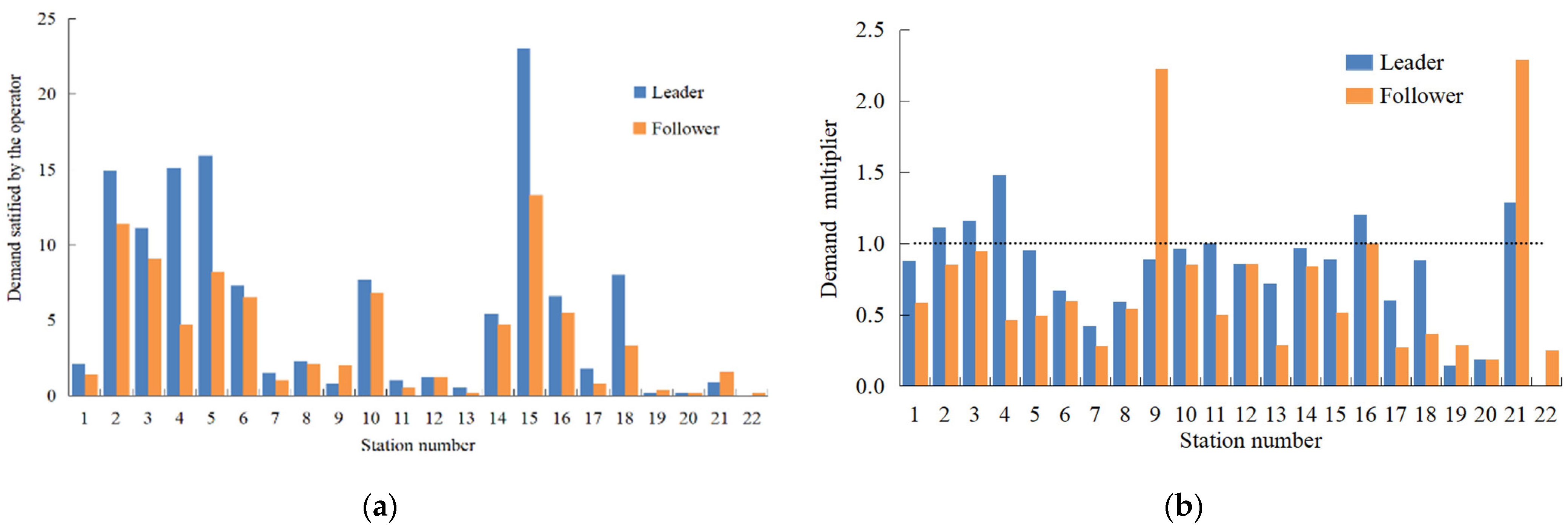
Figure 5a shows the demands satisfied by operators at each station. Combined with the distribution of parking spaces in Figure 4a, it is evident that allocations are closely related to demand satisfaction. The demand multiplier in Figure 5b is the ratio of demand satisfied by the leader or the follower to the demand satisfied by the single operator. The dashed line is the reference line corresponding to the demands that are satisfied by the single operator. When the demand multiplier is above the dashed line, which means that the demand satisfied by the leader or the follower is higher than that of the single operator, and vice versa. It can be seen that neither the leader nor the follower satisfies higher demand than the single operator at most stations. This phenomenon is consistent with the results in Table 5, where the average demand that can be satisfied by the single operator is 135.8, and 127.5 and 85.1 by the leader and the follower, respectively.

Overall, more demands can be satisfied when there are more operators. Compared to the single operator, the joining of the follower lowers demands and profit that the leader can satisfy to some extent. However, the leader’s profit remains much higher than the follower.

4.3. Impact of Considering Users’ Preferences

Users’ preferences are related to travel costs, the number of available shared cars at the departing station, and the number of available parking spaces at the arrival station. When one operator has more available cars at the starting station and more available parking spaces at the destination, users are more likely to choose the operator to complete the trip. By comparing the carsharing systems with and without considering users’ preferences, the operator’s revenue and costs, allocations, and users’ demand satisfaction are all analyzed.

(1)

Revenue and costs

Table 6. Values and growth rates of each indicator after considering users’ preferences.

Indicators	Leader		Follower
	Value	Growth Rate (%)	Value	Growth Rate (%)
Revenue (CNY)	15,202.8	222.50	7890.0	67.37
Profit (CNY)	9112.7	174.76	4520.6	36.30
Relocation cost (CNY)	0	−100.00	0	−100.00
Depreciation cost of sharing cars (CNY)	3406.8	546.45	1900.6	260.65
Maintenance cost of parking spaces (CNY)	2683.2	278.34	1468.8	107.11
Demand satisfied by the operator	498.2	266.84	305.5	124.98
Number of sharing cars	200.4	546.45	111.8	260.65
Number of parking spaces	223.6	278.34	122.4	107.11
Number of relocations	0	−100.00	0	−100.00
Average demand per car satisfies	2.49	−43.25	2.73	−37.62
Average time steps per user takes	2.24	−3.63	2.07	−11.05
Average profit per car makes	45.47	−57.50	40.43	−62.21
Average profit per parking space brings	40.75	−27.38	36.93	−34.19

shows the values of each indicator by considering users’ preferences, and the growth rate is obtained by comparing it to the single operator. For example, the leader’s profit growth rate = (leader’s profit − single operator’s profit)/single operator’s profit $\times$ 100%. Compared to the single-operator carsharing system, the leader’s revenue and profit improved significantly, increasing by 222.50% and 174.76%, respectively. The follower also achieves some improvements in revenue and profit, with growth rates of 67.37% and 36.30%, respectively. In addition, the profit of the leader remains higher than the follower, with its profit being about twice that of the follower.

From the perspective of costs, the depreciation cost of sharing cars and the maintenance cost of parking spaces all increase for both operators. The growth rates are 546.45% and 278.34% for the leader and 260.65% and 107.11% for the follower, respectively. The reason is that there is a big increase in the number of shared cars and parking spaces allocated by operators, as users prefer the operator with more available shared cars at the starting station and more available parking spaces at the arrival station. The relocation cost for both operators drops to 0, i.e., the corresponding number of relocations is 0. The reason is that each operator allocates a large number of shared cars and parking spaces to meet demands timely, so there is no need to relocate cars.

Table 7. Growth rates (%) by considering users’ preference (Comparing with the results found by without considering users’ preference).

Indicators	Leader	Follower
Revenue (CNY)	269.19	184.89
Profit (CNY)	221.67	161.23
Number of relocations	−100	−100
Number of sharing cars	588.66	386.09
Number of parking spaces	344.53	248.72
Demand satisfied by the operator	290.72	259.02
Average demand per car satisfies	−43.26	−26.14
Average time steps per user takes	1.42	−9.16
Average profit per car makes	−53.29	−46.26
Average profit per parking space brings	−27.64	−25.09

shows the growth rates of the leader and the follower when users’ preferences are considered, compared to the results when users’ preferences are not considered (e.g., the growth rate of the leader’s Revenue = (the leader’s Revenue with users’ preferences—the leader’s Revenue without users’ preferences)/the leader’s Revenue without users’ preferences). By considering users’ preferences, the leader’s revenue and profit both increase by at least 200%, and corresponding indicators also increase by more than 160% for the follower. This is due to the significant increase in the number of shared cars and parking spaces; the corresponding growth rates are 588.66% and 344.53% for the leader and 386.09% and 248.72% for the follower, respectively. At the same time, the demands met by the leader and the follower increased by 290.72% and 259.02%, respectively. It shows that the number of shared cars and parking spaces allocated by operators increases significantly after considering users’ preferences, and the demands met by sharing cars also increase a lot, leading to a big increase in profit. However, this is a significant drawback of considering users’ preferences, as the excessive number of shared cars and parking spaces allocated leads to a decrease of about 50% in profit per car and more than 20% in profit per parking space.

Table 8. Proportion of each cost to revenue (%).

Indicators	Single Operator	Without Users’ Preferences		With Users’ Preferences
		Leader	Follower	Leader	Follower
Profit	70.36	68.80	62.48	59.94	57.30
Relocation cost	3.42	4.53	8.19	0.00	0.00
Depreciation cost of sharing cars	11.18	12.01	14.12	22.41	24.09
Maintenance cost of parking spaces	15.04	14.66	15.21	17.65	18.62
Profit ratio to cost	188.54	220.49	166.55	149.63	134.17

shows percentages of each cost-to-revenue and profit ratio to cost. The latter refers to the ratio of profit to the total cost each operator paid. The total cost includes relocation cost, depreciation cost of shared cars, and maintenance cost of parking spaces. The higher the ratio, the more profitable the operator is.

When users’ preferences are not considered, the leader has the highest percentage of profit, up to 70.36%, as well as the highest profit ratio to cost, 220.49%. The two indicators of both operators are lower than the corresponding values of the single operator, and the follower is the lowest. It indicates that the profitability of each operator decreases after taking into account the users’ preference from the perspective of the profit ratio to cost only.

(2)

Allocations

As seen in Table 6, compared to the single operator, shared cars allocated by both operators drastically increase by 546.45% and 260.65%, respectively, when users’ preferences are considered. Demand per car meets decreases by an average of 43.25%, indicating a decrease in car utilization. The profit per car makes decreases by 57.50%, and the profit per parking space brings also decreases by 27.38% on average. It reveals that users’ preferences have a significant impact on the profitability of each operator.

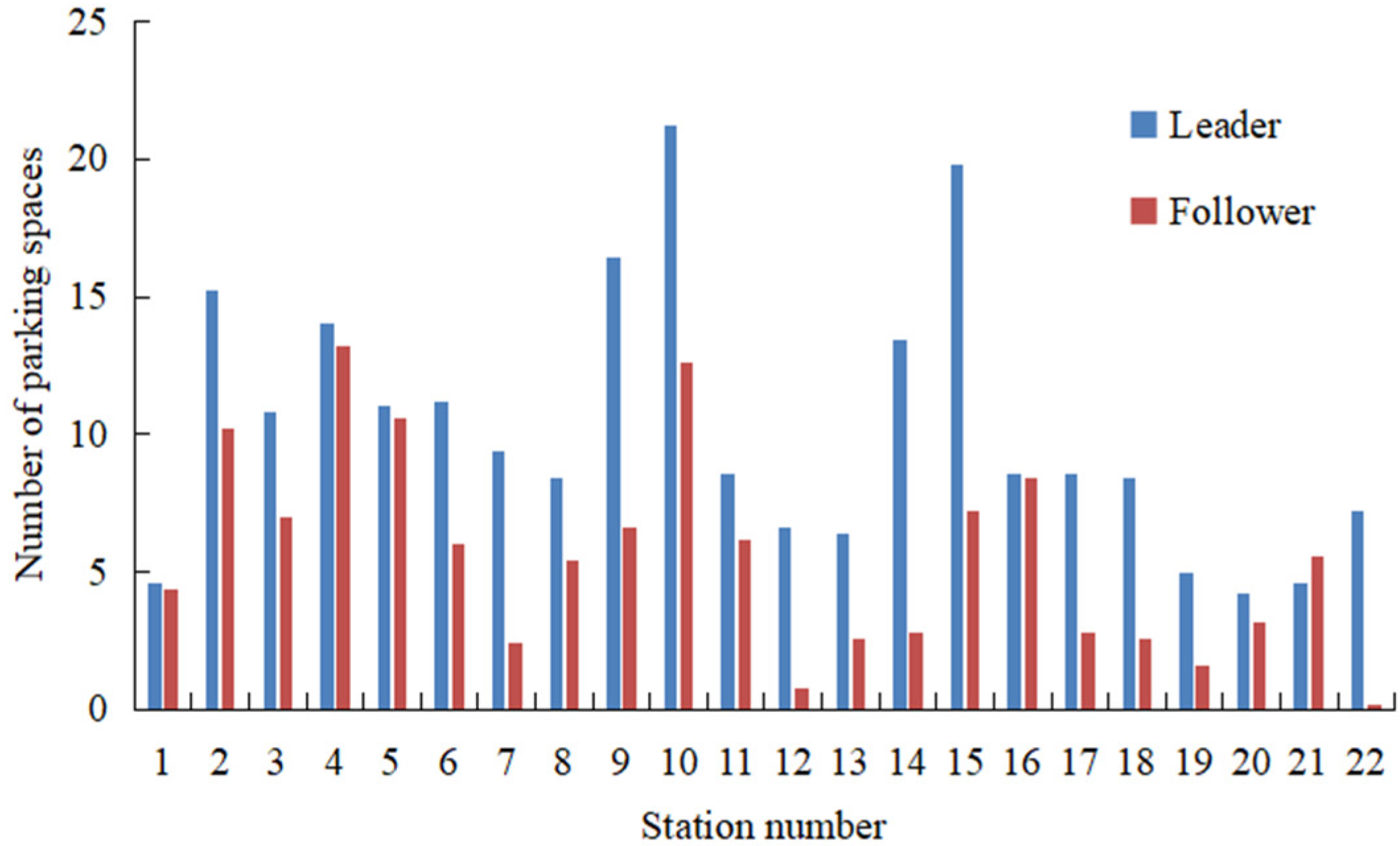
Figure 6 shows the allocation of parking spaces at each station in two-operator carsharing systems after considering users’ preferences. It shows that the leader allocates more parking spaces than the follower at most stations. The leader allocates more parking spaces to meet more demands. The total number of parking spaces that can be allocated to each station is limited, so the follower has fewer parking spaces to allocate.

(3)

Demand satisfaction

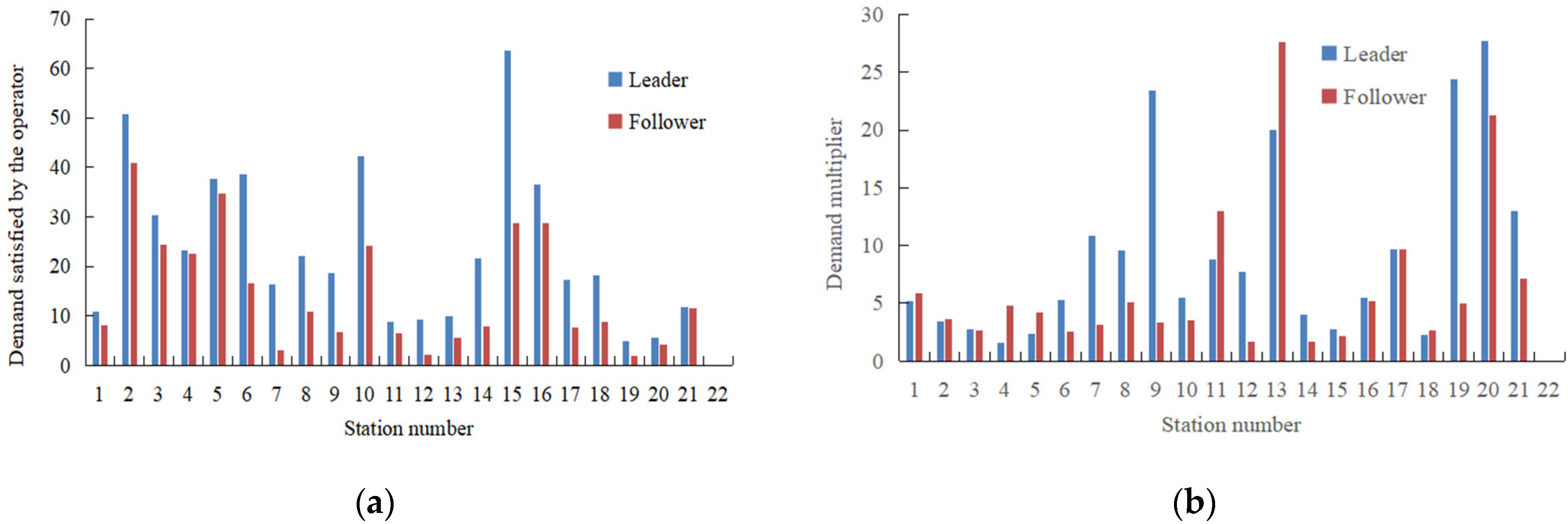
Figure 7 shows the demand satisfaction after considering users’ preferences. The follower satisfies no more demands than the leader at each station (Figure 7a). Figure 7b shows the demand multiplier, which is the ratio of the demand satisfied by the leader or the follower at each station to the corresponding value taken by the single operator. The dashed line is the reference line, indicating the demand satisfaction of the single operator. The demand multipliers for the leader and the follower are all much higher than 1 at most stations and even up to 20. While in Figure 5, each operator cannot satisfy more demands than the single operator at most stations without considering users’ preferences. This phenomenon suggests that operators can significantly satisfy more demands at most stations by considering users’ preferences.

Under this condition, demands per car can satisfy by the leader and the follower decrease by 43.26% and 26.14%, respectively (Table 7). In contrast, without considering users’ preferences, the demands each car satisfies on average by the leader is the same as that of the single operator (Table 4 and Table 5), but the follower decreases (15.54%). It means that considering users’ preferences can significantly reduce the car utilization rate.

In summary, the advantage of considering users’ preferences is that each operator can satisfy more demands, and profits are substantially higher. At the same time, the leader can receive more profit than the follower, and the follower’s profit is much higher than the single operator. However, disadvantages are also evident, such as that both operators allocate more parking spaces and sharing cars, resulting in significantly higher depreciation costs for shared cars and maintenance costs for parking spaces as well. In addition, the car utilization rate is not high with no relocations, while the profit per car and per parking space can bring to the operator decreases significantly.

5. Conclusions

It is common for multiple carsharing operators to coexist in carsharing systems. Furthermore, the performance of this kind of system is rarely studied. A two-operator carsharing system is taken as an example, assuming that the operator joins first as the leader and another joins later as the follower. The interactions between operators are considered to be a Stackelberg game, where the operators influence each other regarding limited parking spaces and demands. A bilevel programming model is constructed to describe the joint optimization of allocations and relocations. The allocations of shared cars and parking spaces, demand satisfaction, and relocations of each operator are considered. Then, a customized adaptive genetic algorithm (CAGA) is proposed to solve the model according to its characteristics. Finally, based on historical order data of a carsharing company in Beijing, a single-operator carsharing system is used as a reference to study the impact of considering the mutual influence of operators and users’ preferences.

The main conclusions drawn by this study are as follows:

(1)

It is necessary to study the interactions between the operators.

The interactions between the operators lead to lower profits for the leader (14.58%) and the follower (47.82%) than that of the single operator. While the total demands and profits obtained by the two operators significantly increased by 56.55% and 37.59%, respectively. It indicates that the interactions between the operators contribute to the overall development of the carsharing market.

(2)

Users’ preferences have a major impact on the performance of each operator.

Both operators are severely impacted by users’ preferences, especially the leader. For the leader, demands satisfied by shared cars and profit separately increase by 266.84% and 174.76%, and the number of shared cars and parking spaces increases substantially by 588.66% and 344.53%, respectively. The average profit per car or per parking space can make all decrease. Indicators of the follower also show similar changes to those of the leader, while all rates are slightly lower.

There are still many aspects that can be improved based on this research. For simplicity, this work only takes the carsharing system with two operators as an example, but there are more operators that coexist in reality. The interaction mechanism of operators would be much more complex. Further study can be undertaken based on this research. Moreover, only one type of user preference is considered. Future studies should discuss what factors should be considered and the weighting of these factors.

References

1. Li, M.; Zeng, Z.; Wang, Y. An innovative car sharing technological paradigm towards sustainable mobility. J. Clean. Prod. 2021, 288, 125626. [Google Scholar] [CrossRef]
2. Lu, R.; Zhao, X.; Wang, Y. A Tailored Pricing Strategy for Different Types of Users in Hybrid Carsharing Systems. Algorithms 2022, 15, 172. [Google Scholar] [CrossRef]
3. Martin, L.; Minner, S.; Pocas, D.; Schulz, A.S. The Competitive Pickup and Delivery Orienteering Problem for Balancing Car-Sharing Systems. Transp. Sci. 2021, 55, 1232–1259. [Google Scholar] [CrossRef]
4. Cheng, Y.; Chen, X.; Ding, X.; Zeng, L. Optimizing location of car-sharing stations based on potential travel demand and present operation characteristics: The case of Chengdu. J. Adv. Transp. 2019, 2019, 7546303. [Google Scholar] [CrossRef] [Green Version]
5. Li, W.; Li, Y.; Fan, J.; Deng, H. Siting of Carsharing Stations Based on Spatial Multi-Criteria Evaluation: A Case Study of Shanghai EVCARD. Sustainability 2017, 9, 152. [Google Scholar] [CrossRef] [Green Version]
6. Becker, H.; Ciari, F.; Axhausen, K.W. Comparing car-sharing schemes in Switzerland: User groups and usage patterns. Transp. Res. Part A Policy Pract. 2017, 97, 17–29. [Google Scholar] [CrossRef] [Green Version]
7. Balac, M.; Becker, H.; Ciari, F.; Axhausen, K.W. Modeling competing free-floating carsharing operators—A case study for Zurich, Switzerland. Transp. Res. Part C Emerg. Technol. 2019, 98, 101–117. [Google Scholar] [CrossRef] [Green Version]
8. Hu, L.; Liu, Y. Joint design of parking capacities and fleet size for one-way station-based carsharing systems with road congestion constraints. Transp. Res. B-Methodol. 2016, 93, 268–299. [Google Scholar] [CrossRef]
9. Sai, Q.; Bi, J.; Chai, J. Optimal model for carsharing station location based on multi-factor constraints. Algorithms 2020, 13, 43. [Google Scholar] [CrossRef] [Green Version]
10. Guo, H.; Chen, Y.; Liu, Y. Shared autonomous vehicle management considering competition with human-driven private vehicles. Transp. Res. Part C Emerg. Technol. 2022, 136, 103547. [Google Scholar] [CrossRef]
11. Huang, K.; Correia, G.H.D.A.; An, K. Solving the station-based one-way carsharing network planning problem with relocations and non-linear demand. Transp. Res. C Emerg. Technol. 2018, 90, 1–17. [Google Scholar] [CrossRef]
12. Deza, A.; Huang, K.; Metel, M.R. Charging station optimization for balanced electric car sharing. Discret. Appl. Math. 2020, 308, 187–197. [Google Scholar] [CrossRef] [Green Version]
13. Xu, M.; Meng, Q.; Liu, Z. Electric vehicle fleet size and trip pricing for one-way carsharing services considering vehicle relocation and personnel assignment. Transp. Res. B-Meth. 2018, 111, 60–82. [Google Scholar] [CrossRef]
14. Huang, K.; An, K.; Correia, G.H.D.A. Planning station capacity and fleet size of one-way electric carsharing systems with continuous state of charge functions. Eur. J. Oper. Res. 2020, 287, 1075–1091. [Google Scholar] [CrossRef]
15. Nourinejad, M.; Roorda, M.J. A dynamic carsharing decision support system. Transp. Res. E-Log. 2014, 66, 36–50. [Google Scholar] [CrossRef]
16. Yang, S.; Wu, J.; Sun, H.; Qu, Y.; Wang, D.Z.W. Integrated optimization of pricing and relocation in the competitive carsharing market: A multi-leader-follower game model. Transp. Res. Part C Emerg. Technol. 2022, 138, 103613. [Google Scholar] [CrossRef]
17. Fernández, J.; Boglárka, G.; Redondo, J.L.; Ortigosa, P.M.; Arrondo, A.G. A planar single-facility competitive location and design problem under the multi-deterministic choice rule. Comput. Oper. Res. 2017, 78, 305–315. [Google Scholar] [CrossRef] [Green Version]
18. Ma, H.; Guan, X.; Wang, L. A single-facility competitive location problem in the plane based on customer choice rules. J. Data Inf. Manag. 2020, 2, 323–336. [Google Scholar] [CrossRef]
19. Beresnev, V. Branch-and-bound algorithm for a competitive facility location problem. Comput. Oper. Res. 2013, 40, 2062–2070. [Google Scholar] [CrossRef]
20. Beresnev, V.L. On the competitive facility location problem with a free choice of suppliers. Autom. Remote Control 2014, 75, 668–676. [Google Scholar] [CrossRef]
21. Beresnev, V.; Melnikov, A. Exact method for the capacitated competitive facility location problem. Comput. Oper. Res. 2018, 95, 73–82. [Google Scholar] [CrossRef]
22. Nasiri, M.M.; Mahmoodian, V.; Rahbari, A.; Farahmand, S. A modified genetic algorithm for the capacitated competitive facility location problem with the partial demand satisfaction. Comput. Ind. Eng. 2018, 124, 435–448. [Google Scholar] [CrossRef]
23. Lin, Y.H.; Tian, Q. Generalized Benders decomposition for competitive facility location with concave demand and zone-specialized variable attractiveness. Comput. Oper. Res. 2021, 130, 105236. [Google Scholar] [CrossRef]
24. Kress, D.; Pesch, E. Competitive location and pricing on networks with random utilities. Netw. Spat. Econ. 2016, 16, 837–863. [Google Scholar] [CrossRef]
25. Jakobović, D.; Golub, M. Adaptive genetic algorithm. J. Comput. Inf. Technol. 1999, 7, 229–235. [Google Scholar]
Figure 1. Flow chart of the population initialization (taking the upper-level model as an example).
Sustainability 14 15308 g001
Figure 2. Schematic diagram of the distribution of a carsharing system in Beijing.
Sustainability 14 15308 g002
Figure 3. Demand distribution of each station.
Sustainability 14 15308 g003
Figure 4. Distributions of parking spaces and sharing cars at each station; (a) Parking spaces; (b) Sharing cars.
Sustainability 14 15308 g004
Figure 5. Demands met by the leader and the follower at each station; (a) Demand; (b) Demand multiplier.
Sustainability 14 15308 g005
Figure 6. Distribution of parking spaces at each station considering users’ preferences.
Sustainability 14 15308 g006
Figure 7. Distribution of the demand satisfaction considering users’ preferences; (a) Demand; (b) Demand multiplier.
Sustainability 14 15308 g007