Multi-Step Crude Oil Price Prediction Based on LSTM Approach Tuned by Salp Swarm Algorithm with Disputation Operator

Abstract

The economic model derived from the supply and demand of crude oil prices is a significant component that measures economic development and sustainability. Therefore, it is essential to mitigate crude oil price volatility risks by establishing models that will effectively predict prices. A promising approach is the application of long short-term memory artificial neural networks for time-series forecasting. However, their ability to tackle complex time series is limited. Therefore, a decomposition-forecasting approach is taken. Furthermore, machine learning model accuracy is highly dependent on hyper-parameter settings. Therefore, in this paper, a modified version of the salp swarm algorithm is tasked with determining satisfying parameters of the long short-term memory model to improve the performance and accuracy of the prediction algorithm. The proposed approach is validated on real-world West Texas Intermediate (WTI) crude oil price data throughout two types of experiments, one with the original time series and one with the decomposed series after applying variation mode decomposition. In both cases, models were adjusted to conduct one, three, and five-steps ahead predictions. According to the findings of comparative analysis with contemporary metaheuristics, it was concluded that the proposed hybrid approach is promising for crude oil price forecasting, outscoring all competitors.

1. Introduction

The most robust economies globally have become more vulnerable to oil price spikes due to armed conflicts, as the world witnessed in 2022. This indicates that the economic model derived from the supply and demand of crude oil prices is a significant influence factor measuring the world’s economic development and sustainability. For instance, the world’s largest oil importer, China, experiences squeezed consumer spending and lowered corporate profitability due to the impact of armed conflicts in Europe. Since the financial crisis in 2018, many internal and external factors, such as the change in the geopolitical environment, conflicts between countries, trade sanctions, the complexity and diverse nature of influencing factors on oil price prediction, etc., have made the prediction models highly non-reliable. The volatility of crude oil prices coupled with inflation strongly influences individual and corporate financing and investment decisions causing damage to global economic development. Therefore, it is essential to mitigate the crude oil price volatility risk by analyzing the associated metrics influencing simple oil price forecasting using machine learning to attain accurately predicted results.

Price prediction is an easy process, to begin with. However, the results may not be as accurate as they should be because some of the excluded factors may also be important in explaining the movement of prices. Additionally, geopolitical dynamics can affect oil prices. Markets tend not to be globalized but rather becoming regionalized due to the influence of geopolitical factors [1,2]. Accordingly, crude oil prices are nonlinear time series and highly volatile. As [3] examined the factors for natural oil price prediction and identified that the influence factors and their impact magnitude have changed over the period. With this changing environment, traditional approaches for price prediction may not serve the purpose as accurately as expected. That is why several studies that have attempted to forecast the price could not successfully bring the accuracy of their predicted outcomes.

To tackle crude oil price prediction, with a more refined accuracy, novel approaches are needed, that apply the latest technologies to the task at hand. As stated, predicting crude oil prices is a very challenging, yet potentially extremely lucrative endeavor. Artificial intelligence (AI) is a promising branch of computer science, that models learning processes observed in biological brains and groups of organisms, to address and adapt to resolving complex tasks in a changing environment. By developing and exploring machine learning (ML) models, which is a branch of AI, researchers have improved the way complex tasks are handled. Additionally, another promising member of the AI family are metaheuristics optimizers, such as swarm intelligence, that simulate group behaviors observed in nature and they are also capable of resolving non-deterministic polynomial hard (NP-hard) problems, considered impossible to accomplish with traditional deterministic methods.

However, it is important to note that the performance of ML algorithms is heavily dependent on their configuration. Many algorithms need to remain flexible enough to address a general set of problems, but also to target a specific challenge. Adaptations (tuning) of ML models for a concrete task at hand are performed by tuning its un-trainable parameters, which are referred to as hyper-parameters. The hyper-parameters define the intricacies of the algorithm. However, finding its optimal (sub-optimal) values for specific tasks is a complex NP-hard challenge.

To address this, researchers have developed approaches to automate the process of hyper-parameter selection, called hyper-parameters tuning. Since hyper-parameter tuning can be formulated as a typical optimization problem, researchers have employed various optimization algorithms to select the optimal (sub-optimal) hyper-parameter values and attain the best possible performance for the model. A particularly well-performing group of algorithms that excels in tackling optimization tasks is swarm intelligence. Often used to address complex, and even NP-hard problems, this group of algorithms is particularly popular among researchers, due to its relative simplicity and not-so-high computational demands. With this in mind, this work explores the use of a particularly interesting algorithm that emulated the behavior of salp foraging for food, the salp swarm algorithm (SSA) [4], which was adopted for ML hyper-parameters optimization.

However, besides tuning the model for time-series forecasting, facing problems where output doesn’t only depend on previous values, but also its order, is also influenced by some additional challenges. Time-series are complex and non-linear dependencies between data points and as such interpreting them is complex. Time series data will often show trends and patterns in the way it changes. However, while some trends are apparent, certain more subtle trends are harder to detect. A similar problem is present in the field of signal processing, where researchers often need to extract signal components from complex compound inputs. To address these issues, methods for decomposing data into sub-components have been developed. The variational mode decomposition (VMD) [5] is a relatively novel algorithm that shows great promise when tackling complex series of data. By treating and formulating financial data as a signal, data decomposition methods can be applied to deter, observe and extract trends in price changes. This approach allows for work with larger datasets or simpler components rather than with one exceedingly complex signal.

It is important to note that a noticeable research gap is present in modern literature from the domain of tacking crude oil price prediction as a pressing economical task, by ML approaches. Furthermore, the use of decomposition methods for data processing has been tackled by very few researchers. A notably interesting approach has been proposed in [6], where VMD signal decomposition is efficiently coupled with kernel extreme learning machine (KELM) for crude oil price forecasting. Therefore, this paper served as an inspiration for the research conducted in this work, while the motivation stems from the fact that this very important issue has not been enough investigated in the modern literature by applying ML models and that there is a lot of free space for improving forecasting accuracy.

Therefore, to tackle oil-price forecasting, this research employs a single layer long term short memory (LSTM) model, to create as simple as a possible neural network, capable of tackling this problem efficiently, from aspects of prediction accuracy and the use of computational resources. However, since the LSTM should be tuned for each specific time-series, the introduced modified SSA algorithm is utilized for LSTM hyper-parameters tuning challenge. It’s worthwhile mentioning that the previous research findings confirmed that the LSTM is very efficient when dealing with time-series data [7,8,9].

To ensure a more robust and accurate performance analysis, the proposed research is based on two experiments, that have been carried out. The first makes use of a simple LSTM network, while the second applied VMD to the data with the K components used as inputs for the LSTM. The second experiment adopts well-known TEI@I (integration of text mining, Econometrics, and intelligence) complex system research methodology [10], that employs a decomposition algorithm (in this case VMD) and a prediction model (in this case LSTM network).

Both experiments made predictions for crude oil prices one, three, and five steps ahead. The accuracy of prediction results has been evaluated based on the standard regression and time-series forecasting metrics. Additionally, a rigid comparative analysis was performed with evolved LSTM models by other state-of-the-art metaheuristics methods.

Simulations were carried out using West Texas Intermediate (WTI) real-world crude oil price data, that covers daily prices, for the period 2 January 1986–11 July 2022, not including weekends.

The scientific contributions of this work may be summarized as the following:

• A proposal of an improved version of the SSA designed to improve on the admirable performance of the original algorithm.
• The application of VMD decomposition technique to address crude oil time-series data complexity.
• Adjusting LSTM using the novel proposed swarm intelligence algorithm to improve performance when predicting directional trends in data components.
• Further investigating and filling the research gap from the crude oil price forecasting domain by applying hybrid methods between LSTM and swarm intelligence.

The remainder of this work is structured according to the following: Section 2 provides a look into works preceding this research, as well as the approaches involved in realizing it. The proposed improved swarm intelligence method is described in detail in Section 3. The experimental setup and dataset used in simulations are covered in Section 4, while the attained results with comparative analysis are discussed in Section 5. Finally, Section 6 presents a conclusion on the conducted research and discusses future work in the field.

2. Review of the Literature and Basic Background

In recent times, machine learning (ML) has been widely used in research in the field of economics and finance, where some predictions are to be executed to arrive at precise estimations. Crude oil price fluctuations are generally nonlinear and irregular, challenging researchers to predict future trends accurately. However, crude oil price prediction is an essential input variable for individuals, corporates, and government sectors for their financial planning. Considering this fact, [11] examined the application o fML and computational model to predict monthly crude oil prices. The results prove the effectiveness of the data and provide a better prospect for oil price prediction in the future.

As [12] argued that research accuracy depends on the relevance and correctness of information gathered and the algorithms employed. According to [13,14], ML has been the most sought-after predicting mechanism in finance and economics. Additionally, [15] has adopted ML models to predict stock prices.

According to [16], varied factors influence oil price fluctuations. The effects of these factors are much more complicated and dynamic. So, it is not easy to extend the results of a model predicting the oil prices now to a future period unless the model considers the dynamism of the effect of input variables. Thus, they tried the deep learning model approach to measure the movement of oil prices due to the nonlinear variables. The price data in the WTI crude oil markets validate the accuracy of the model results, which shows that the model provides a better prediction.

As [17] examined the appropriateness of artificial intelligence techniques in predicting oil prices. The prediction of oil prices is complex as their movement is highly irregular, which is very complex to predict. They examined the potential of AI in oil price prediction. They examined various models for oil price forecasting, covering thirty-five research papers published from 2001 to 2013, based on the following parameters: (a) input variables, (b) input variables selection method, (c) data characteristics, (d) forecasting accuracy, and (e) model architecture. Their results highlighted the appropriateness of AI methods used in complex oil price-related studies and the specific shortcomings. They suggested how to improve them in the future.

Notably, research [18] has predicted the stock prices of construction companies in Taiwan using a promising nonlinear prediction model. Researchers [19] analyzed extensive information using machine learning algorithms to examine the movement of stock market indices. Work presented in [20] examined two models: the generic deep belief network model and the adaptive neural fuzzy inference system for predicting crude oil prices. The results of these two models were compared with the traditional strategies such as a naïve strategy, a moving average convergence divergence model, and an auto-regressive moving average (MV) model. The proposed two models achieved better results comparatively, providing higher accuracy.

2.1. Artificial Neural Networks and Long Short Term Memory

Artificial neural networks (ANN) [21] form the basis of deep learning methods. Heavily inspired by learning mechanisms observed in human brains, this group of algorithms leverages computing power to mimic the mechanisms by which neurons transmit and interpret signals between each other. These algorithms are capable of inferring correlations between data through a training process, effectively learning by example. This ability makes them especially attractive for tackling complex non-linear problems.

Notwithstanding that many efficient deep learning models exist, the long short-term memory (LSTM) proved as one of the most promising models when tackling time-series forecasting challenges [7,8,19]. The LSTM allows the storage of information inside the network. This way, future outcomes are influenced by the results of previous inputs, which means they are suitable for time-series predictions. Cells in traditional networks are switched out for memory cells in hidden layers, therefore, allowing for the memory retention mechanism. Using input gates, output gates, and forget gates, memory cells can selectively store and release the data that goes through them.

Data first makes its way through the forget gate where a decision is made on whether to discard the memorized data from the memory cell. It can be described as per Equation (1).

$$f_t=\sigma (W_f{x}_t+U_f{h}_{t-1}+b_f)$$

(1)

in which $f_c$ marks the gate with the $[0, 1]$ range. The sigmoid function is represented by $\sigma$; while $W_f$, $U_f$ are variable weight matrices, $h_{t-1}$ defines the output of the previous LSTM block and $b_f$ is the bias vector.

The subsequent stem picks the data for storage within memory cells. The sigmoid function of gate $i_t$ selects renewed values determined by Equation (2).

$$i_t=\sigma (W_i{x}_t+U_i{h}_{t-1}+b_i)$$

(2)

in which $i_t$ has a $(0,1)$ range. The series of learnable parameters of an input gate are $b_i$, $W_i$, and $U_i$. Potential update vectors $C_t$ are computed by Equation (3)

$$C_t=tanh(W_c{x}_t+U_c{h}_{t-1}+b_c)$$

(3)

where $b_c$, $W_c$, $U_c$, similarly stand for a series of learnable parameters.

After the initial decision steps that select data to be stored, the given cell’s state $C_t$ is computed according to Equation (4)

$$C_t=f_t\odot C_{t-1}+i_t\odot C_t$$

(4)

with ⊙ signification and element-wise multiplication. Data determined for erasure is defined as $C_{t-1}$. Correspondingly, the data meant for storage is defined as $f_t\odot C_t$, where $f_t$ represents the forget gate. The novel information that will be stored in a memory cell $C_t$ is denoted as $i_t\odot C_t$.

By using the sigma function in regards to Equation (5), the output gate $o_t$ value that defines the hidden state $h_t$, with t representing the current iteration, can be calculated.

$$o_t=\sigma (W_o{x}_t+U_o{h}_{t-1}+b_o)$$

(5)

in which the range of $o_t$ is $(0,1)$, and $b_o$$W_o$ and $U_o$ stand for learnable parameters for the input gate. Lastly, the result of $o_t$ and $tanh$ value of $C_t$ is the output value $h_t$ in accordance with Equation (6)

$$h_t=o_t\odot tanh\left(C_t\right)$$

(6)

2.2. Variational Mode Decomposition (VMD)

By applying signal decomposition to a complex signal, its principal modes may be extracted via the use of VMD [5]. When applied to price data, this approach allows different band-limited intrinsic mode functions (IMF) to be extracted from the base data. These IMFs represent an observed sub-trend present in the original data. While resulting in a larger overall dataset, the components have a more regular shape, allowing algorithms to tackle them individually in a more effective manner. By determining relevant bands adaptively VMD estimates the corresponding modes concurrently, thus properly balancing errors between them.

Each mode may be defined according to Equation (7):

$$u_i\left(t\right)=A_i\left(t\right)cos\left[{\varphi }_i\left(t\right)\right]$$

(7)

where $u_i\left(t\right)$ represents the i-th amplitude-frequency modulation signal mode component, $A_i$ the current amplitude, and $cos\left[{\varphi }_i\left(t\right)\right]$ the phase.

The VMD approach leverages center frequency and bandwidth to extract different signal components. Every mode is compressed around a central pulsation ${\omega }_i$, while the bandwidth is estimated via the $L^2$ norm of the gradient. A more complete elaboration of the $L^2$ norm can be found in [22]. The composition process can be performed according to Equation (8)

$$\begin{array}{c}\hfill mi{n}_{\left\{u_i\right\},\left\{{\omega }_i\right\}}\left\{\sum _{i=1}^K{\displaystyle \parallel }{\partial }_t[\delta \left(t\right)+\frac{j}{\pi t}\ast u_i\left(t\right)]e^{-j{\omega }_{i}t}{{\displaystyle \parallel }}_2^2\right\}\\ \hfill s.t.x\left(t\right)=\sum _{i=1}^K{u}_i\left(t\right)\end{array}$$

(8)

with K representing the amount of modes, $\left\{u_i\right\}=\{u_1,u_2,\cdots ,u_i\}$ and $\left\{{\omega }_i\right\}=\{{\omega }_1,{\omega }_2,\cdots ,{\omega }_i\}$ are sets of estimated modes and their center frequencies. Further, $j^2=-1$, ${\partial }_t$ represents the gradient function, and $\delta \left(t\right)$ denotes the Dirac distribution.

Using the Lagrangian multiplier $\lambda$ along with the penalty factor ℵ, the constrained variational problem is transformed into an unconstrained one, that is described according to Equation (9):

$$\begin{array}{c}\hfill L(\left\{u_i\right\},\left\{{\omega }_i\right\},\lambda )=\aleph \sum _{i=1}^K\parallel {\partial }_t[\left(\delta \left(t\right)+\frac{j}{\pi t}\ast u_i\left(t\right)\right]e^{-j{\omega }_{i}t}{\parallel }_2^2+\left|\right|x\left(t\right)-\sum _{i=1}^K{u}_i\left(t\right){\left|\right|}_2^2+\langle \lambda \left(t\right),x\left(t\right)-\sum _{i=1}^K{u}_i\left(t\right)\rangle \end{array}$$

(9)

Alternating direction methods of multipliers are applied to locate a local minimum of the Lagrangian function. Estimated modes ${\widehat{u}}_i$ is determined according to Equation (10) while its central frequency ${\omega }_i$ is determined with respect to Equation (11):

$${\widehat{u}}_i^{n+1}\left(\omega \right)=\frac{\widehat{x}\left(\omega \right)-{\sum }_{j\ne i}{\widehat{u}}_j\left(\omega \right)+\frac{\widehat{\lambda }\left(\omega \right)}{2}}{1+2\aleph {(\omega +{\omega }_i)}^2},$$

(10)

$${\omega }_i^{n+1}=\frac{{\int }_0^{\infty }\omega {\left|{\widehat{u}}_i\left(\omega \right)\right|}^{2}d\omega }{{\int }_0^{\infty }{\left|{\widehat{u}}_i\left(\omega \right)\right|}^{2}d\omega }$$

(11)

where n determines the number of iterations. The $\lambda$ Lagrange operator is determined according to Equation (12):

$${\widehat{\lambda }}^{n+1}\left(\omega \right)={\widehat{\lambda }}^n\left(\omega \right)+\tau [\widehat{x}\left(\omega \right)-\sum _{i=1}^K{\widehat{u}}_i^{n+1}\left(\omega \right)]$$

(12)

with $\tau$ representing noise tolerance control parameter.This equation will be repeated until Equation (13) is fulfilled.

$$\sum _{i=1}^K\frac{\left|\right|{\widehat{u}}_i^{n+1}-{\widehat{u}}_i^n{\left|\right|}_2^2}{\left|\right|{\widehat{u}}_i^n{\left|\right|}_2^2}<\epsilon$$

(13)

Four control parameters are present in the VMD method. These include the noise tolerance $\tau$, convergence error $\epsilon$, the number of model components K, and finally the quadratic penalty factor ℵ. With parameters K and ℵ having a more significant effect on attained results.

2.3. Swarm Intelligence

Swarm intelligence presents a particularly powerful group of metaheuristic optimization algorithms, often inspired by groups observed in nature such as the artificial bee colony (ABC) [23], whale optimization algorithm (WOA) [24], firefly algorithm (FA) [25]. However, this is not always the case, as more abstract mathematical concepts have served as inspiration for several notable algorithms such as the sine cosine algorithm (SCA) [26] and arithmetic optimization algorithm (AOA) [27]. Best known for their ability to address complex tasks including NP-hard problems swarm intelligence algorithms are particularly popular among researchers for tackling optimization problems. It is important to note that due to the random nature inherent in the mechanisms of these algorithms, an optimal solution can never be guaranteed. However, with each successive iteration the odds of finding a true optima increase.

Algorithms from this group make use of populations of agents, that obey subsets of rules. This mechanism allows for complex intelligent behavior to occur on a global scale as agents strive towards a common goal guided by an objective function. The formulation of an objective function depends on the specific problem being addressed. Furthermore, it is important to note that despite admirable flexibility, there is no single approach that works best applied to all problems, this is further enforced by the no free lunch theorem [28]. Constant experimentation and adjustments are needed to further adjust and improve applications of swarm intelligence.

As such, much research and experimentation has been done with swarm intelligence algorithms with many optimization applications in several fields [29,30,31,32,33,34].

3. Proposed Method

This section first provides a brief overview of the original SSA metaheuristics, followed by its observed cons, and concludes with a detailed description of a modified approach proposed in this research.

It is noted that when the original SSA is described, notations from its introducing paper are preserved [4], while the approach used in this study uses slightly different notation, which is more adapted to commonly used practices in the metaheuristics literature, e.g., current iteration and a total number of iterations in a run are denoted as l and L, respectively, in the original SSA, while the method in this study uses notations t and T.

Moreover, despite the fact that the authors do not agree with introducing new terminology for each devised metaheuristics, the terms which are used in the original SSA paper [4], is also preserved, e.g., solutions are known as salps, the current best solution is referred as the leader, the second best as a follower, etc. Authors think that ’nature-inspired’ terminology should be avoided when new algorithms are introduced and that the uniform terminology from the metaheuristics domain should be followed.

3.1. Salp Swarm Algorithm

The SSA [4] algorithm is inspired by the foraging behaviors of salp. To find the safest route to the sustenance supply individual salps band together by creating a chain with their bodies connected. This mechanism is used as a model for exploration and exploitation. The former leader adapts positioning towards the direction of the sustenance supply which represents the current optimum.

Agent positions in population with size N in d-dimensional space is determined via two-dimensional matrix X as per Equation (14):

$$X_i=\left[\begin{array}{cccc}{x}_1^1& x_2^1& \cdots & x_d^1\\ x_1^2& x_2^2& \cdots & x_d^2\\ ⋮& ⋮& \cdots & ⋮\\ x_1^N& x_2^N& \cdots & x_d^N\end{array}\right]$$

(14)

With the sustenance supply defined as F, the leader`s position (best solution) in the j-th dimension is updated by the following function (15):

$$x_j^1=\left\{\begin{array}{c}{F}_j+c_1((u{b}_j-l{b}_j)c_2+l{b}_j),c_3\ge 0.5\hfill \\ F_j-c_1((u{b}_j-l{b}_j)c_2+l{b}_j),c_3<0.5,\hfill \end{array}\right.$$

(15)

where $x^1$ defines ladder positioning, $F_j$ marks the current optimal solution location, the upper and lower boundaries are defined by $u{b}_j$ and $l{b}_j$, $c_1$, $c_2$ and $c_3$ represent pseudo-random values in range $[0, 1]$.

Parameters $c_2$ and $c_3$ dictate step size and control should the position of the new solution be directed towards positive or negative infinity. Nevertheless, $c_1$ remains important since it directly dictates the ratio between exploration and exploitation. The $c_1$ can be determined according to Equation (16):

$$c_1=2e^{-{\left(\frac{4l}{L}\right)}^2},$$

(16)

in which the current iteration is labeled as l and L stands for maximum iterations in one run.

Follower positions are updated using Equation (17)

$$x_j^i=\frac{1}{2}a{t}^2+V_{0}t,$$

(17)

where $x_j^i$ represents i-th follower in the j-th dimension and $i\ge 2$. Annotation t labels time and $a=\frac{V_{final}}{V_0}$, i which $V=\frac{x-x_0}{t}$, and the initial speed is $V_0$.

Considering that time in all optimization processes based around iterations, the disparity between iterations is 1 and $V_0=0$ at the beginning, Equation (18) can be redefined as:

$$x_j^i=\frac{1}{2}(x_j^i+x_j^{i-1})$$

(18)

3.2. Cons of the Original Algorithm

Most basic optimization algorithms have some downsides, the SSA being no different. Observed deficiencies of the basic SSA in short are insufficient exploration, average exploitation power (conditional drawback), and intensification-diversification trade-off.

According to modern literature sources [35], an optimization algorithm might be bettered with minor modifications, e.g., small changes added to the search equation, additional mechanisms, and/or by imposing significant changes by hybridization with other methods For the needs of the present study, basic SSA was improved by adding a disputation operator, that performs a group search within the cluster of promising solutions.

Using the results of previous research [36], in addition to extensive experimentation using standard CEC2013 benchmark test functions [37] that were done specifically for this study, a conclusion was reached that the diversification process of basic SSA shows some shortcomings, leading to the inappropriate balance of intensification-diversification, with the dis-balance usually leaning towards exploitation.

3.3. Ssa with Disputation Operator

The SSA algorithm proposed in this manuscript tackles the observed flaws of the original SSA implementation by applying the disputation operator, proposed by the social network search (SNS) algorithm in [38]. This operator is used to guide the search within a chosen subgroup of solutions from the population. The original SNS has defined this process where the users of the social network are explaining and also defending their opinions on a certain topic with other network users. The users can also establish new groups for the elaboration of different topics. Consequently, it is possible to affect the users through other users’ opinions on specific topics. The mathematical formulation of this process is given by Equation (19) [38], which shows the update process of the solution x for the i-th parameter.

$$\begin{array}{cc}\hfill & x_{inew}=x_i+rand(0,1)\times (M-AF\times x_i)\hfill \\ \hfill & M=\frac{{\sum }_t^{N_r}{x}_t}{Nr}\hfill \\ \hfill & AF=1+round\left(rand\right),\hfill \end{array}$$

(19)

where $x_i$ describes the vector representing the view of $i-th$ user, $rand(0,1)$ stands for a random vector within the range $[0, 1]$ and M denotes the mean of views of users belonging to the commentator group. The $AF$ value represents the admission factor used as an indicator of the persistence of the users that hold to their opinions while discussing with other users and it can have integer values of 1 or 2. Function $round\left(\right)$ has a role to round the input to the nearest integer value, while $rand$ represents an arbitrary number within the range $[0, 1]$. Variable $Nr$ denotes the number of commentators or group size. Consequently, it can hold integer values between 1 and N, N representing the total number of the network’s users.

The parameter $AF$ controls the search step size, therefore impacting the trade-off between the intensification and diversification phases. In case the value of $AF$ is set to 2, the exploration is favored, while in the case of value 1, the disputation phase is supported, leading to intensified exploitation.

This work uses a modified disputation operator as described in the remaining of this section. The basic implementation of the SNS metaheuristics presumes that the first operand of $AF$ equation (Equation (19)) has been hardcoded to value 1, therefore the possible values $AF$ can take just 1 and 2. However, the extensive simulations with the original version of the algorithm have empirically shown that it is more convenient to define a larger initial step size that focuses on the exploration, and to decrease it at a slow pace over the iterations, to focus more on the exploitation process. Furthermore, it is more effective to regard the $AF$ as a continuous parameter, to enable metaheuristics search process fine-tuning.

Considering these observations, instead of determining the step size $AF$ by using Equation (19), the method presented in this paper uses one supplementary dynamic group search control parameter ($gsp$) and utilizes the Equation (20) to determine $AF$ in each round.

$$AF=gsp+round\left(rand\right).$$

(20)

where the $gsp$ parameter decreases dynamically in each iteration t, from its initial value of 2. This reflects the need to focus more on the exploration during the initial phases and shift the focus to exploitation in the later rounds. The proposed approach uses a fine-grained step size $AF$, that allows more accurate control of the search process than the basic SNS implementation.

Additionally, the introduced method incorporates a two-mode group search, that is implemented as follows: the first mode is performing the search within the group of $N_r$ randomly chosen solutions from the population, while the second mode is focused on the group of $N_b$ best solutions within the swarm. Both $N_r$ and $N_b$ are established in each iteration, as random values within the range [$1,N$]. The Equation (19) is utilized in both modes, while the step size is calculated as defined in Equation (20). The second mode is applied in later iterations to focus on the search process near the current best solutions, with the assumption that the algorithm has successfully converged to the optimal region of the search domain. The switching between modes 1 and 2 is performed by the control parameter $cmt$, labeled as change mode trigger, with respect to the termination condition.

Based on the empirical simulations, it was concluded that the basic SSA search mechanism is able to converge fast to the optimal solution in cases where the initial population was produced near the optimal regions. To give a chance to the basic SSA search and not increase significantly the complexity of the method, the proposed group search procedure is not initiated in early iterations, but after passing of $gss$ (group search start) iterations. In each iteration, if the condition for the group search is fulfilled, the proposed method produces a new individual $x_{new}$, and performs the greedy selection procedure between the produced solution and arbitrarily selected individual from the 50% of the worst solutions from population $x_{rnd\_worst}$.

The proposed method was dubbed SSA with disputation operator (SSA-DO), to reflect the implemented search mechanism. In addition, the proposed method makes use of three supplementary control variables, which all depend on the termination condition (either T, which represents the maximal number of iterations or the fitness function evaluation $FFEs$ count), while one among them has dynamic nature. Their values were determined empirically, as given in

Table 1. Settings of the important SSA-DO control parameters.

Parameter	Expression	Description
$gsp$	$gsp=gsp-\frac{t}{T}$	dynamic group search parameter, initially 2
$gss$	$gss=\frac{T}{3}$	group search start
$cmt$	$cmt=gss+\frac{T}{3}$	change mode trigger

.

To determine the complexity of the suggested SSA-DO approach, the complexity of the original SSA must be considered with respect to the $FFEs$. The $FFEs$ is a common way to establish the complexity of the metaheuristics algorithms, as stated in [39]. When compared to the basic SSA, the SSA-DO complexity is higher by only $(T-gss)$$FFEs$, since only one new individual is generated in every iteration after enabling the group search. This fact was taken into consideration when compared to other algorithms to provide a fair basis for analysis.

It should be noted here that a similar technique was recently suggested in [40], by the same research group. The approach given in [40] is replacing the latest worst individual $x_{worst}$ with the solution produced through the group search mechanism. Continued research has shown that in some cases it may lead to the loss of diversity, specifically, if the solutions that have better fitness than the latest $x_{worst}$ are dwelling in sub-optimal areas. Consequently, the work presented in this paper utilizes a different strategy.

Lastly, the introduced SSA-DO pseudo-code is presented in Algorithm 1.

Algorithm 1: The SSA-DO pseudo-code.

Set values for N and T parameters Set basic SSA control parameters Set specific SSA-DO parameters Initialize swarm $x_i(i=1,2,\cdots ,N)$ Initialize iteration counter, $t=0$ while$t<T$do    Determine best-performing agents    Designate F as the best solution    for All agents($x_i$) do      if $i==$ 1 then         Update best solution’s position according to Equation (15)      else         Update follower positions according to Equation (18)      end if    end for    Move all solutions from outside of boundaries back into the search space    if $t>gss$ then      if $t<cmt$ then         Produce new agent $x_{new}$ by utilizing the group search mode 1 operator      else         Produce new agent $x_{new}$ by applying group search mode 2 operator      end if      Perform greedy selection between $x_{new}$ and $x_{rnd\_worst}$    end if    Rank all solutions to find the current best agent    Update $C_1$ according to Equation (16)    Update $gsp$ as specified in Table 1 end while return Best solution

4. Experimental Setup

For the purpose of exhibited research two experiments have been conducted. The first experiment applied LSTM to predict crude oil prices from the original time-series, while the second experiment applied VMD to data before applying LSTM to the output results of the VMD (VMD-LSTM approach). For both experiments, a lag of 6 data points has been used for predictions, and 3 simulations, for one, three, and five steps (days) ahead have been conducted and evaluated for each experiment.

The proposed research uses a similar experimental setup as in [6,41], which served as motivation for conducted investigations shown in this manuscript.

This section describes in detail the dataset employed in simulations, experimental setup, solutions encoding, and flowchart of the proposed simulation framework. Additionally, metrics used for evaluation purposes, and details of the algorithms used in the comparative analysis and simulation conditions are provided.

4.1. Dataset, Hyper-Parameters, Solution Encoding, and Flow-Chart

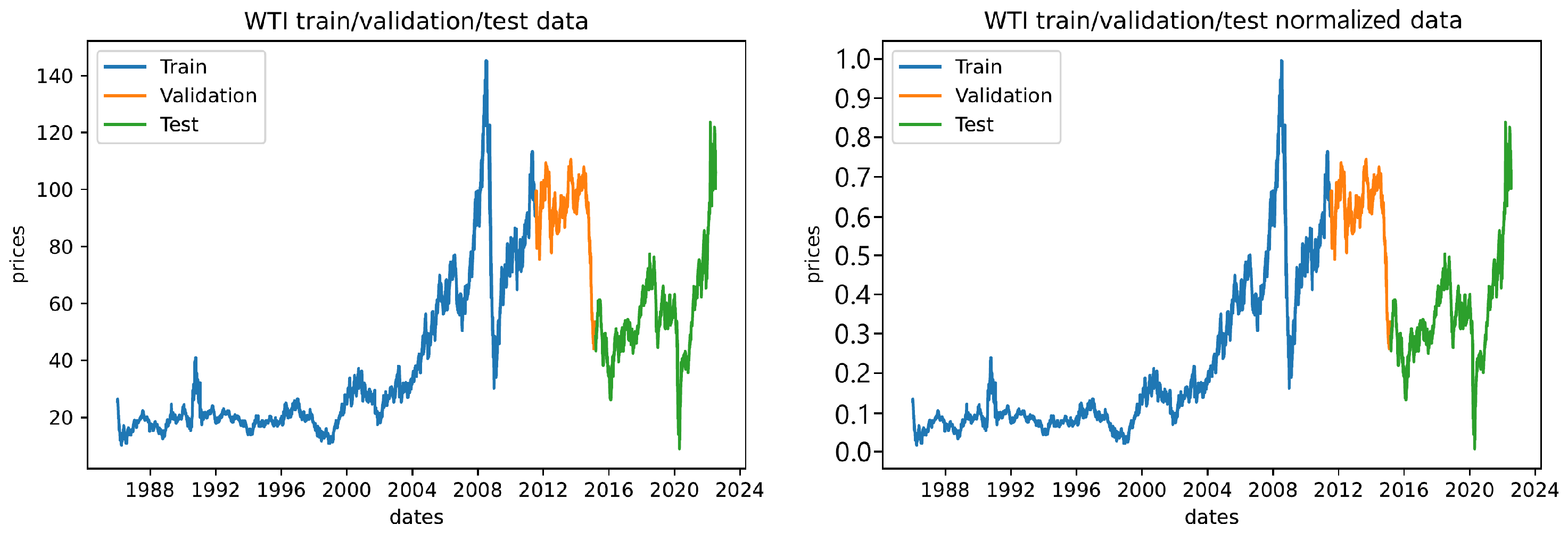
This research makes use of real-world financial data on WTI crude oil trading prices. The data encompass closing spot prices of trading days from 2 January 1986 to 11 July 2022, excluding weekends, and has been acquired from public sources provided by the United States Energy Information Administration (EIA) at https://www.eia.gov/petroleum/gasdiesel/ (accessed on 20 July 2022).

During all experimentation, the dataset has been split into training, test, and validation segments, with training being made up of the first 70% of available data, and validation of 10% subsequent data points, while the remaining 20% of data series has been used for testing, as shown in Figure 1. Furthermore, Figure 1 shows the datasets plot after applying the min-max normalization.

As already stated, the purpose of both experiments is to employ proposed SSA-DO metaheuristics to develop the best possible WTI crude oil trading prices forecasting model by tuning LSTM. Therefore, each agent for a given metaheuristic represents a set of LSTM network hyper-parameter values that are optimized. In the first experiment, every individual had 4 components ($D=4$), representing the 4 tuned LSTM hyper-parameters. A full list of optimized LSTM hyper-parameters with their respective lower and upper boundaries and data types are given in

Table 2. The LSTM hyper-parameters tuned in experiments.

Parameter	Boundaries	Data Type
number of neurons in the LSTM layer ($nn$ )	$lb=20$, $ub=200$	integer
learning rate ($lr$)	$lb=0.0001$, $ub=0.01$	double
dropout rate ($dr$)	$lb=0.001$, $ub=0.01$	double
number of training epochs ($epochs$)	$lb=100$, $ub=300$	integer

.

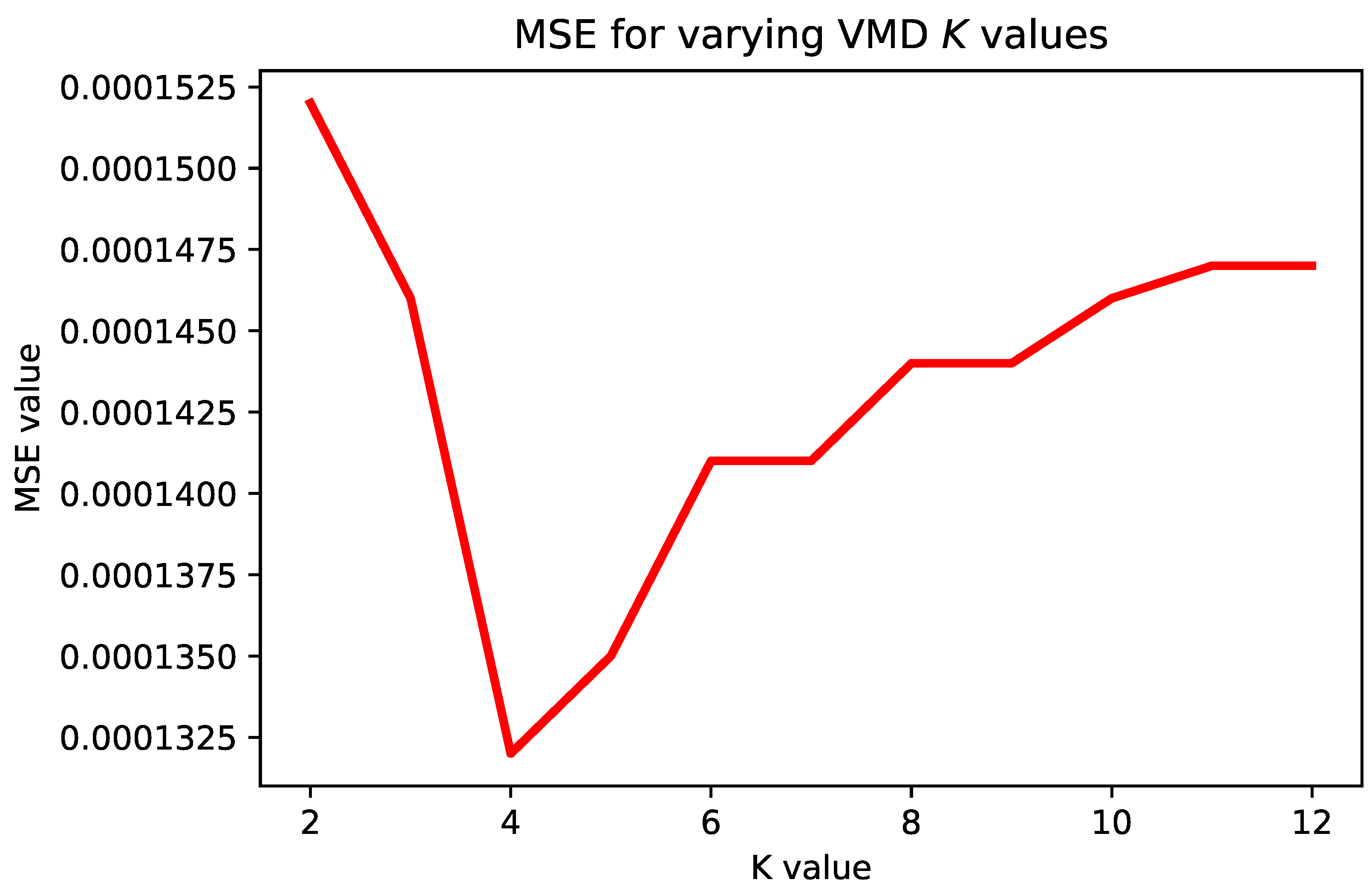
The values’ ranges for hyper-parameters have been empirically determined through extensive simulation testing using various control parameter values. For the second experiment, which incorporated VMD, the length of individuals is expended to $D=4·(K+1)$, with K representing the number of VMD signal decomposition modes. However, the decomposition process also includes a remainder (residual), hence $K+1$. The second experiment optimized the same set of hyper-parameters as the first experiment with the same ranges, however, for each time-series, including residual, generated by VMD, a separate LSTM network was developed, e.g., if K is set to 5, six LSTM structures were generated by every swarm agent.

The VMD value of parameter K has been determined empirically and it was set to 4 ($K=4$), according to extensive testing with different K values as follows: for varying K values from the range $[2, 12]$, the SSA-DO was employed for evolving LSTM structures for one step ahead simulations with 6 individuals and 5 iterations, and the mean square error (MSE) performance metric was recorded. Afterward, guided by the “elbow approach”, the K value for which the best (lowest) MSE was found is used in further experiments. Obtained results with varying K are visualized in Figure 2. It is noted that for VMD implementation, python vmd-python library was used with the following parameters: $\aleph =2000$, $\tau =0$, $DC=0$, $int=1$ and $tol=1\times {10}^{-7}$. For more details, readers can check the following URL: https://github.com/vrcarva/vmdpy (accessed on 20 July 2022).

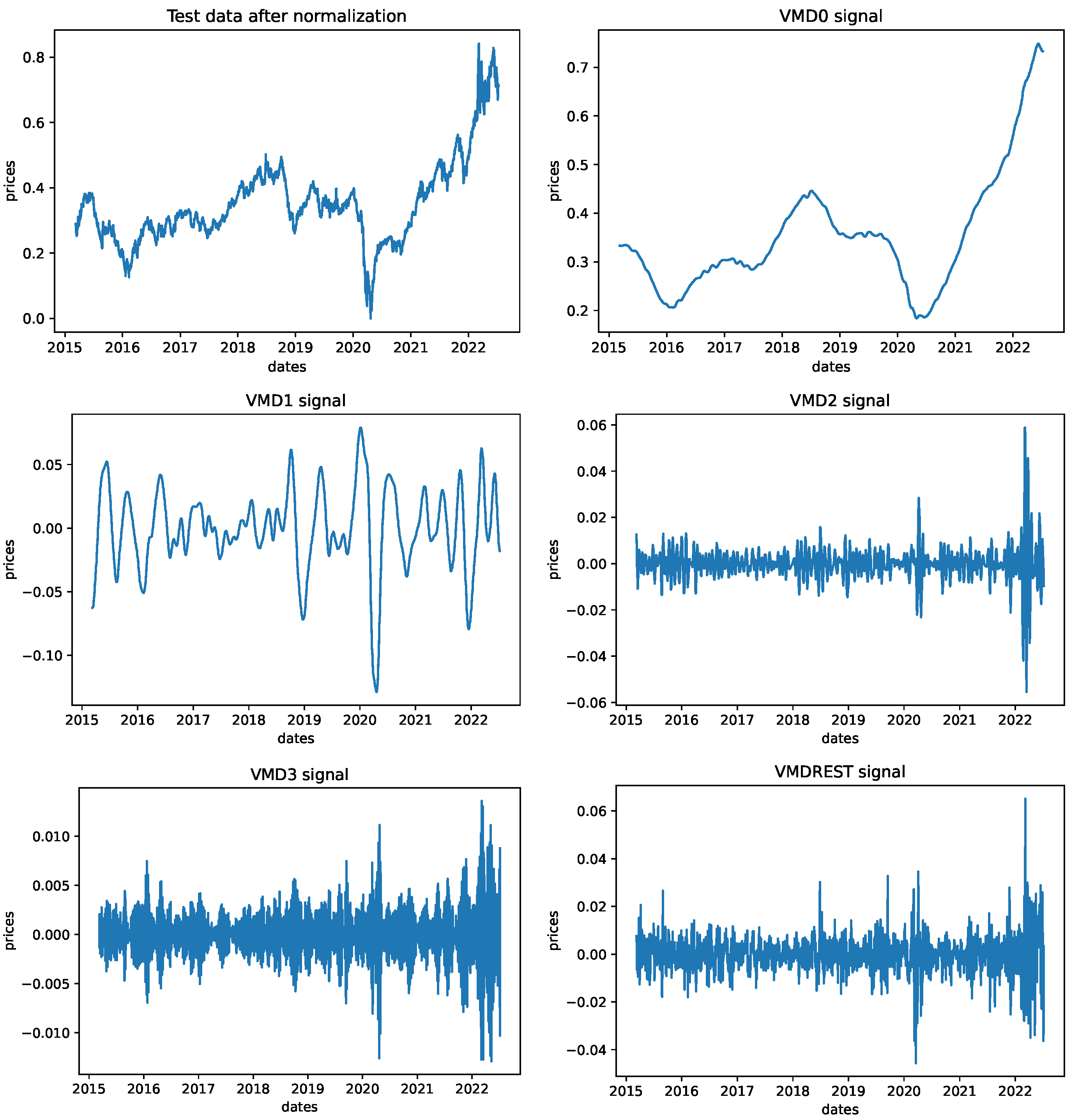
In both experiments, LSTM and VMD-LSTM, the number of LSTM neurons in the output layer is set to the number of forecasting steps ahead, where each neuron makes one prediction, e.g., for three steps ahead, there are 3 neurons in the output layer. Additionally, to improve LSTM network training, before splitting the dataset into training, testing, and validation datasets, and the normalization of all data points to the range $[0, 1]$ was performed. In the scenarios of VMD experiments, data series are decomposed after they have been normalized. At the end of the simulation, to generate graphs for the best-performing LSTM/VMD-LSTM models, all data points have been denormalized. Visual representation of the original test set data series after normalization and 4 signals along with residual generated by VMD is given in Figure 3.

The simulation framework, as well as SSA-DO and all methods used in the comparative analysis, were developed in Python using standard data science and machine learning libraries numpy, scypi, pandas, scikit-learn, tensorflow 2.0 and keras, while visualization is aided by matplotlib and seaborn.

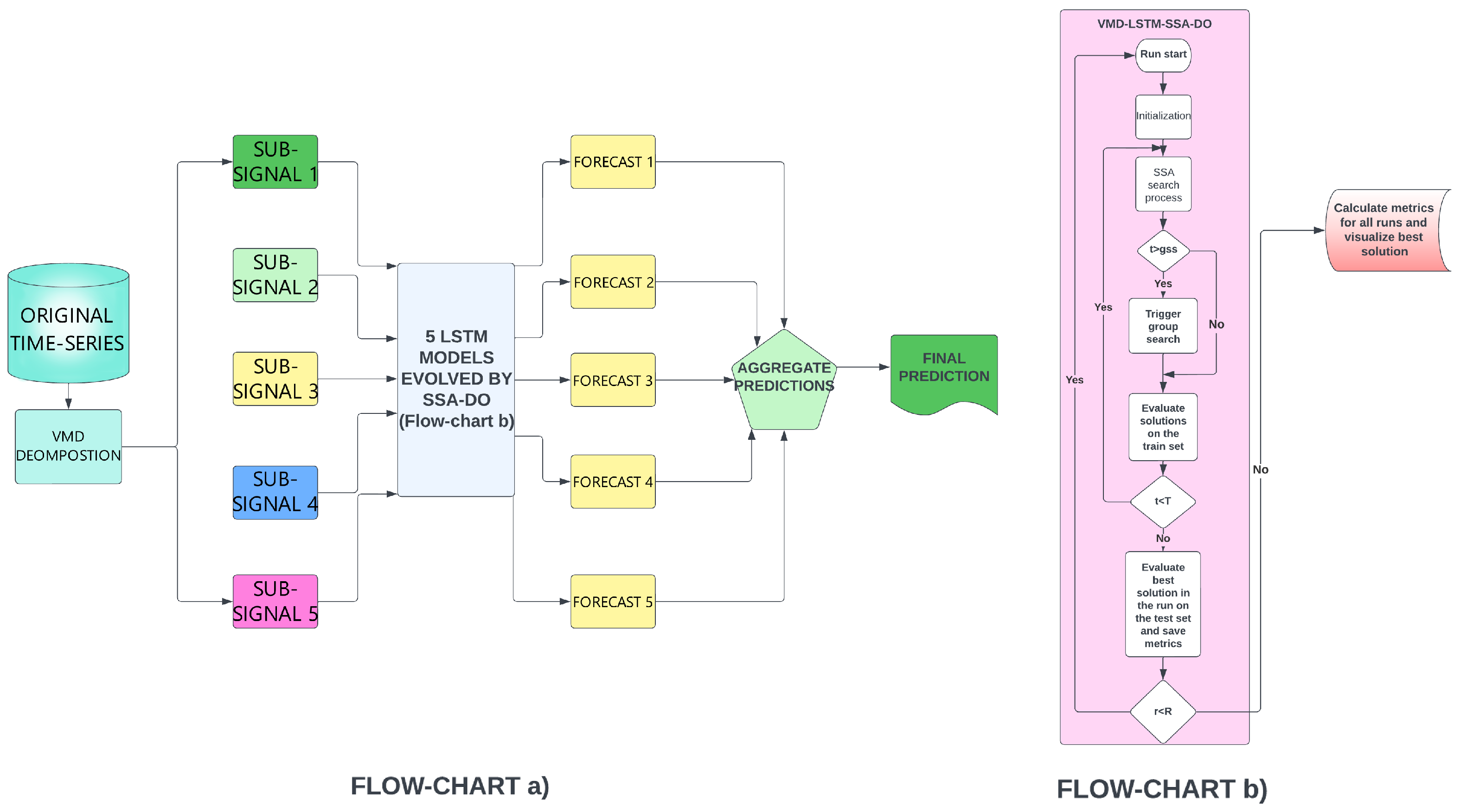
A flowchart for the developed VMD-LSTM framework is shown in Figure 4.

4.2. Evaluation Metrics, Basic Setup, and Opponent Methods

To evaluate the results of the proposed method four evaluation metrics have been used: root mean square error (RMSE), mean absolute error (MAE), mean square error (MSE), and coefficient of determination ($R^2$), calculated according to Equation (21), Equation (22), Equation (23), to Equation (24) respectively.

$$RMSE=\sqrt{\frac{1}{n}\sum _{i=1}^n{\left(y_i-\widehat{y_i}\right)}^2}$$

(21)

$$MAE=\frac{1}{n}\sum _{i=1}^n\left|y_i-\widehat{y_i}\right|$$

(22)

$$MSE=\frac{1}{n}\sum _{i=1}^n\frac{{(y_i-\widehat{y_i})}^2}{y_i}$$

(23)

$$R^2=1-\frac{{\sum }_{i=1}^n{\left(y_i-\widehat{y_i}\right)}^2}{{\sum }_{i=1}^n{\left(y_i-\overline{y}\right)}^2},$$

(24)

where $y_i$ and $\widehat{y_i}$ denote observed (real) and predicted values for i-th observation, respectively, $\overline{y}$ is arithmetic mean of real data and n is the size of the sample.

As already stated above, in one, two, and three-steps ahead experiments, generated LSTMs in the output layer have one, two, and three neurons, respectively, e.g., the LSTM for three-steps ahead, forecast for one, two, and three days are provided, one day by each neuron. Further, in all experiments (LSTM and VMD-LSTM with one, three, and five steps ahead), all indicators are determined separately, per step. However, in cases with three and five steps ahead predictions, overall metrics (oR2, oMAE, oMSE, and oRMSE) are also calculated. Such calculated overall values are not simple arithmetic means of the previous steps forecasts, e.g., overall $R2$ for a three-steps ahead experiment is not simple arithmetic mean derived from $R2$ results for one-step, two-steps and three-steps ahead, because there are some data points for which all, one, two and three-steps ahead prediction are not available. In one-step-ahead forecasting, overall and one-step-ahead metrics are the same.

To demonstrate this, let’s suppose that the first data point in the test set is 1 January 2020, the number of lags is adjusted to 3 and that three-steps ahead prediction is simulated. In this particular scenario, for the date 4 January 2022, only one result will be generated by the first neuron, which performs one-step ahead forecasting, for 5 January there will be two results, one by the first neuron and one by the second, that performs two-steps ahead forecasting. Following this pattern, the first data point for which three forecast values will be determined is 6 January 2022. The error for a particular day is the mean error of all forecasts for that day and for that reason overall metrics are not the same as the simple arithmetic mean of previous steps indicators.

The forecasting challenge is tackled as a minimization problem and the objective function is formulated with respect to the overall MSE (oMSE), as specified in the following equation:

$$Obj=min\left(oMSE\right)$$

(25)

For both experimental simulations, the tested metaheuristics were assigned a population of 6 individuals ($N=6$), that were improved over 5 iterations ($T=5$), and assessed through 6 independent runs ($R=6$). However, since the proposed SSA-DO evaluates one more candidate solution in each iteration, it was tested with only 5 individuals, and in this way, a slight advantage is given to opponent algorithms. The relatively modest population sizes, iteration, and runtime numbers are mainly due to the demanding computational nature of the experiments. Furthermore, early stopping conditions have been implemented for both experiments with $patience=\frac{epochs}{3}$, and recurrent dropout rates for the LSTM networks were kept at the default $0.01$ value along with the relu activation function, adam optimizer, mse loss function and batch size of 16.

The comparative analysis encompasses 6 state-of-the-art metaheuristics including the novel proposed SSA-DO, original SSA [4], ABC [42], FA [25], SCA [26], TLB [43], tested with default control parameters values proposed in the original works that introduced them. All algorithms were also implemented in this study and tested under the same conditions as the proposed SSA-DO.

5. Empirical Results and Analysis

This section gives an overview of experimental findings and comparative analysis with other LSTM structures generated by opponent metaheuristics and some other well-known ML models. First, findings from simulations with LSTM are given, where input is the original time-series, followed by results for generated LSTMs by using VMD decomposed inputs, afterwards comparison with other ML models for the same problem is provided and finally, to validate obtained improvements of proposed SSA-DO, rigid analysis based on conducted statistical tests is shown.

To make results more clear for presentation, metaheuristics employed in the LSTM simulations are prefixed with `LSTM’, while those utilized in experiments with VMD are prefixed with `VMD-LSTM’, e.g., LSTM-SSA-DO and VMD-LSTM-SSA-DO, respectively. It is also noted that the best results in all experimental findings tables are marked with bold style and that to fit results’ tables within the width of the page, in table headers `V-LSTM’ instead of `VMD-LSTM’ is used for denoting VMD-LSTM structures.

It is very important to note that all performance metrics provided in results tables (R2, MAE, MSE and RMSE) are shown against the normalized data points because as it was already showed in Section 4.1, to improve LSTM network training, before splitting the dataset into training, testing, and validation, and the normalization of all data points to the range $[0, 1]$ was performed. Subsequently, results for MAE, MSE, and RMSE may differ from those presented in some of the other studies [6,41], because they are represented on different scales.

5.1. Simulations with Lstm

Experimental findings and comparative analysis from experiments with LSTM without VMD are summarized in two types of tables (

Table 3. Objective function metrics over 6 runs for designed LSTM with 1 step ahead.

Method	LSTM-SSA-DO	LSTM-SSA	LSTM-ABC	LSTM-FA	LSTM-SCA	LSTM-TLB
Best	$1.45\times {10}^{-04}$	$1.72\times {10}^{-04}$	$1.61\times {10}^{-04}$	$1.48\times {10}^{-04}$	$1.58\times {10}^{-04}$	$1.48\times {10}^{-04}$
Worst	$1.78\times {10}^{-04}$	$1.86\times {10}^{-04}$	$1.66\times {10}^{-04}$	$1.99\times {10}^{-04}$	$1.73\times {10}^{-04}$	$2.01\times {10}^{-04}$
Mean	$1.58\times {10}^{-04}$	$1.77\times {10}^{-04}$	$1.63\times {10}^{-04}$	$1.69\times {10}^{-04}$	$1.61\times {10}^{-04}$	$1.64\times {10}^{-04}$
Median	$1.54\times {10}^{-04}$	$1.76\times {10}^{-04}$	$1.62\times {10}^{-04}$	$1.66\times {10}^{-04}$	$1.58\times {10}^{-04}$	$1.54\times {10}^{-04}$
Std	$1.41\times {10}^{-05}$	$6.13\times {10}^{-06}$	$2.19\times {10}^{-06}$	$2.23\times {10}^{-05}$	$6.46\times {10}^{-06}$	$2.12\times {10}^{-05}$
Var	$1.97\times {10}^{-10}$	$3.76\times {10}^{-11}$	$4.78\times {10}^{-12}$	$4.98\times {10}^{-10}$	$4.18\times {10}^{-11}$	$4.49\times {10}^{-10}$

,

Table 4. The R2, MAE, MSE, and RMSE metrics of best-generated LSTM with one step ahead.

	Indicator	LSTM-SSA-DO	LSTM-SSA	LSTM-ABC	LSTM-FA	LSTM-SCA	LSTM-TLB
One-step ahead	R2	0.991122	0.989395	0.989919	0.990655	0.990050	0.990848
	MAE	0.008316	0.009039	0.008800	0.008401	0.008679	0.008510
	MSE	0.000145	0.000172	0.000161	0.000148	0.000158	0.000148
	RMSE	0.012038	0.013097	0.012694	0.012158	0.012557	0.012152
Overall Results	oR2	0.991122	0.989395	0.989919	0.990655	0.990050	0.990848
	oMAE	0.008316	0.009039	0.008800	0.008401	0.008679	0.008510
	oMSE	0.000145	0.000172	0.000161	0.000148	0.000158	0.000148
	oRMSE	0.012038	0.013097	0.012694	0.012158	0.012557	0.012152

,

Table 5. Objective function metrics over 6 runs for designed LSTM with 3 steps ahead.

Method	LSTM-SSA-DO	LSTM-SSA	LSTM-ABC	LSTM-FA	LSTM-SCA	LSTM-TLB
Best	$1.50\times {10}^{-04}$	$1.51\times {10}^{-04}$	$1.57\times {10}^{-04}$	$1.57\times {10}^{-04}$	$1.52\times {10}^{-04}$	$1.57\times {10}^{-04}$
Worst	$1.50\times {10}^{-04}$	$1.84\times {10}^{-04}$	$1.76\times {10}^{-04}$	$1.71\times {10}^{-04}$	$1.68\times {10}^{-04}$	$1.74\times {10}^{-04}$
Mean	$1.50\times {10}^{-04}$	$1.69\times {10}^{-04}$	$1.66\times {10}^{-04}$	$1.62\times {10}^{-04}$	$1.56\times {10}^{-04}$	$1.62\times {10}^{-04}$
Median	$1.50\times {10}^{-04}$	$1.70\times {10}^{-04}$	$1.66\times {10}^{-04}$	$1.59\times {10}^{-04}$	$1.52\times {10}^{-04}$	$1.57\times {10}^{-04}$
Std	$0.00\times {10}^{+00}$	$1.39\times {10}^{-05}$	$7.39\times {10}^{-06}$	$5.70\times {10}^{-06}$	$7.30\times {10}^{-06}$	$7.07\times {10}^{-06}$
Var	$0.00\times {10}^{+00}$	$1.93\times {10}^{-10}$	$5.46\times {10}^{-11}$	$3.25\times {10}^{-11}$	$5.34\times {10}^{-11}$	$5.00\times {10}^{-11}$

,

Table 6. The R2, MAE, MSE, and RMSE metrics of best-generated LSTM with three steps ahead.

	Indicator	LSTM-SSA-DO	LSTM-SSA	LSTM-ABC	LSTM-FA	LSTM-SCA	LSTM-TLB
One-step ahead	R2	0.990881	0.991324	0.990710	0.990619	0.989925	0.990662
	MAE	0.008325	0.008164	0.008391	0.008493	0.008783	0.008455
	MSE	0.000145	0.000137	0.000145	0.000149	0.000156	0.000148
	RMSE	0.012062	0.011720	0.012059	0.012218	0.012494	0.012159
Two-step ahead	R2	0.990158	0.989644	0.989138	0.988947	0.990454	0.989714
	MAE	0.008578	0.008989	0.009008	0.009072	0.008620	0.008746
	MSE	0.000157	0.000161	0.000174	0.000170	0.000148	0.000164
	RMSE	0.012526	0.012672	0.013198	0.013022	0.012152	0.012799
Three-step ahead	R2	0.990903	0.989947	0.990121	0.990429	0.990583	0.989611
	MAE	0.008521	0.008925	0.008911	0.008471	0.008486	0.008961
	MSE	0.000148	0.000156	0.000151	0.000151	0.000151	0.000161
	RMSE	0.012163	0.012500	0.012308	0.012303	0.012284	0.012680
Overall Results	oR2	0.990651	0.990312	0.989983	0.990013	0.990326	0.989999
	oMAE	0.008475	0.008693	0.008770	0.008679	0.008630	0.008721
	oMSE	0.000150	0.000151	0.000157	0.000157	0.000152	0.000157
	oRMSE	0.012252	0.012304	0.012531	0.012520	0.012311	0.012549

,

Table 7. Objective function metrics over 6 runs for designed LSTM with 5 steps ahead.

Method	LSTM-SSA-DO	LSTM-SSA	LSTM-ABC	LSTM-FA	LSTM-SCA	LSTM-TLB
Best	$1.58\times {10}^{-04}$	$1.47\times {10}^{-04}$	$1.56\times {10}^{-04}$	$1.58\times {10}^{-04}$	$1.56\times {10}^{-04}$	$1.67\times {10}^{-04}$
Worst	$1.61\times {10}^{-04}$	$1.72\times {10}^{-04}$	$1.70\times {10}^{-04}$	$1.64\times {10}^{-04}$	$1.84\times {10}^{-04}$	$1.71\times {10}^{-04}$
Mean	$1.58\times {10}^{-04}$	$1.53\times {10}^{-04}$	$1.65\times {10}^{-04}$	$1.63\times {10}^{-04}$	$1.71\times {10}^{-04}$	$1.69\times {10}^{-04}$
Median	$1.58\times {10}^{-04}$	$1.47\times {10}^{-04}$	$1.66\times {10}^{-04}$	$1.64\times {10}^{-04}$	$1.73\times {10}^{-04}$	$1.68\times {10}^{-04}$
Std	$1.35\times {10}^{-06}$	$1.11\times {10}^{-05}$	$5.95\times {10}^{-06}$	$2.82\times {10}^{-06}$	$9.97\times {10}^{-06}$	$1.47\times {10}^{-06}$
Var	$1.83\times {10}^{-12}$	$1.23\times {10}^{-10}$	$3.54\times {10}^{-11}$	$7.95\times {10}^{-12}$	$9.95\times {10}^{-11}$	$2.17\times {10}^{-12}$

and

Table 8. The R2, MAE, MSE, and RMSE metrics of best-generated LSTM with five steps ahead.

	Indicator	LSTM-SSA-DO	LSTM-SSA	LSTM-ABC	LSTM-FA	LSTM-SCA	LSTM-TLB
One-step ahead	R2	0.991234	0.988886	0.988907	0.990731	0.990851	0.989556
	MAE	0.008247	0.009384	0.009398	0.008434	0.008366	0.008730
	oMSE	0.000138	0.000173	0.000170	0.000143	0.000144	0.000164
	RMSE	0.011742	0.013146	0.013036	0.011957	0.012006	0.012805
Two-step ahead	R2	0.989951	0.989009	0.990213	0.989825	0.990641	0.990652
	MAE	0.008755	0.009253	0.008787	0.008802	0.008733	0.008269
	MSE	0.000156	0.000171	0.000151	0.000157	0.000143	0.000146
	RMSE	0.012506	0.013065	0.012276	0.012523	0.011956	0.012096
Three-step ahead	R2	0.990582	0.993458	0.989895	0.989672	0.988061	0.988564
	MAE	0.008447	0.007005	0.008764	0.008770	0.010019	0.009146
	MSE	0.000149	0.000103	0.000155	0.000161	0.000184	0.000177
	RMSE	0.012206	0.010135	0.012466	0.012689	0.013568	0.013306
Four-step ahead	R2	0.988928	0.990105	0.990078	0.990676	0.990390	0.988959
	MAE	0.009338	0.008923	0.008712	0.008357	0.008551	0.009067
	MSE	0.000173	0.000153	0.000153	0.000144	0.000150	0.000171
	RMSE	0.013153	0.012375	0.012352	0.012002	0.012238	0.013082
Five-step ahead	R2	0.988980	0.991353	0.989974	0.987868	0.989727	0.988580
	MAE	0.009278	0.008239	0.008957	0.009910	0.009086	0.009205
	MSE	0.000171	0.000133	0.000153	0.000184	0.000160	0.000177
	RMSE	0.013086	0.011546	0.012379	0.013580	0.012636	0.013297
Overall Results	oR2	0.989940	0.990568	0.989814	0.989761	0.989938	0.989266
	oMAE	0.008813	0.008561	0.008924	0.008855	0.008951	0.008883
	oMSE	0.000158	0.000147	0.000156	0.000158	0.000156	0.000167
	oRMSE	0.012550	0.012105	0.012505	0.012564	0.012495	0.012925

). First, best, worst, mean, median, standard deviation, and variance of the objective function ($oMSE$) over 10 independent runs are shown in Table 3, Table 5 and Table 7 for one, three, and five steps ahead, respectively.

In the second types of tables, R2, MAE, MSE and RMSE performance indicators for the objective obtained in the best run, are shown for each step separately along with its overall values. These results are presented in Table 4, Table 6 and Table 8 for one, three, and five steps ahead simulations, respectively. The best result in each category is noted in bold style.

All experimental findings clearly indicate that on average, SSA-DO generates the best results. In the one-step-ahead simulation, LSTM-SSA-DO managed to obtain the best result, but also the best stability, which can be perceived from the mean objective value over 6 runs. However, in this type of simulation, the LSTM-ABC achieves the best standard deviation and variance. Additionally, from Table 4 can be undoubtedly concluded that the LSTM-SSA-DO established the best performance when all metrics are considered.

In three-steps ahead experiments, LSTM-SSA-DO manifests the best stability, as well as performance, which can be seen from Table 5. Surprisingly, in all 6 runs, the LSTM-SSA-DO managed to establish the same value for the objective with zero std and variance, which at the same time achieved the best result among all metaheuristics. In this type of experiment, the second best LSTM-SSA, therefore it can be concluded that the SSA also performed well in this test.

Finally, in the five-steps-ahead experiment (Table 7 and Table 8), proposed LSTM-SSA-DO established the best stability with the lowest std and variance values, however, the best performing metaheuristics is LSTM-SSA. Therefore, the no free lunch (NFL) theorem, which states that the universally best method for all types of challenges does not exist, proved right in LSTM simulations.

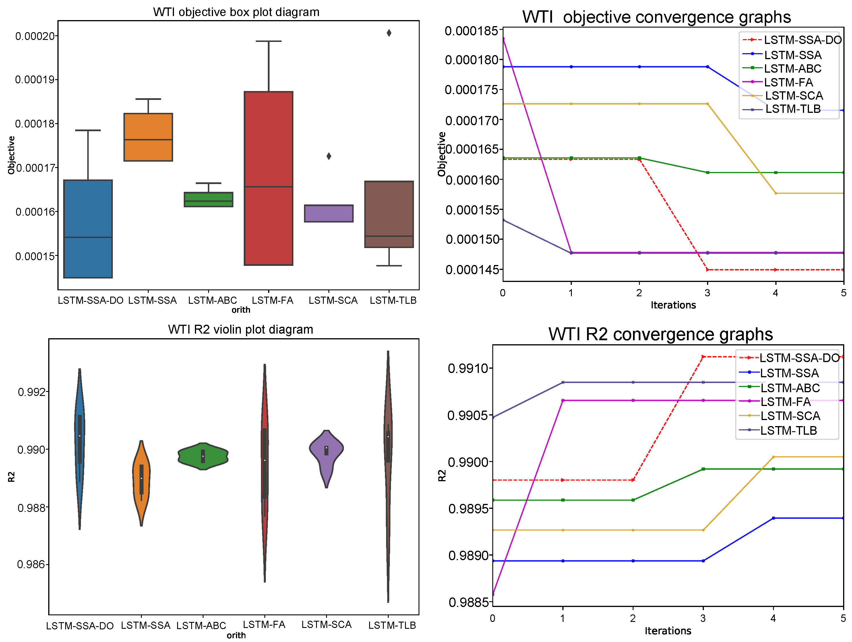
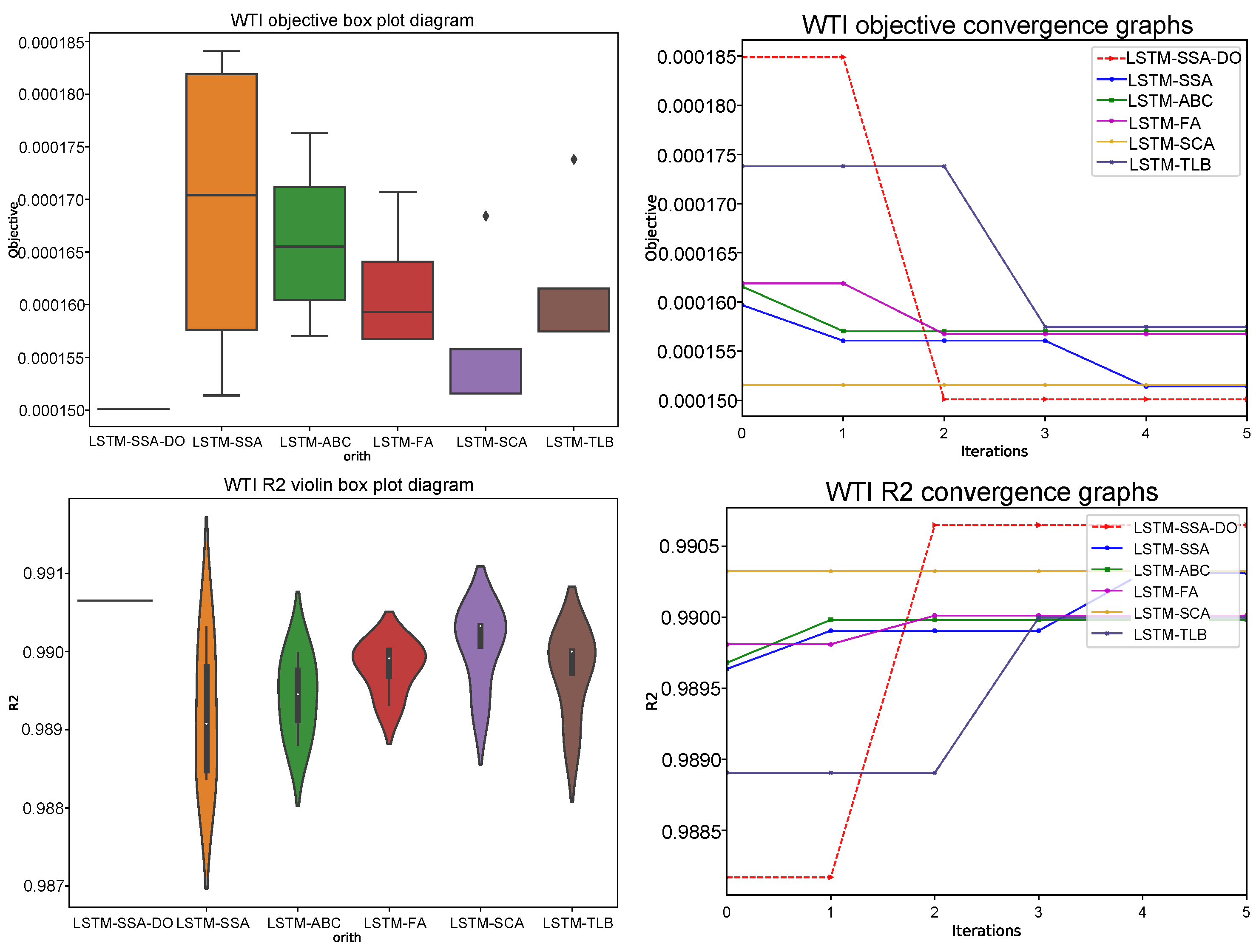
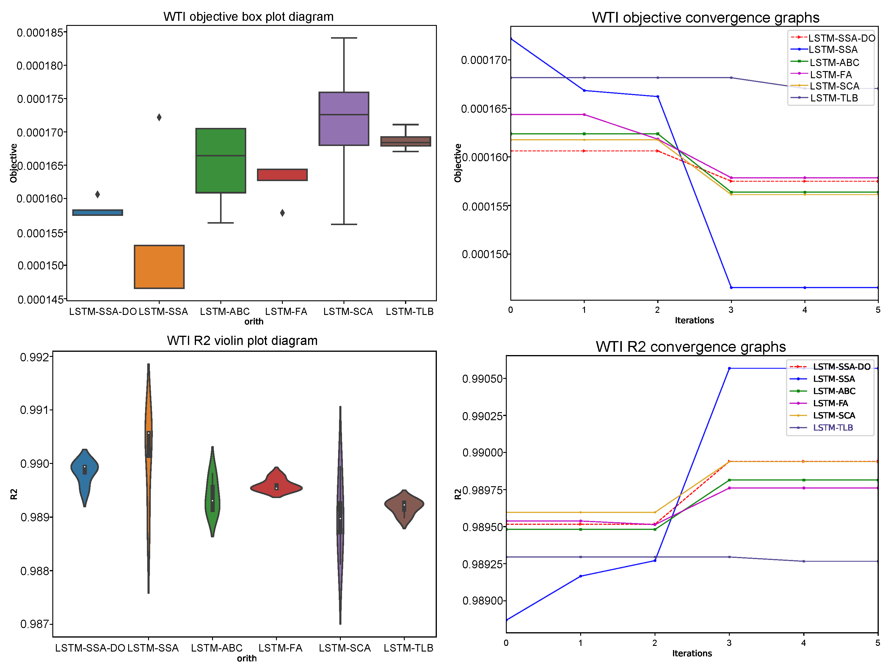
Comparative analysis visualization for LSTM experiments is provided in Figure 5, Figure 6 and Figure 7 with one, three, and five steps ahead, respectively. All provided figures include the following diagrams: box and whiskers for the objective function and violin plots for R2 indicator over 6 runs, convergence speed graphs for the objective function, and R2 metrics in the best run over 5 iterations.

From the presented diagrams it is interesting to visually compare the LSTM-SSA-DO convergence speed with other metaheuristics convergence, where can be seen that the LSTM-SSA-DO rapidly converges after $T/3$ iterations when the group search mode is triggered. Unfortunately, due to the computing resources requirements, all testing was performed with only 5 iterations, however from the statistical point of view, if more iterations were utilized the LSTM-SSA-DO would also probably be in the five-steps ahead simulation to achieve the best results.

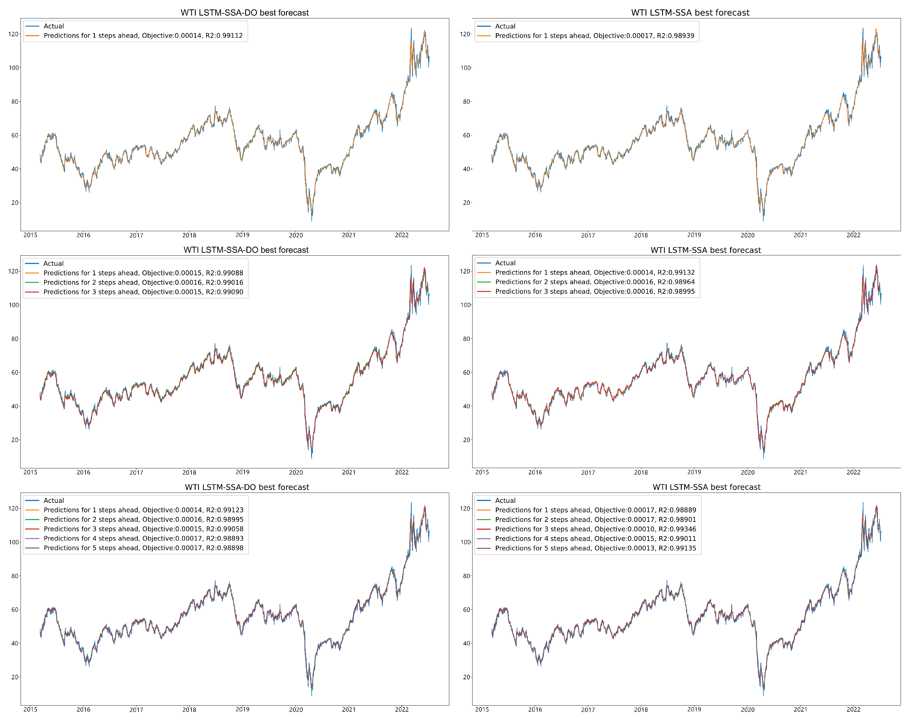
Finally, the forecast and actual results for LSTM-SSA-DO and LSTM-SSA for all LSTM simulations of the best run are depicted in Figure 8.

5.2. Simulations with VMD-LSTM

Similarly as in experiments without VMD (Section 5.1), generated results by LSTM structures that use VMD decomposed series as input, are grouped into two types of tables (

Table 9. Objective function metrics over 6 runs for designed LSTM with VMD decomposition and 1 step ahead.

Method	V-LSTM-SSA-DO	V-LSTM-SSA	V-LSTM-ABC	V-LSTM-FA	V-LSTM-SCA	V-LSTM-TLB
Best	$1.20\times {10}^{-04}$	$1.36\times {10}^{-04}$	$1.62\times {10}^{-04}$	$1.28\times {10}^{-04}$	$1.24\times {10}^{-04}$	$1.23\times {10}^{-04}$
Worst	$1.31\times {10}^{-04}$	$1.79\times {10}^{-04}$	$1.92\times {10}^{-04}$	$1.40\times {10}^{-04}$	$1.33\times {10}^{-04}$	$1.81\times {10}^{-04}$
Mean	$1.24\times {10}^{-04}$	$1.53\times {10}^{-04}$	$1.70\times {10}^{-04}$	$1.36\times {10}^{-04}$	$1.26\times {10}^{-04}$	$1.44\times {10}^{-04}$
Median	$1.23\times {10}^{-04}$	$1.49\times {10}^{-04}$	$1.62\times {10}^{-04}$	$1.37\times {10}^{-04}$	$1.24\times {10}^{-04}$	$1.35\times {10}^{-04}$
Std	$4.91\times {10}^{-06}$	$1.86\times {10}^{-05}$	$1.27\times {10}^{-05}$	$4.43\times {10}^{-06}$	$3.93\times {10}^{-06}$	$2.37\times {10}^{-05}$
Var	$1.76\times {10}^{-11}$	$3.46\times {10}^{-10}$	$1.62\times {10}^{-10}$	$1.96\times {10}^{-11}$	$1.55\times {10}^{-11}$	$5.63\times {10}^{-10}$

,

Table 10. The R2, MAE, MSE, and RMSE metrics of best-generated LSTM with VMD decomposition and 1 step ahead.

	Indicator	V-LSTM-SSA-DO	V-LSTM-SSA	V-LSTM-ABC	V-LSTM-FA	V-LSTM-SCA	V-LSTM-TLB
One-step ahead	R2	0.992600	0.991702	0.989792	0.992217	0.992354	0.992422
	MAE	0.007519	0.008144	0.009036	0.007870	0.007608	0.007766
	MSE	0.000120	0.000136	0.000162	0.000128	0.000124	0.000123
	RMSE	0.010962	0.011648	0.012724	0.011334	0.011136	0.011103
Overall Results	oR2	0.992600	0.991702	0.989792	0.992217	0.992354	0.992422
	oMAE	0.007519	0.008144	0.009036	0.007870	0.007608	0.007766
	oMSE	0.000120	0.000136	0.000162	0.000128	0.000124	0.000123
	oRMSE	0.010962	0.011648	0.012724	0.011334	0.011136	0.011103

,

Table 11. Objective function metrics over 6 runs for designed LSTM with VMD decomposition and 3 steps ahead.

Method	V-LSTM-SSA-DO	V-LSTM-SSA	V-LSTM-ABC	V-LSTM-FA	V-LSTM-SCA	V-LSTM-TLB
Best	$1.18\times {10}^{-04}$	$1.43\times {10}^{-04}$	$1.29\times {10}^{-04}$	$1.26\times {10}^{-04}$	$1.30\times {10}^{-04}$	$1.29\times {10}^{-04}$
Worst	$1.18\times {10}^{-04}$	$1.61\times {10}^{-04}$	$1.35\times {10}^{-04}$	$1.61\times {10}^{-04}$	$1.30\times {10}^{-04}$	$1.61\times {10}^{-04}$
Mean	$1.18\times {10}^{-04}$	$1.49\times {10}^{-04}$	$1.31\times {10}^{-04}$	$1.46\times {10}^{-04}$	$1.30\times {10}^{-04}$	$1.37\times {10}^{-04}$
Median	$1.18\times {10}^{-04}$	$1.46\times {10}^{-04}$	$1.30\times {10}^{-04}$	$1.48\times {10}^{-04}$	$1.30\times {10}^{-04}$	$1.29\times {10}^{-04}$
Std	$0.00\times {10}^{+00}$	$7.09\times {10}^{-06}$	$2.29\times {10}^{-06}$	$1.27\times {10}^{-05}$	$0.00\times {10}^{+00}$	$1.41\times {10}^{-05}$
Var	$0.00\times {10}^{+00}$	$5.02\times {10}^{-11}$	$5.26\times {10}^{-12}$	$1.63\times {10}^{-10}$	$0.00\times {10}^{+00}$	$2.00\times {10}^{-10}$

,

Table 12. The R2, MAE, MSE, and RMSE metrics of best-generated LSTM with VMD decomposition and 3 steps ahead.

	Indicator	V-LSTM-SSA-DO	V-LSTM-SSA	V-LSTM-ABC	V-LSTM-FA	V-LSTM-SCA	V-LSTM-TLB
One-step ahead	R2	0.992316	0.990960	0.991950	0.992286	0.991962	0.990795
	MAE	0.007965	0.008323	0.007904	0.007755	0.008046	0.008582
	MSE	0.000122	0.000143	0.000126	0.000124	0.000126	0.000141
	RMSE	0.011052	0.011946	0.011230	0.011151	0.011224	0.011892
Two-step ahead	R2	0.992632	0.990838	0.991967	0.992407	0.991823	0.992146
	MAE	0.007640	0.008418	0.008066	0.007694	0.008478	0.007654
	MSE	0.000118	0.000145	0.000126	0.000121	0.000126	0.000124
	RMSE	0.010881	0.012042	0.011215	0.011012	0.011235	0.011125
Three-step ahead	R2	0.993055	0.991025	0.991179	0.991624	0.991165	0.992224
	MAE	0.007329	0.008316	0.008829	0.008335	0.008425	0.007727
	MSE	0.000113	0.000143	0.000136	0.000132	0.000139	0.000121
	RMSE	0.010610	0.011943	0.011657	0.011480	0.011780	0.010998
Overall Results	oR2	0.992671	0.990941	0.991702	0.992110	0.991649	0.991728
	oMAE	0.007645	0.008353	0.008266	0.007928	0.008316	0.007988
	oMSE	0.000118	0.000143	0.000129	0.000126	0.000130	0.000129
	oRMSE	0.010849	0.011977	0.011369	0.011216	0.011416	0.011345

,

Table 13. Objective function metrics over 6 runs for designed LSTM with VMD decomposition and 5 steps ahead.

Method	V-LSTM-SSA-DO	V-LSTM-SSA	V-LSTM-ABC	V-LSTM-FA	V-LSTM-SCA	V-LSTM-TLB
Best	$1.23\times {10}^{-04}$	$1.24\times {10}^{-04}$	$1.35\times {10}^{-04}$	$1.45\times {10}^{-04}$	$1.30\times {10}^{-04}$	$1.44\times {10}^{-04}$
Worst	$1.53\times {10}^{-04}$	$1.52\times {10}^{-04}$	$1.53\times {10}^{-04}$	$1.72\times {10}^{-04}$	$1.32\times {10}^{-04}$	$1.53\times {10}^{-04}$
Mean	$1.31\times {10}^{-04}$	$1.31\times {10}^{-04}$	$1.44\times {10}^{-04}$	$1.52\times {10}^{-04}$	$1.31\times {10}^{-04}$	$1.48\times {10}^{-04}$
Median	$1.37\times {10}^{-04}$	$1.24\times {10}^{-04}$	$1.44\times {10}^{-04}$	$1.47\times {10}^{-04}$	$1.31\times {10}^{-04}$	$1.48\times {10}^{-04}$
Std	$1.20\times {10}^{-05}$	$1.21\times {10}^{-05}$	$9.12\times {10}^{-06}$	$1.11\times {10}^{-05}$	$1.07\times {10}^{-06}$	$3.28\times {10}^{-06}$
Var	$1.44\times {10}^{-10}$	$1.46\times {10}^{-10}$	$8.31\times {10}^{-11}$	$1.23\times {10}^{-10}$	$1.14\times {10}^{-12}$	$1.08\times {10}^{-11}$

and

Table 14. The R2, MAE, MSE, and RMSE metrics of best-generated LSTM with VMD decomposition and 5 steps ahead.

	Indicator	V-LSTM-SSA-DO	V-LSTM-SSA	V-LSTM-ABC	V-LSTM-FA	V-LSTM-SCA	V-LSTM-TLB
One-step ahead	R2	0.992395	0.992102	0.991933	0.991107	0.990937	0.990601
	MAE	0.007887	0.008103	0.007852	0.008185	0.008494	0.008341
	MSE	0.000120	0.000124	0.000126	0.000138	0.000139	0.000147
	RMSE	0.010951	0.011136	0.011240	0.011767	0.011787	0.012106
Two-step ahead	R2	0.991830	0.992238	0.991093	0.990885	0.990924	0.991174
	MAE	0.007919	0.007780	0.008225	0.008211	0.008366	0.008093
	MSE	0.000128	0.000122	0.000140	0.000146	0.000140	0.000139
	RMSE	0.011310	0.011031	0.011825	0.012091	0.011824	0.011773
Three-step ahead	R2	0.992849	0.991362	0.990792	0.991338	0.991388	0.990492
	MAE	0.007451	0.008431	0.008517	0.007958	0.008170	0.008413
	MSE	0.000112	0.000135	0.000142	0.000134	0.000133	0.000151
	RMSE	0.010592	0.011631	0.011925	0.011574	0.011513	0.012296
Four-step ahead	R2	0.991402	0.992149	0.992103	0.991214	0.992857	0.991043
	MAE	0.008111	0.008038	0.007781	0.008107	0.007357	0.008219
	MSE	0.000141	0.000122	0.000123	0.000135	0.000111	0.000140
	RMSE	0.011866	0.011030	0.011080	0.011626	0.010529	0.011815
Five-step ahead	R2	0.992801	0.992615	0.990827	0.988709	0.991850	0.990621
	MAE	0.007478	0.007596	0.008513	0.009749	0.007999	0.008355
	MSE	0.000113	0.000116	0.000142	0.000170	0.000125	0.000145
	RMSE	0.010644	0.010757	0.011913	0.013025	0.011202	0.012033
Overall Results	oR2	0.992250	0.992093	0.991352	0.990666	0.991594	0.990786
	oMAE	0.007769	0.007989	0.008178	0.008442	0.008077	0.008284
	oMSE	0.000123	0.000124	0.000135	0.000145	0.000130	0.000144
	oRMSE	0.011082	0.011121	0.011602	0.012028	0.011381	0.012006

). Comparative analysis between proposed VMD-LSTM-SSA-DO and other methods of best, worst, mean, median, standard deviation, and variance of the objective function ($oMSE$) over six runs is presented for one, three, and five steps ahead in Table 9, Table 11 and Table 13, respectively. On the other side, R2, MAE, MSE and RMSE indicators for the best objective per each step, as well its overall values, are shown in Table 10, Table 12 and Table 14 for one, three, and five steps ahead simulations, respectively.

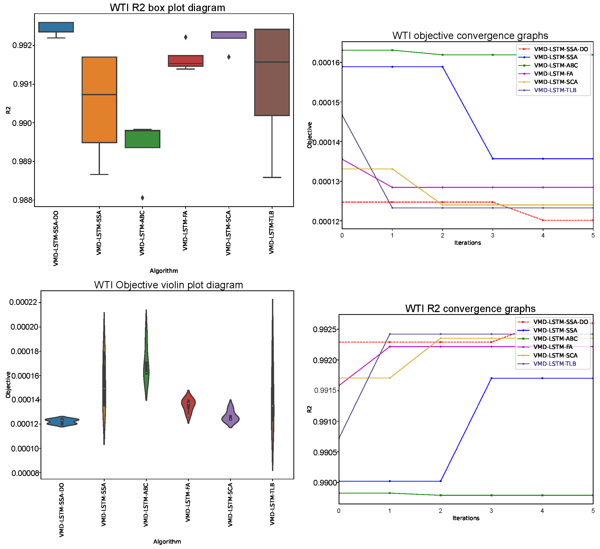
Again, as in the previous experiment, the VMD-LSTM-SSA-DO on average showed the best performance among all competitor algorithms. However, the NFL theorem has also been validated in this experiment, and the VMD-LSTM-SSA-DO was outscored by other approaches in some cases. It also should be noted that in all cases, VMD-LSTM-SSA-DO proved to be more robust than its baseline method, VMD-LSTM-SSA.

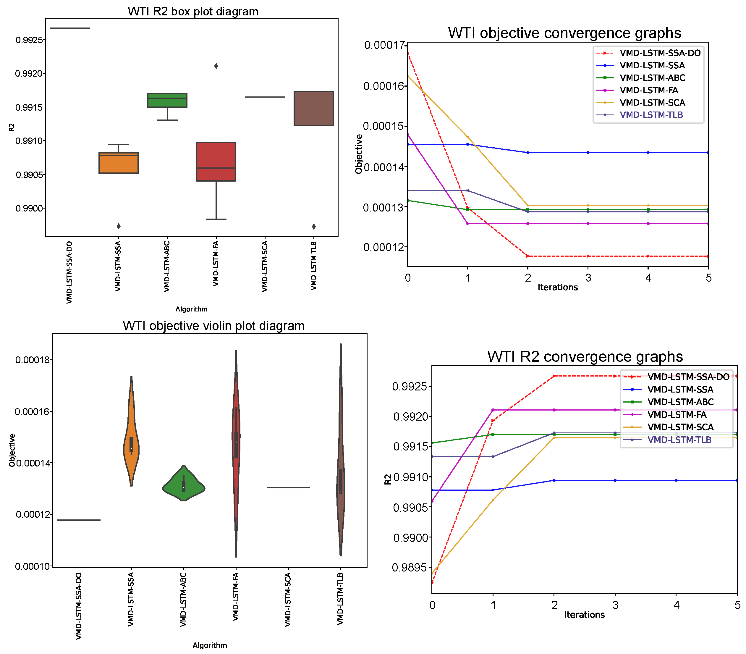
From results tables with one-step ahead (Table 9 and Table 10), can be observed that the introduced VMD-LSTM-SSA-DO managed to obtain the best value for $oMSE$, outscoring the second best approach, VMD-LSTM-SCA, by $4.00\times {10}^{-05}$. Moreover, the VMD-LSTM-SSA-DO proved to be the most stable approach among all metaheuristics, obtaining the best values also for worst, mean and median metrics. The VMD-LSTM-SCA outscored VMD-LSTM-SSA-DO only in standard deviation and variance comparisons. Detailed metrics of the best run, presented in Table 10 clearly indicate the superiority of VMD-LSTM-SSA-DO over others.

Interestingly, in three-steps ahead simulation (Table 11 and Table 12), like in the previous experiment for the same number of steps ahead, VMD-LSTM-SSA-DO showed the best stability along with the VMD-LSTM-SCA. Both methods in each run generated LSTM structures with the same performance. However, the accuracy of LSTMs obtained by VMD-LSTM-SSA-DO is substantially better than the ones generated by the VMD-LSTM-SCA. Additionally, in this simulation, VMD-LSTM-SSA-DO solutions’ quality is much better than all other metaheuristics.

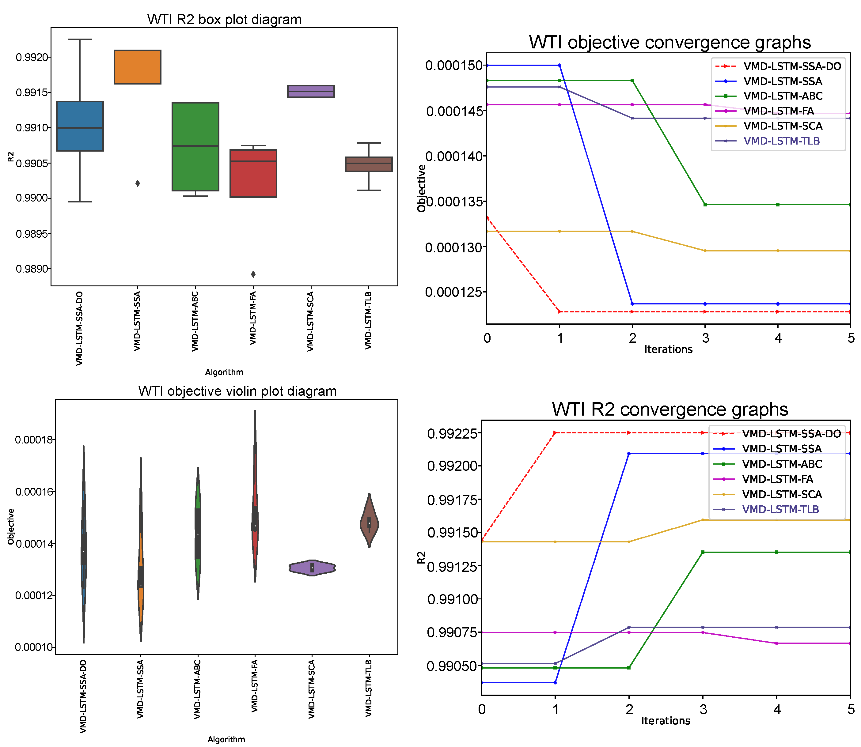
Finally, in five-steps ahead simulation (Table 13 and Table 14), VMD-LSTM-SSA-DO showed the best ability to find the best performing LSTM structures, outscoring the second-best approach, VMD-LSTM-SSA, as well as all other methods included in analysis. Additionally, the VMD-LSTM-SSA-DO obtained the best mean values along with the VMD-LSTM-SSA and VMD-LSTM-SCA. It is interesting to notice that in this experiment, the original SSA showed better accomplishments than other opponent methods excluding SSA-DO.

Figure 9, Figure 10 and Figure 11 show a visual representation of three conducted VMD-LSTM simulations, where violin plots for objective and box plots for R2 indicator over 6 runs along with convergence speed graphs for objective and R2 in the best run, are presented.

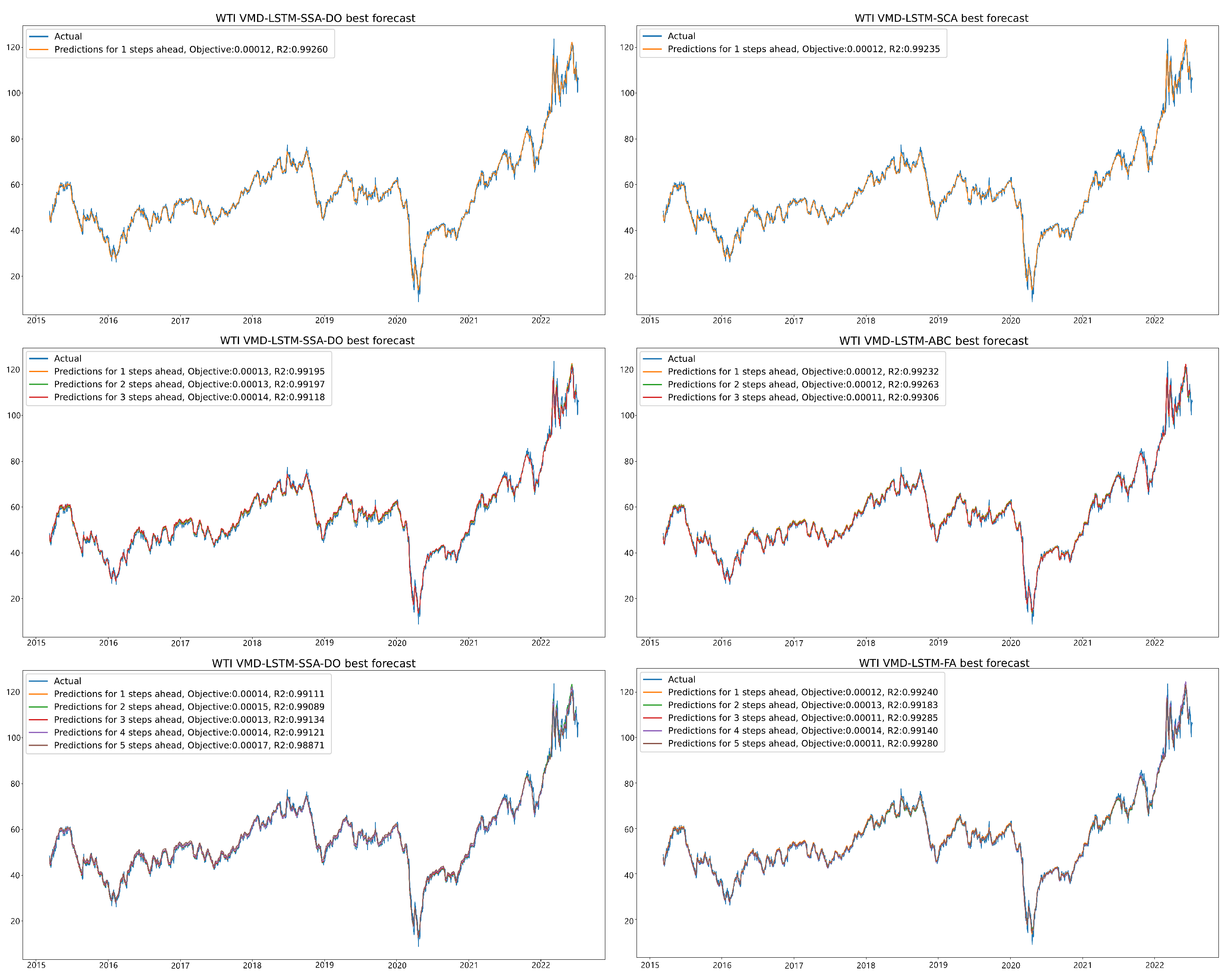
Visual comparison between predicted and actual time-series values for VMD-LSTM-SSA-DO and some of the chosen other methods for one-step, three-steps, and five-steps ahead simulations is provided in Figure 12.

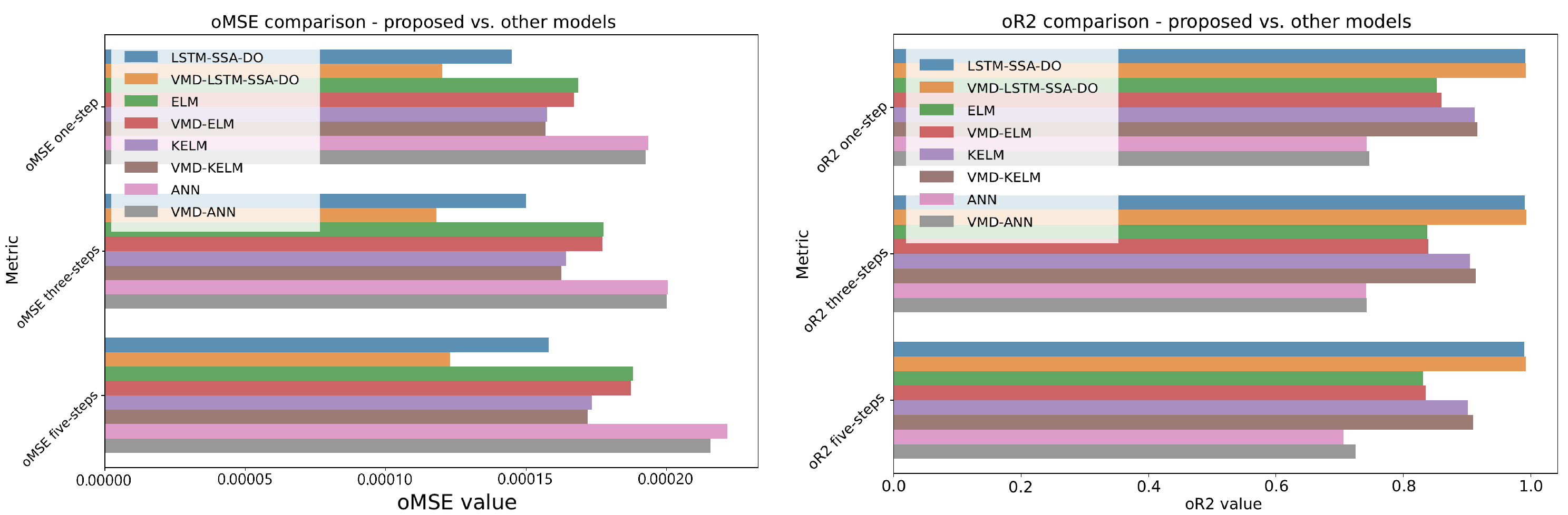
5.3. Comparison with Other Well-Known Methods

With the goal of wider comparative analysis, developed LSTM-SSA-DO and VMD-LSTM-SSA-DO models are compared with some approaches presented in [6,41]. In additional experiments, extreme learning machine (ELM), kernel ELM (KELM), and simple ANN with one hidden layer with and without VMD were also implemented and tested for one, three and five-steps prediction under the same experimental conditions, described in Section 4.

Supplementary models were not tuned by metaheuristics, instead, a simple manual grid search was performed and the results of best performing models were reported. The following hyper-parameters were investigated: for all three models the number of neurons in the hidden layer within the boundaries $[20, 200]$ with a step of 10, for ANN the number of training epochs and dropout rate within the boundaries $[100, 300]$ with step 20 and $[0.001, 0.01]$ with step 0.02, respectively, and for the KELM, the regularization parameter C withing the range $[10, 100]$ with step 10 and kernel bandwidth $\sigma$ within the interval $[0, 1]$ with step 0.1. The ANN was validated against the validation data, and the $epochs/3$ was set as an early stopping condition, the same as in the LSTM simulations.

Comparative analysis of obtained oMSE and oR2 indicators is provided in

Table 15. Comparison with standard ML models.

Model	oMSE 1-Step	oMSE 3-Steps	oMSE 5-Steps	oR2 1-Step	oR2 3-Steps	oR2 5-Steps
LSTM-SSA-DO	0.000145	0.000150	0.000158	0.991122	0.990651	0.989940
VMD-LSTM-SSA-DO	0.000120	0.000118	0.000123	0.992600	0.992671	0.992250
ELM	0.000169	0.000177	0.000188	0.852324	0.837289	0.831542
VMD-ELM	0.000167	0.000177	0.000187	0.860093	0.839029	0.834923
KELM	0.000158	0.000164	0.000174	0.912452	0.904922	0.901284
VMD-KELM	0.000157	0.000163	0.000172	0.915682	0.914056	0.909552
ANN	0.000193	0.000200	0.000222	0.743005	0.741749	0.705784
VMD-ANN	0.000193	0.000200	0.000216	0.746482	0.742851	0.725320

, while the visual representation is depicted in Figure 13.

From additional experimental findings can be observed that VMD-LSTM-SSA-DO significantly outperforms all other considered models for all steps and both indicators, while the second best model is LSTM-SSA-DO. It is also worthwhile mentioning that the simple ANN did not perform well in this challenge. By taking into account that previous studies showed that the KELM and ELM models show good performance in time-series forecasting [41,44], it can be stated that the LSTM proved as a more promising method, despite the fact that in this experimentation KELM and ELM models were tuned manually.

5.4. Validation (Statistical Tests)

The proposed SSA-DO metaheuristics were validated against 6 problem instances (LSTM and VMD-LSTM with one, three, and six steps ahead) and compared with 5 other metaheuristics approaches, including the original SSA, and on average established the best performance. Additionally, due to the stochastic nature of the methods at hand, each simulation is executed in 6 independent runs. However, the latest computer science literature suggests that the comparisons in terms of obtained empirical results are not enough and that it should be determined whether or not produced improvements of one method versus other methods are statistically significant. Therefore, further results analysis by conducting statistical tests is suggested [45].

Comparisons between 6 methods against 6 problem instances fall into the area of multi-problem multiple-methods analysis [46]. One recommendation when applying such comparisons is to take an average objective function value for each problem as the base for comparison, however, this approach has drawbacks if results generated from different runs for the same problem do not originate from a normal distribution [45,46,47]. Therefore, in this research, to compare proposed SSA-DO against opponents, the objective function ($oMSE$) from the best run for each problem is taken as a comparison metric.

After the decision of metric that will be used for comparison is rendered, the requirements for safe use of parametric tests are checked and they include independence, homoscedasticity of data variances and normality [48]. The condition of independence is fully satisfied because every run starts from its own pseudo-random number seed. Levene’s test [49] is used to check homoscedasticity and generated p-value of 0.52 is higher than the threshold of $\alpha =0.05$, therefore this condition was also satisfied.

Finally, normality is checked for each method separately by taking the best objective for each problem instance and every method and by performing the Shapiro-Wilk test for multi-problem multiple-methods analysis [50]. From the Shapiro-Wilk test results, which are presented in

Table 16. Shapiro-Wilk test for multi-problem analysis.

SSA-DO	SSA	ABC	FA	SCA	TLB
0.012689	0.016215	0.032532	0.029305	0.041762	0.013568

, it can be seen that the obtained p-values in all cases are smaller than the threshold at a significance level of 0.05, therefore the hypothesis that the data comes from the normal distribution is rejected, yielding a conclusion that the normality condition for safe usage of parametric tests is not fulfilled and consequently it proceeded with non-parametric tests.

Therefore, the Friedman aligned test [51,52] along with the two-way variance analysis by ranks in conjunction with accompanied Holm post-hoc procedure is conducted, which was recommended as good practice for multi-problem multiple-methods comparison scenarios in [45]. Friedman-aligned test results are summarized in

Table 17. Friedman aligned test findings.

Functions	SSA-DO	SSA	ABC	FA	SCA	TLB
LSTM 1 step	5	35	30	10	25	9
LSTM 3 steps	11	15	27	26	16	28
LSTM 5 steps	21	4	18	22	17	31
VMD-LSTM 1 step	1	29	36	12	8	7
VMD-LSTM 3 steps	2	34	20	14	23	19
VMD-LSTM 5 steps	3	6	24	33	13	32
Average Ranking	7.17	20.5	25.83	19.5	17	21
Rank	1	4	6	3	2	5

.

From the Friedman-aligned test results can be seen that the introduced SSA-DO metaheuristics achieved an average rank of 7.17, outperforming all other methods. According to the same test, the second best method is SCA with an average rank of 17, followed by the FA for which an average rank of 19.5 was determined. Moreover, the Friedman statistics ${\chi }_r^2$ is 11.52 and it is greater than the ${\chi }^2=11.07$ with 5 degrees of freedom critical value at $\alpha =0.05$ and the calculated Friedman p-value is $3.51\times {10}^{-05}$. From all these statistical indicators can be inferred that a significant difference from the statistical point of view exists between the proposed SSA-DO and other methods and that the $H_0$, which claims that there is no important difference in performance between methods, can be safely rejected.

Following guidelines from [53], the Iman and Davenport’s test [54] was also executed, because it may render more reliable results than the ${\chi }^2$. The result from this test is $3.05\times {10}^{+00}$ and as such is larger than the F-distribution critical value ($2.60\times {10}^{+00}$). Also, the Iman and Devenport p-value is $3.55\times {10}^{-2}$, which is smaller than $\alpha =0.05$. Therefore, it was concluded that Iman and Davenport’s analysis also rejects a null hypothesis.

Finally, after proving that both above-described tests reject the $H_0$, the non-parametric post-hoc Holm’s step-down procedure with significant values $\alpha$ set to 0.05 and 0.1, was applied and its findings are shown in

Table 18. The Holm’s step-down procedure findings.

Comparison	p-Values	Ranking	$\mathit{\alpha }$ = 0.05	$\mathit{\alpha }$ = 0.1	H1	H2
SSA-DO vs. ABC	0.002739	0	0.01	0.02	TRUE	TRUE
SSA-DO vs. FA	0.010319	1	0.0125	0.025	TRUE	TRUE
SSA-DO vs. TLB	0.010319	2	0.0167	0.0333	TRUE	TRUE
SSA-DO vs. SSA	0.022431	3	0.025	0.05	1TRUE	TRUE
SSA-DO vs. SCA	0.044816	4	0.05	0.1	TRUE	TRUE

. These results as well undoubtedly indicate that the SSA-DO outscored all other metaheuristics at both critical levels.

Despite the generally good performance of the proposed approach for predicting crude oil it is important to note that energy policy has policies that have an impact on price. Policymakers need to account for changes in crude oil trade prices and introduce adequate measures to mitigate the effects on economic stability and sustainability. Additionally, countries should strive to develop more robust economic systems less reliant on fossil fuels as a primary source of energy to ensure a sustainable economic system and reduce environmental impact.

6. Conclusions

The research proposed in this manuscript tackles crude oil price forecasting, which is one of the most important topics in the year 2022 due to the armed conflicts, the influence of the COVID-19 pandemic, and other global factors that have a widespread effect. Notwithstanding that many approaches for time-series forecasting exist in the modern literature, the fact that there is always more space for improvements of devised models’ prediction accuracy, motivated this study.

In this research, a salp swarm algorithm with a disputation operator (SSA-DO) was employed for tuning the long-short term memory (LSTM) hyper-parameters for time-series prediction. Additionally, to account for a complex and volatile crude oil price time-series, the variational mode decomposition (VMD) for decomposing a complex signal into multiple sub-signals was also applied and used as the input for the LSTM model.

The proposed method was validated by conducting two types of experiments. In the first simulation, the original time-series was used as input, while in the second experiment five sub-signals generated by VMD are used for LSTM prediction. Moreover, both simulations are performed by forecasting one, three, and five steps ahead. Some of the most widely used regression metrics R2, MAE, MSE, and RMSE, are captured to validate the performance of developed models.

Proposed models, LSTM-SSA-DO and VMD-LSTM-SSA-DO, were compared with LSTM structures generated by other well-known metaheuristics and with other machine learning models that proved efficient when dealing with time-series forecasting. For comparison purposes, the West Texas Intermediate (WTI) dataset was used. Based on experimental findings, the VMD-LSTM-SSA-DO showed on average the best performance, outscoring all other opponents, and the performance improvements over other methods were also validated by conducted rigid statistical tests. The VMD-LSTM-SSA-DO archived a $MSE$ of $0.000120$, $0.000118$, $0.000123$ for one, three and five steps-ahead respectively. Likewise an $R^2$ score of $0.992600$, $0.992671$, and $0.992250$ for one, three, and five-steps ahead

Grounded on the previous conclusions this research also has policy implications. Policymakers should monitor the movements of oil prices and determine adequate economic policy to reduce the impact on the economy that can be caused by fluctuations in crude oil prices. Both monetary and fiscal policy could be timely adjusted to mitigate the effect of oil price rises on inflation and the pass-through effect on prices and interest rates. Having in mind a particularly important fast reaction of the monetary authorities to prevent a secondary impact of oil price shocks the presented forecasting model can have a significant contribution. Furthermore, to reduce the risk of greater economic instabilities caused by shocks and uncertain events governments should adjust development strategies and create the economic policy with mechanisms that will ensure a higher level of resilience. Also, policymakers can intensify their efforts to reduce the dependency on oil energy in furtherance of sustainable economic development and a higher level of environmental protection.

Finally, as with any other study, this research has some limitations, e.g., other signal decomposition algorithms can also be applied, more crude oil price datasets and more state-of-the-art metaheuristics can be used for validation purposes, stacked LSTM models and LSTM in combination with convolutional neural network (CNN) layers can be applied, etc. However, applying all this would be way too much for one study and all mentioned domains will be probable paths in future research from this challenging area.