Regional Logistics Demand Prediction: A Long Short-Term Memory Network Method

Abstract

With the growth of e-commerce and the recurrence of the novel coronavirus pneumonia outbreak, the global logistics industry has been deeply affected. People are forced to shop online, which leads to a surge in logistics needs. Conversely, the novel coronavirus can also be transmitted through goods, so there are some security risks. Thus, in the post-epidemic era, the analysis of regional logistics needs can serve as a foundation for logistics planning and policy formation in the region, and it is critical to find a logistics needs forecasting index system and a effective method to effectively exploit the logistics demand information in recent years. In this paper, we use the freight volume to assess the logistics needs, and the Long short-term memory (LSTM) network to predict the regional logistics needs based on time series and impact factors. For the first time, the Changsha logistics needs prediction index system is built in terms of e-commerce and the post-epidemic era and compared with some well-known methods such as Grey Model (1,1), linear regression model, and Back Propagation neural network. The findings show that the LSTM network has the smallest prediction errors, and the logistics needs are not affected by the epidemic. Therefore, the authors suggest that the government and businesses pay more attention to regional logistics needs forecasting, choosing scientific prediction methods.

1. Introduction

Since the twentieth century, with the booming development of the Internet industry, E-commerce has gradually entered people’s lives, widely attracted people’s attention, and the world has gradually entered a new economic era characterized by the development of e-commerce [1,2]. Due to the further promotion and application of e-commerce, people’s needs for regional logistics is constantly rising.

Regional logistics needs forecasting is the advanced estimation and projection of the flow of goods, sources, flow direction, flow rate and composition of goods that have not yet occurred or are not clear at present in the region, so that it can be used to study the size of regional logistics needs and its hierarchical structure of needs, to inform decision-making and provide a foundation for regional logistics planning, and to further provide a scientific and reliable basis for government departments to formulate logistics policies and coordinate the allocation of logistics resources, etc. In addition, the regional logistics needs forecasting is accurate and reasonable. In addition, an accurate and reasonable forecast of regional logistics needs will help the Government to integrate regional logistics resources and establish an economical and efficient regional logistics system.

With the rapid advancement of economic globalization and regional economic integration, logistics needs is on the rise year by year and has emerged as a new engine for promoting healthy and stable regional economic development, with regional logistics needs forecasting having a significant impact on regional development planning. In recent years, logistics needs forecasting methods have received extensive attention. For example, some methods [3,4,5] have been proposed for putting forward to solve the issue of poor logistics and distribution ability from different angles. Mladenow et al. [3] proposed that introducing crowdsourced logistics would successfully tackle the last-mile problem of urban logistics and distribution, and alleviate the difficulties such as insufficient logistics and distribution capacity, during peak periods. Yu et al. [4] employed different regional logistics needs forecasting models to predict regional logistics needs and provide decision assistance for local economic development. Further, the impact of e-commerce on logistics and distribution cannot be overlooked in the age of e-commerce. Huang et al. [5] considered ground indicators related to e-commerce development and applied Grey Model (1,1) model and Back Propagation neural network model for predicting regional logistics. However, as the novel coronavirus continues to spread internationally, just as Severe acute respiratory syndrome coronavirus swept the world in 2003, it also had a serious impact on the logistics industry at that time. Therefore, 2004–2005 is also known as the post-epidemic era of Severe acute respiratory syndrome coronavirus, makes the models have better training, and one that can help for the prediction of freight volume in the post-epidemic era of the novel corona pneumonia, and has the effect of migration learning, so that its accuracy is more accurate. There is no doubt that this will affect every aspect of our lives including the logistics industry in the age of e-commerce. Previous methods, when performing logistics needs forecasting, did not consider the general environment of the new crown virus. Therefore, unlike the previous methods, this paper for the first time integrates the factors under the influence of the epidemic and the two factors of e-commerce development for forecasting. However, in the field of logistics needs forecasting, model building is still dominated by support vector regression machines, and deep learning networks are not yet studied much at present. Motivated by the issue above, we propose a regional logistics forecasting model based on Long short-term memory (LSTM) network.

The main contributions of our work are as follows:

(1) We create a logistics needs forecasting index system for Changsha city, China, which provides a novel aspect for selecting indicators, combining e-commerce with novel coronavirus pneumonia.

(2) We apply the LSTM network to the regional logistics demand forecasting. Extensive experiments demonstrate that the LSTM network can be well used in regional logistics needs forecasting.

(3) Through the prediction of the future freight volume, the government and logistics enterprises can seize this opportunity to further promote the development of the local economy.

2. Related Work

Recently, a large number of regional logistics needs forecasting methods have been proposed and can be broadly grouped into the three types as follows.

The first is the traditional statistical forecasting methods, mainly mathematical modeling, input-output methods, regression analysis, grey theory clustering, combinatorial forecasting methods and Markov chains [6,7]. Samvedi et al. [6] performed a simulation experiment on the beer game to compare the effectiveness of three proven prediction models and grey methodologies in this disrupted and stable situation. The grey forecasting approach showed the most stability according to the findings. In estimating sales of Chilean supermarkets, Sheu et al. [7] used a combination forecasting technique, combining a neural network architecture and a rolling average algorithm into a combined prediction system. Nuzzolo et al. [8] utilized a univariate nonlinear regression model to forecast logistics needs. Theoretically, the combined forecasting model was constructed using the inverse of variance weighted distribution approach. Although traditional statistics-based forecasting methods can forecast regional logistics needs by some simple models, such models based on linear functions have simpler assumptions and the forecasting results often do not match the actual situation.

With the success of artificial intelligence, new methods based on neural network are constantly being proposed [9,10,11]. Guo et al. [11] proposed a particle swarm optimization-Radial Basis neural network model, which combines a particle swarm optimization algorithm with a radial basis function neural network to forcast regional logistics needs by training the model with indicator data in the region. Li et al. [12] utilized a neural network mapping method to establish the optimal parameters of a second-order grey forecasting model, and the findings indicated that the proposed method was effectively improved by the accuracy of load forecasting. Jaipuria and Mahapatra [13] employed the Discrete Wavelet Transformation-Artificial Neural Network model for a regional logistics needs forecasting study to decrease inventory costs, and due to that the bullwhip effect and three different local manufacturing firms were forecasted using the Discrete Wavelet Transformation-Artificial Neural Network Model and Autoregressive Integrated Moving Average Model as an example, which conducted extensive comparative experiments and verified the effectiveness of the discrete wavelet transformation-artificial neural network model. Huang et al. [5] introduced a Back Propagation neural network based on the regional logistics needs prediction approach. In comparison to the standard grey prediction model, the model exhibits a lower prediction error and more reliable prediction outcomes. However, the artificial neural network’s learning process error is easy to settle to a local optimum, but learning accuracy with a limited amount of learning data is difficult to guarantee. When there are too many learning samples, the neural network also falls into the dilemma of dimensional catastrophe and weak generalization ability.

Further, to alleviate the above problem, Yu et al. [4] used two learning machine forecasting methods i.e., support vector machine and neural network, to predict the distortion needs in the final supply chain and compare the prediction results of these two forecasting methods with those of traditional forecasting methods. Finally, the prediction accuracy of the learning machines was found to be higher than that of the previous models. Subsequently, Methods based on support vector machine have emerged [14,15,16]. To forecast available renewable resources, Zendehboudi et al. [16] proposed a novel hybrid Support Vector Machine method, which achieved a favorable performance. Hu et al. [17] proposed a Principal Components Analysis-Support Vector Machine model-based algorithm for evaluating port logistics parks in order to predict port needs. To improve the Support Vector Machine-based prediction model, Wang et al. [18] employed fuzzy hierarchical analysis to optimize the parameters, and then trained the Support Vector Machine using the optimised parameters to create the final prediction model.

Regional logistics needs forecasting is a complex task that incorporates theories and methods from many disciplines. Previous methods based on traditional statistics and neural network-based methods have their own shortcomings, and this paper argues that regional logistics methods based on support vector machines will slowly replace both of these methods and are a trend for future research.

Therefore, motivated by the previous methods, we propose a time series and indicator system in the era of epidemics based on Changsha city, which employs Long short-term memory (LSTM) network, Grey Model (1,1), Back Propagation neural network model and the linear regression model to predict Changsha logistics needs. According to the comprehensive comparison of the above four methods, the findings reveal that the LSTM network has a smaller forecast error and more reliable predictions, and we first employ such method to predict the logistics needs of Changsha city in 2022–2024 under the impact of e-commerce and the pandemic.

3. Methodology

3.1. Recurrent Neural Networks

Long short-term memory (LSTM) network belong to Recurrent Neural Network, which is a variant in Recurrent Neural Network. To facilitate the distinction, the LSTM model based on time series prediction is called Time Series-Long short-term memory network; the LSTM model based on impact factor prediction is called Impact Factor-Long short-term memory network.

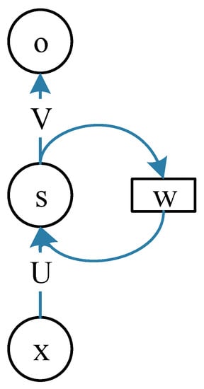
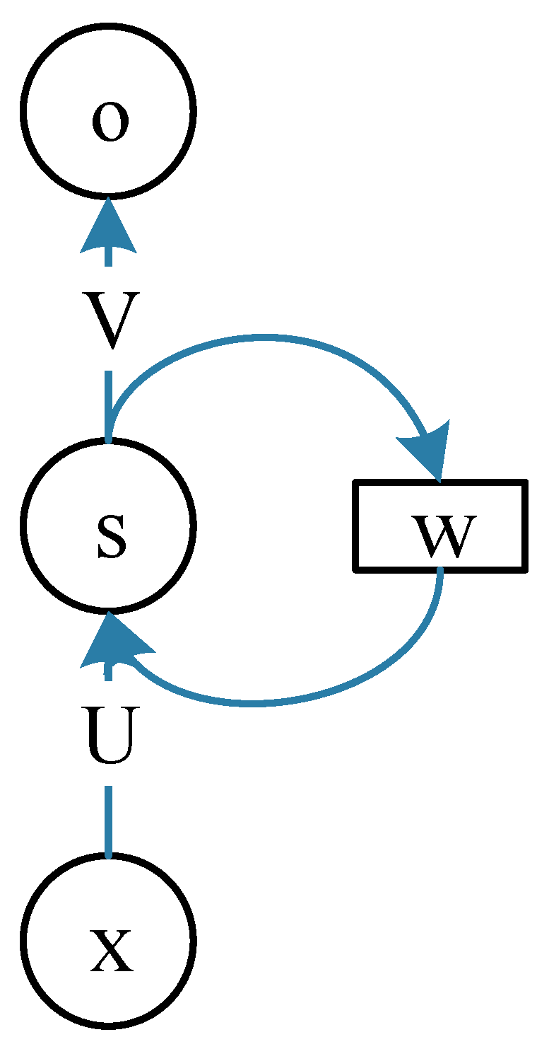
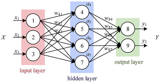
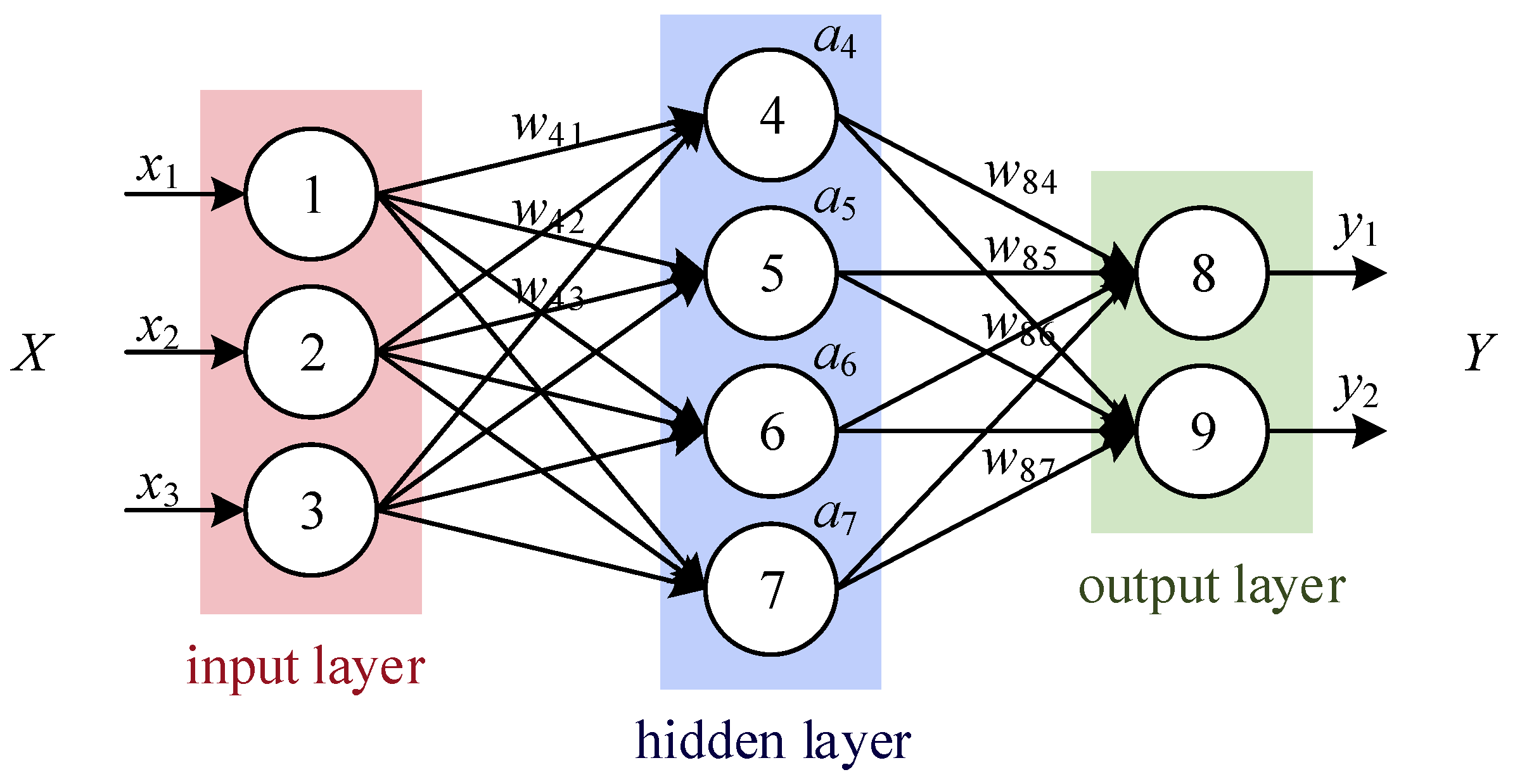
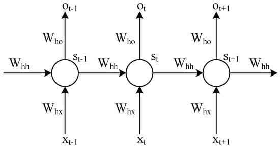
The prototype of Recurrent Neural Network was first introduced by John Hopfield, Michael I. Jordan defined the concept of Recurrent, and then Jeffery L, Elman proposed the earliest and the simplest Recurrent Neural Network with a single self-connected node at present. Recurrent Neural Network usually owns an input layer, a hidden layer and an output layer, as shown in Figure 1, and unlike traditional neural networks that only perform unidirectional propagation, Recurrent Neural Network has a memory function, and there is a loopback between the hidden layer units based on a time series which is expressed as the current output is influenced by the output of the previous moment. Recurrent Neural Network can be very effective in processing data with sequence characteristics, and can mine the effective information in the data. so Recurrent Neural Networks are now widely used in processing text, speech and other tasks. Figure 1 can be converted into Figure 2 when ignoring $W$, which shows that the structure is a fully connected neural network structure, through this figure, we can see that $X$ is a three-dimensional vector, $U$ denotes a three-row and four-column parameter matrix from the input layer to the hidden layer, $S$ denotes a four-dimensional vector of the hidden layer, $V$ represents a four-row and two-column parameter matrix from the hidden layer to the output layer, and $O$ represents a two-dimensional vector of the output layer. In Figure 1, $U$ represents the value from the input layer to the hidden layer, $S$ denotes the hidden layer output value, $W$ denotes the weight from the previous moment output to the current moment input, $V$ denotes the weight vector from the hidden layer to the output layer, and O represents the output vector of the output layer.

Figure 1. Recurrent Neural Network structure diagram.

Figure 2. Fully connected neural network structure.

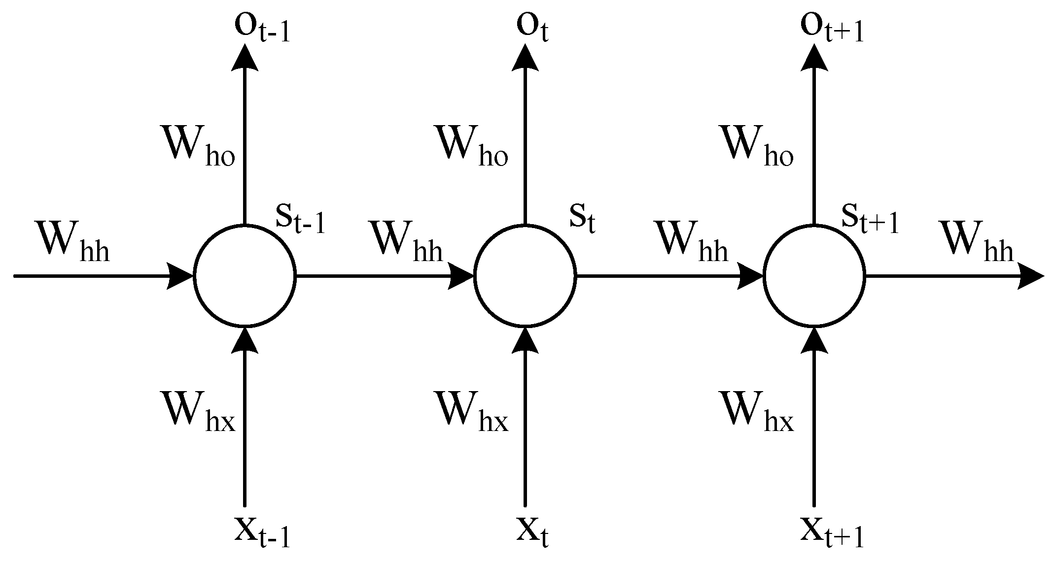
Expanding Recurrent Neural Network structure by the time line yields a graph of the hidden layer unit structure, and the connection structure between the hidden layer units of Recurrent Neural Network is illustrated in Figure 3. At moment $t$, the input of the hidden layer unit is $s_{t-1}$ and $x_t$, the value of the hidden layer unit is $s_t$, and the output is $o_t$.

Figure 3. Recurrent Neural Network hidden layer unit structure diagram.

From Figure 2, the forward calculation process of Recurrent Neural Network can be introduced as Equations (1) and (2)

$$s_t=f\left(W_{hh}\cdot x_t+W_{hh}\cdot s_{t-1}+b_s\right)$$

(1)

$$o_t=\sigma \left(W_{ho}\cdot s_t+b_o\right)$$

(2)

where $\sigma$ is the $sigmoid$ function, which is a common activation function in neural networks. $b$ is bias, $f$ is full connection layer.

3.2. Long Short-Term Memory Network

Because Recurrent Neural Network frequently fail owing to gradient explosion and disappearance, a new class of Recurrent Neural Networks called Long short-term memory network (LSTM) was developed to overcome this problem. Sepp Hochreiter and Jürgen Schmidhuber first proposed LSTM in 1997. LSTM has more input gates compared to recurrent neural networks, forgetting gate and output gate, which can get the corresponding weights and have different values at different moments with fixed parameters. Thus, LSTM can control the memory of the whole process better compared to recurrent neural networks, and thus successfully avoid the problems of gradient explosion and vanishing.

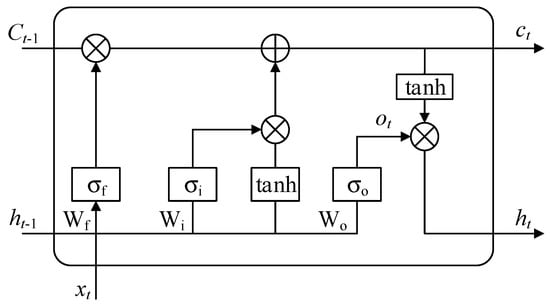
The cell state lies at the heart of the LSTM, with the horizontal line at the top of the graph running through the upper part of the graph. The cell states extend along with a straight line like a chain, and the linear interactions are small. Information can flow very easily. The LSTM can change information to the cell state according to the gate structure in Figure 4. It can be found that at time t, the LSTM cell owns three inputs, which are the input sequence $x_t$, the output of the previous step $h_{t-1}$ and the LSTM cell state $c_{t-1}$; there are two outputs, $h_t$, $c_t$; and three internal gates, which are the forgetting gate $f$, the input gate $i$ and the output gate $O$. The LSTM implements protection and control of cell states through three gate cells.

Figure 4. LSTM model structure diagram.

The work of LSTM can be divided into four steps.

(1) By selecting that unnecessary information should be eliminated from the cell state, the forgetting gate produces the outputs shown in Equation (3).

$$f_t=\sigma \left(W_f\cdot \left[h_{t-1},x_t\right]+b_f\right)$$

(3)

where $\sigma$ is the $sigmoid$ function, which is a common activation function in neural networks.

The output is f_t which is then multiplied point by point with the cell state of $c_{t-1}$. The data is between 0–1. If when the data is 0, it means that all information is discarded, and conversely when the data is 1, it means that all information is retained.

• $c_{t-1}$: Output of the previous moment of the cell state
• $h_{t-1}$: Template output from the previous moment
• $f_t$: Output of the Oblivion Gate
• $W_f:$ Weight matrix
• $b_f:$ Offset
• $\left[h_{t-1},x_t\right]$: two matrices stitched together

(2) The input gate has two parts that store information in the cell state: the first is the input gate layer’s decision on which there is information to update, and the second is a vector of optional values created by the layer to decide which information to add to those in the cell state. As in Equations (4) to (5)

$$i_t=\sigma \left(W_i\cdot \left[h_{t-1},x_t\right]+b_i\right)$$

(4)

$${\tilde{c}}_t=\tan h\left(W_c\cdot \left[h_{t-1},x_t\right]+b_c\right)$$

(5)

(3) Multiply the old state $c_{t-1}$ by the point $f_t$, indicating that the information that has been decided to be forgotten is discarded, and then add $i_t\ast {\tilde{c}}_t$, thus forming the new cell state $c_t$, which is the new optional value, scaled in size according to the state value. Equation (6).

$$c_t=f_t\ast c_{t-1}+i_t\ast {\tilde{c}}_t$$

(6)

(4) The output gate performs the output, and the cell state determines the output. As in Equations (7) to (8)

$$o_t=\sigma \left(W_o\cdot \left[h_{t-1},x_t\right]+b_o\right)$$

(7)

$$h_t=o_t\ast \tan h\left(c_t\right)$$

(8)

3.3. Back Propagation Neural Networks

Rumelhart [19] proposed the Back Propagation neural network, which solves the learning problem of multilayer neural networks. It is composed of three layers, including an input layer, a hidden layer, and an output layer, which has a wide range of applications. Firstly, the signal is transmitted from the input layer to the hidden layer through forward propagation and calculated in the hidden layer. Then the results of the hidden layer calculation are transmitted to the output layer and output. Finally, the results are compared with the expected values, and the error is corrected by back propagation. For example, Bai et al. [20], Fuh, K. H. et al., [21] employed the prediction model to medical, creep feed grinding, respectively. To facilitate the distinction, Back Propagation neural network model based on time series prediction is called Time Series-Back Propagation neural network; the Back Propagation neural network model based on impact factor prediction is called Impact Factor-Back Propagation neural network.

3.4. Grey Model (1,1)

Deng [22] fist introduced the Grey Model (1,1), which generated an approximation exponential rule by summarizing the original data and the modelling it. The model has been widely used in various area. For example, Liu et al. [23] and Wang et al. [24] employed the prediction model to tourism and construction. To facilitate the distinction, the Grey Model (1,1) is divided into Time Series-Grey Model (1,1) and Impact Factor-Grey Model (1,1). The modeling steps of Grey Model (1,1) are:

(1)

Build the original sequence, $X^0$ can be set to the original sequence:

$$X^{\left(0\right)}=\left[X^{\left(0\right)}\left(1\right),X^{\left(0\right)}\left(2\right),X^{\left(0\right)}\left(3\right),\cdots ,X^{\left(0\right)}\left(n\right)\right]$$

(9)

(2)

Calculate a cumulative sequence, generate a new sequence, set to $X^1$

$$X^{\left(1\right)}=\left[X^{\left(1\right)}\left(1\right),X^{\left(1\right)}\left(2\right),X^{\left(1\right)}\left(3\right),\cdots ,X^{\left(1\right)}\left(n\right)\right]$$

(10)

$$X^1\left(k\right)={{\displaystyle \sum }}_{j=1}^k{X}^0\left(j\right),j=1,2,3,\cdots ,k$$

(3)

Generate the mean and calculate its background value

$$Z^{\left(1\right)}\left(k\right)=\frac{1}{2}\left(X^{\left(1\right)}\left(k\right)+X^{\left(1\right)}\left(k-1\right)\right)$$

(11)

(4)

Construct matrices $B$ and $Y$.

$$B=\left[\begin{array}{c}-Z^{\left(1\right)}\left(1\right) 1\\ -Z^{\left(1\right)}\left(2\right) 1\\ ⋮\\ -Z^{\left(1\right)}\left(n\right) 1\end{array}\right],$$

(12)

$$Y=\left[\begin{array}{c}{X}^{\left(0\right)}\left(2\right)\\ X^{\left(0\right)}\left(3\right)\\ ⋮\\ X^{\left(0\right)}\left(n\right)\end{array}\right],$$

(13)

(5)

Construct differential equations

$$\frac{d{X}^{\left(1\right)}}{dt}+a{X}^{\left(1\right)}=u,$$

(14)

Solution of differential equation:

$$X^{\left(1\right)}\left(k+1\right)=\left[X^{\left(0\right)}\left(1\right)-\frac{u}{a}\right]e^{-ak}+\frac{u}{a},$$

(15)

Coefficient vector: $\widehat{a}={\left[a,u\right]}^T$.

3.5. Linear Regression

Francis Galton proposed the linear regression model, which uses regression equations to model the connection between one or more independent and dependent variables. The model has been widely used in various area. For example, Goldberger et al. [25] and Massie et al. [26] applied the predictive model to studies in biology, temperatures, construction and other industries, respectively. To facilitate the distinction, the Linear regression model based on time series prediction is called Time Series-Linear Regression; the Linear regression model based on impact factor prediction is called Impact Factor-Linear Regression. The modeling steps of Grey Model (1,1) are:

(1)

For a given sequence of n points,$\left(x_1,y_1\right)$, $\left(x_2,y_2\right)$…$\left(x_n,y_n\right)$ Let the linear regression equation be:

$$y=bx+a$$

(16)

(2)

The total distance from the point in the direction to the straight line can use ${{\displaystyle \sum _{i=1}^n\left[y_i-\left(a+b{x}_i\right)\right]}}^2$ to quantitatively describe, so it can be regarded as a binary function:

$$Q\left(a,b\right)={{\displaystyle \sum _{i=1}^n\left[y_i-\left(a+b{x}_i\right)\right]}}^2$$

(17)

(3)

Therefore, the problem of finding a straight line and making it closest to a point is transformed into finding two numbers $\widehat{a}$, $\widehat{b}$, so that the binary function $Q\left(a,b\right)$ reaches the minimum at $a=\widehat{a}$, $b=\widehat{b}$. Through formula derivation, finally we can obtain:

$$b=\frac{{\displaystyle \sum _{i=1}^n\left(x_i-\overline{x}\right)\left(y_i-\overline{y}\right)}}{{\displaystyle \sum _{i=1}^n\left(x_i-\overline{x}\right)}}$$

(18)

$$\overline{x}=\frac{1}{n}{\displaystyle \sum _{i=1}^n{x}_i}, \overline{y}=\frac{1}{n}{\displaystyle \sum _{i=1}^n{y}_i}, a=\overline{y}-b\overline{x}$$

4. Experimental Results and Analysis

4.1. Experimental Data Selection and Pre-Processing

Indicators for measuring logistics needs include logistics operations, cargo transportation, cargo turnover, logistics equipment, logistics employees, distribution operations and commodity inventory, etc. When selecting logistics indicators, we should not only consider the differences between indicators, but also consider the difficulty of obtaining each indicator. Therefore, we choose the freight volume as the measurement indicator. Since the volume of goods transported in reality is affected by more factors and the period of influencing factor values is long, this paper uses the annual unit for forecasting.

On the selection of impact factors, Huang et al. [5] selected 12 as observed variables including Gross Domestic Product, per capita disposable income, and investment in logistics fixed assets; Fan and Wu [27] chose Gross Domestic Product, the total social logistics cost, overall output value of one, two, three industries, freight volume, etc. to predict logistics needs. Du and Chen [28] employed Gross Domestic Product, postal services, and consumer consumption level as indicators for logistics needs forecasting; Han et al. [29] utilized Gross Domestic Product, overall social logistics cost, social fixed asset investment and import and export volume as indicators for logistics needs measurement and forecasting.

In view of the impact of the new crown pneumonia epidemic, many indicators are relatively lacking, so the impact factor is part of the indicator system constructed in the literature [5,27] as the attribute variables for the target prediction, in order to reflect the influence of the new crown pneumonia virus on logistics needs, and considering the integrity of the data, the more complete six indicators are selected as the impact factor. The influencing factors of logistics needs ($Y$) are Gross Domestic Product ($x_1$), urban disposable income per capita ($x_2$), overall retail sales of consumer products ($x_3$), overall import and export commerce ($x_4$), total postal and telecoms revenue ($x_5$) and cargo turnover ($x_6$).

The above data are presented in Table 1. First, the impact factors were normalized and calculated as follows:

$$X_u^{\prime }=\frac{X_u-X_{\min }}{X_{\max }-X_{\min }}$$

(19)

where $X_u$ denotes the original data; $X_u^{\prime }$ denotes the normalized data; $X_{\max }$ and $X_{\min }$ denote the maximum and minimum values of each variable, respectively. As shown in Table 2, the pre-processed data can be obtained by normalizing the data from the literature [1].

Table 1. Data on logistics requirements.

Year	Logistics Needs/Million Tons	Gross Domestic Product/Billion	Urban Disposable Income Per Capita/$	Overall Retail Sales of Consumer Products/Billion	Overall Import and Export Commerce/$ Billion	Total Postal and Telecoms Revenue/Billion	Cargo Turnover/Billion Tonne Kilometers
1998	5834	542	6650	226	12.08	20	100
1999	6456	588	7297	193	12.76	26.71	101
2000	5910	656	7985	234	16.44	37	140
2001	7550	728	8704	344	16.51	49	139
2002	8766	812	9021	401	16.64	36	79
2003	10,632	929	9933	451	20	41	91
2004	11,066	1133	11,021	525	24	43	101
2005	10,991	1519	12,434	743	26	47	100
2006	12,478	1798	13,924	865	29	55	109
2007	16,184	2190	16,153	1037	40	58	129
2008	17,158	3000	18,282	1273	51	68	132
2009	21,074	3744	20,238	1524	41	78	176
2010	22,947	4547	22,814	1864	60	90	219
2011	25,651	5619	26,451	2201	74	104	257
2012	26,145	6399	30,288	2521	86	114	301
2013	28,048	7153	33,662	2801	98	135	334
2014	30,449	7824	36,826	3162	125	194	359
2015	33,932	8510	39,961	3690	129	250	386
2016	36,767	9323	43,294	4117	109	378	387
2017	41,739	10,535	46,948	4547	138	557	448
2018	43,792	11,003	50,792	4765	193	647	487
2019	49,017	11,574	55,211	5247	289	1006	567
2020	49,346	12,142	57,971	4483	340	1271	570
2021	50,361	13,270	62,145	5111	430	1665	590

Table 2. Normalized data on logistics requirements.

Year	Logistics Needs/Million Tons	Gross Domestic Product/Billion	Urban Disposable Income Per Capita/$	Overall Retail Sales of Consumer Products/Billion	Overall Import and Export Commerce/$ Billion	Total Postal and Telecoms Revenue/Billion	Cargo Turnover/Billaion Tonne Kilometers
1998	5834	0.000	0.000	0.007	0.000	0.000	0.041
1999	6456	0.003	0.012	0.000	0.002	0.004	0.043
2000	5910	0.009	0.024	0.008	0.010	0.010	0.119
2001	7550	0.015	0.037	0.030	0.011	0.018	0.117
2002	8766	0.021	0.043	0.041	0.011	0.010	0.000
2003	10,632	0.030	0.059	0.051	0.019	0.013	0.023
2004	11,066	0.046	0.079	0.066	0.029	0.014	0.043
2005	10,991	0.077	0.104	0.109	0.033	0.016	0.041
2006	12,478	0.099	0.131	0.133	0.040	0.021	0.172
2007	16,184	0.129	0.171	0.167	0.067	0.023	0.098
2008	17,158	0.193	0.210	0.214	0.093	0.030	0.104
2009	21,074	0.252	0.245	0.263	0.069	0.035	0.190
2010	22,947	0.315	0.291	0.331	0.115	0.043	0.274
2011	25,651	0.399	0.357	0.397	0.148	0.051	0.348
2012	26,145	0.460	0.426	0.461	0.177	0.057	0.434
2013	28,048	0.519	0.487	0.516	0.206	0.070	0.499
2014	30,449	0.572	0.543	0.587	0.270	0.106	0.548
2015	33,932	0.626	0.600	0.692	0.280	0.140	0.601
2016	36,767	0.690	0.660	0.776	0.232	0.218	0.603
2017	41,739	0.785	0.726	0.861	0.301	0.326	0.722
2018	43,792	0.822	0.795	0.905	0.433	0.381	0.798
2019	49,017	0.867	0.875	1.000	0.663	0.599	0.955
2020	49,346	0.911	0.925	0.849	0.785	0.760	0.961
2021	50,361	1.000	1.000	0.973	1.000	1.000	1.000

4.2. Models Accuracy Evaluation

To validate the accuracy and reliability of the four models, Mean Absolute Percentage Error (MAPE), Root Mean Square Error (RMSE) and Mean Absolute Error (MAE) [30] were employed to assess the accuracy. Three error expressions are shown in (20) to (22), respectively.

$$MAE=\frac{1}{m}{\displaystyle \sum _{i=1}^m\left|\left(y_i-{\widehat{y}}_i\right)\right|}$$

(20)

$$RMSE=\sqrt{\frac{1}{m}{\displaystyle \sum _{i=1}^m{\left(y_i-{\widehat{y}}_i\right)}^2}}$$

(21)

$$MAPE=\frac{1}{m}{\displaystyle \sum _{i=1}^m\frac{\left|\left(y_i-{\widehat{y}}_i\right)\right|\cdot 100\%}{{\widehat{y}}_i}}$$

(22)

where $m$ denotes the number of predicted outcomes; ${\widehat{y}}_i$ denotes the actual value; $y_i$ denotes the predicted value.

4.3. Data Predictions and Results

To demonstrate the accuracy of Long short-term memory (LSTM) model prediction, we compare the LSTM with Grey Model, Back Propagation neural network model and linear regression model. Annual freight volume was used to create Grey Model, which was based on time series and impact variables, as well as the Back Propagation neural network model and linear regression model, all were trained and tested by MATLAB R2021b.

4.3.1. Prediction of LSTM Models

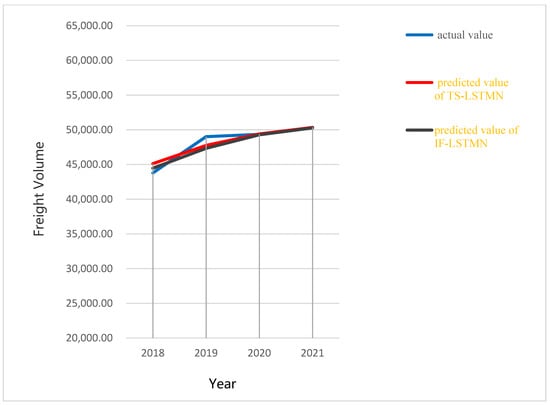
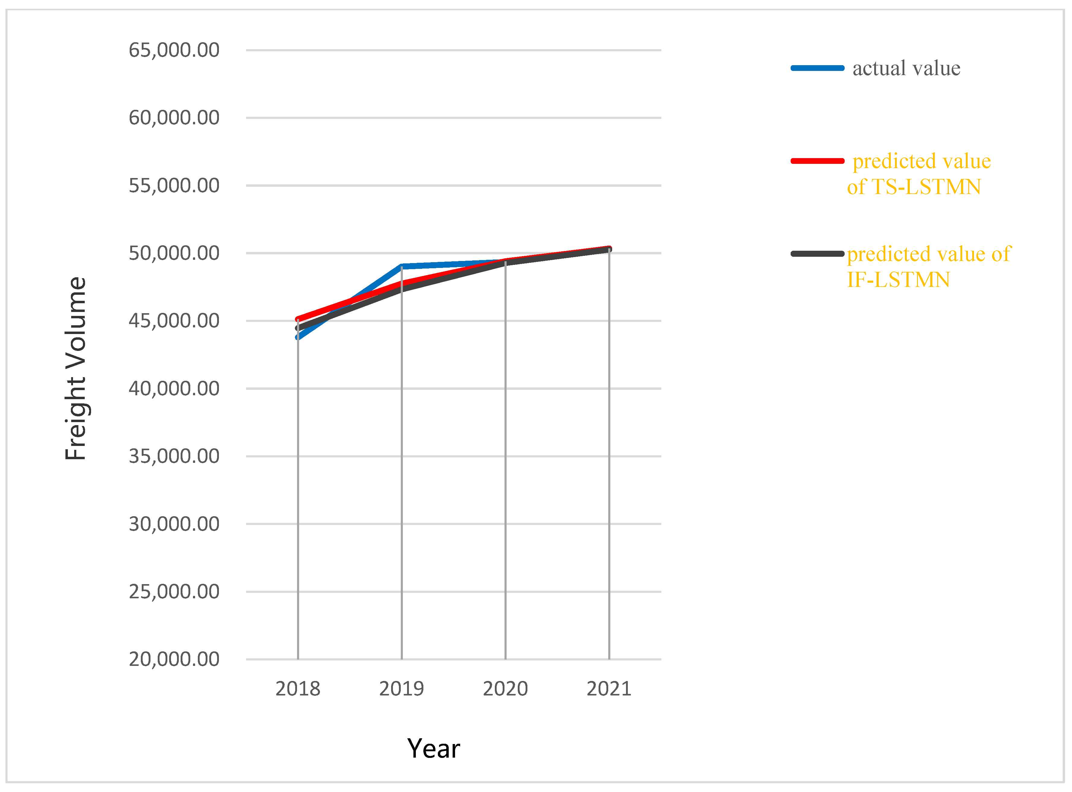
The setting of the hidden layer of Time Series-Long short-term memory network was determined by the grid search method [31] by selecting 19 hidden layer cells with 185 iterations, a step size of 1. 80% of the data set is used as a training set and the remaining 20% as a test set, and the optimization algorithm uses Adaptive Moment Estimation. As shown in Figure 5, the actual and predicted values are compared. The Time Series-Long short-term memory network model prediction error values are illustrated in Table 3.

Figure 5. LSTM model prediction graph.

Table 3. LSTM model prediction results.

Year	Real Value	Time Series-Long Short-Term Memory Network		Impact Factor-Long Short-Term Memory Network
		Predicted Value	Relative Error	Predicted Value	Relative Error
2018	43,792	45,130.3	0.0306	44,469.6	0.0155
2019	49,017	47,751	−0.0258	47,334	−0.0343
2020	49,346	49,404	0.0012	49,276.8	−0.0014
2021	50,361	50,341	−0.0004	50,276.2	−0.0017
MAPE/%		1.4490%		1.3200%
MAE		670.5762		628.6807
RMSE		921.6036		908.8091

The prediction model dimension of Impact Factor-Long short-term memory network model is then six dimensions input one dimension output, the Impact Factor-Long short-term memory network hidden layer unit is set to 23, the number of iterations is 250, the step size is 1, and the initial learning rate is 0.005. The prediction results are illustrated in Table 3.

After 2019, both time series and impact factor prediction of freight volume are gradually close to actual freight volume. This shows that LSTM has excellent prediction performance.

4.3.2. Prediction of Back Propagation Neural Network Models

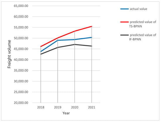
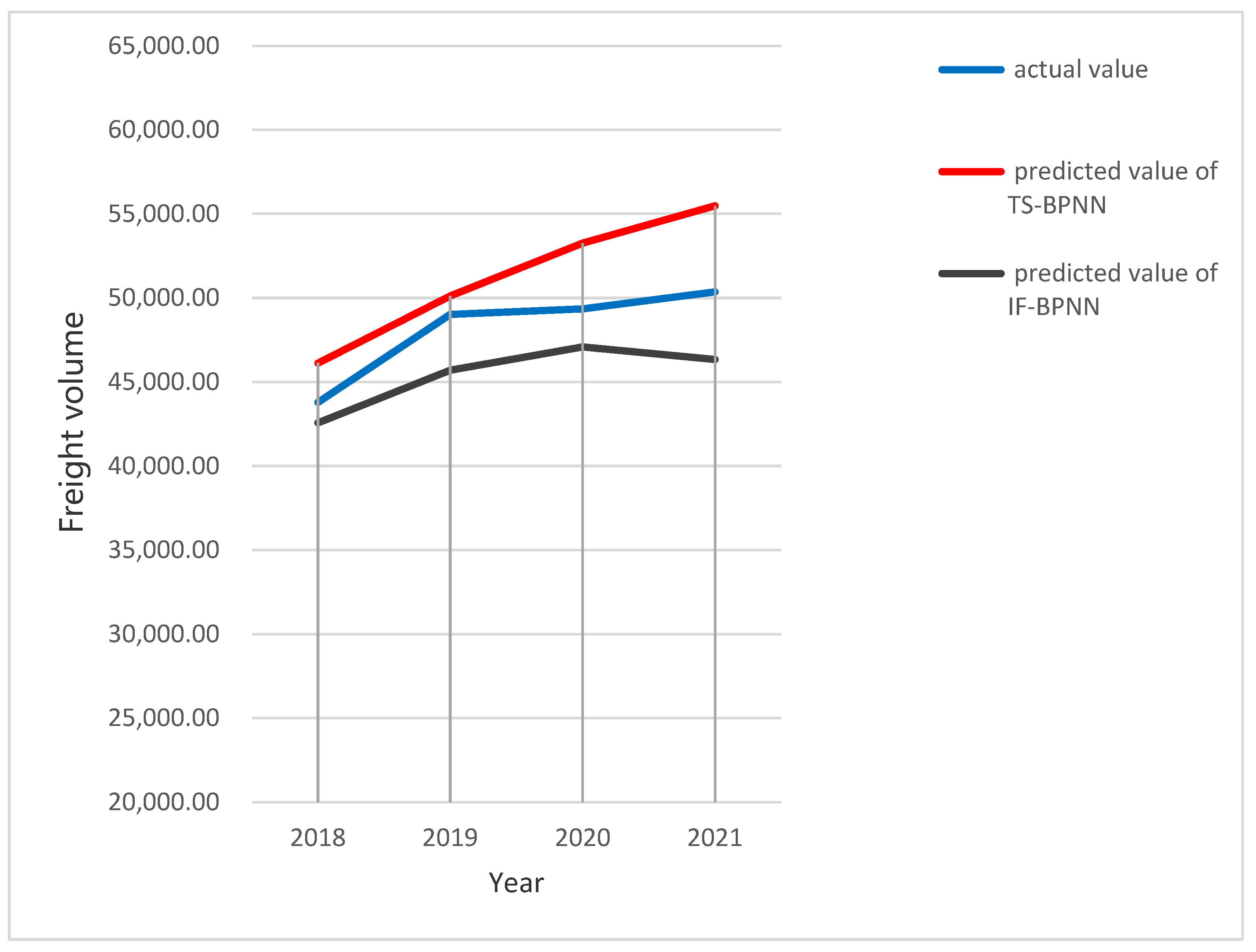
The Time Series-Back Propagation neural network model, based on empirical Equation (23) [32] and repeated training tests, uses a 3-layer network structure with 1 neuron in the input layer and 4 neurons in the hidden layer. The actual and predicted values are compared as shown in Figure 6, and the prediction error values of the Back Propagation neural network time series model are illustrated in Table 4.

Figure 6. Back Propagation neural network model predicted values.

Table 4. Back Propagation neural network model prediction results.

Year	Real Value	Time Series-Back Propagation Neural Network		Impact Factor-Back Propagation Neural Network
		Predicted Value	Relative Error	Predicted Value	Relative Error
2018	43,792	46,123	0.0532	42,568	−0.0073
2019	49,017	50,120.2	0.0225	45,704.6	−0.0373
2020	49,346	53,254.8	0.0792	47,089.4	−0.0266
2021	50,361	55,484.2	0.1017	46,339.1	−0.0159
MAPE/%		6.4169%		5.4982%
MAE		3116.5484		2688.7188
RMSE		3470.4602		2883.5193

Impact Factor-Back Propagation neural network, through the empirical formula and repeated training tests, owns the optimal prediction accuracy when the number of hidden layer neurons is determined as 12. Figure 6 shows Back Propagation neural network prediction model that is created.

It is discovered that there is a tiny discrepancy between the projected and real values of logistics needs size by plotting the actual and forecasted values. Both Time Series-Back Propagation neural network and Impact Factor-Back Propagation neural network are less accurate than LSTMN.

$$h=\sqrt{m+n}+a$$

(23)

where $h$ denotes the amount of hidden layer nodes, $m$ represents the amount of input layer nodes, $n$ represents the amount of output layer nodes, and $a$ denotes a regulation constant between 1 and 10.

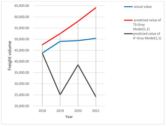
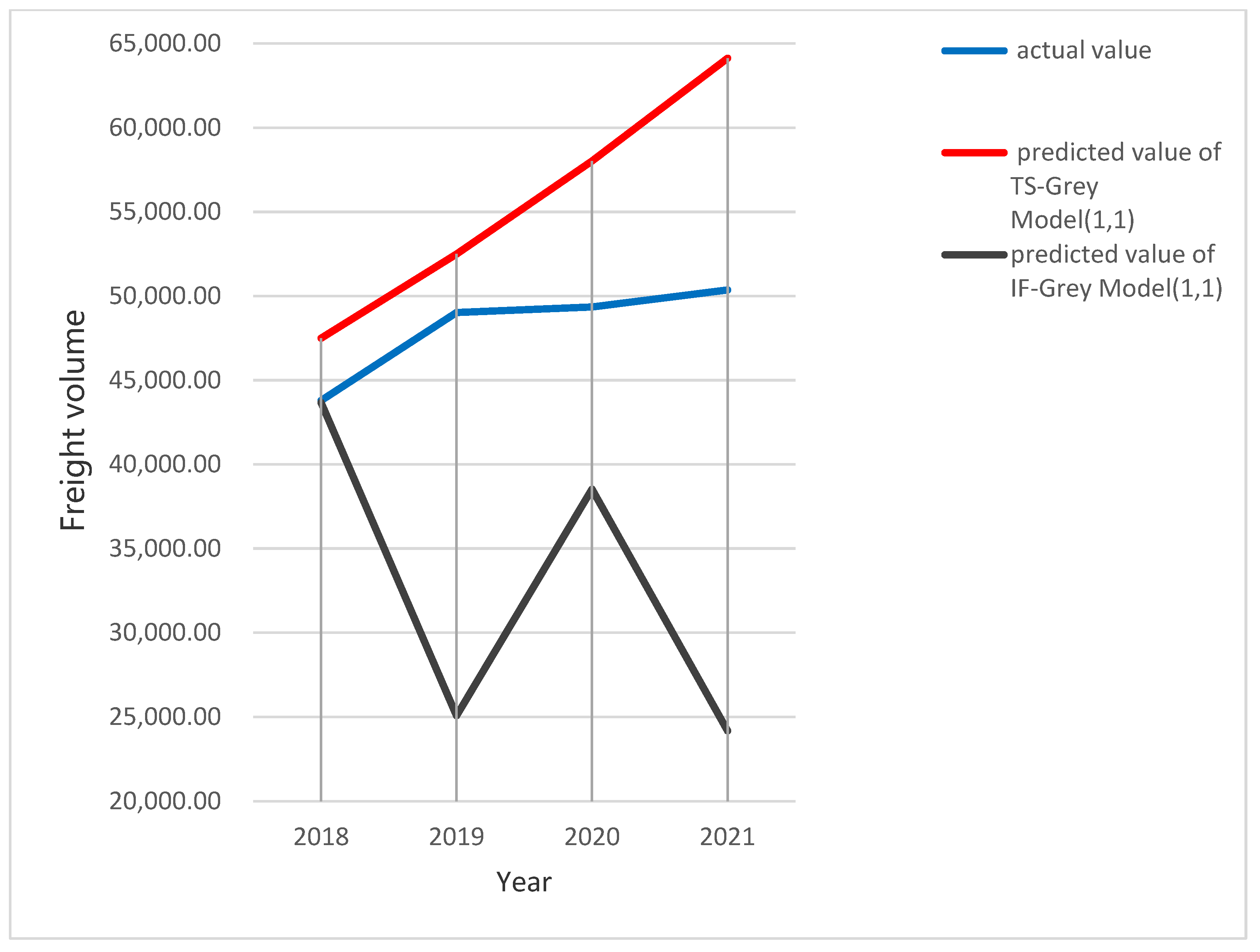
Figure 7 demonstrates a comparison of the actual and results of Grey Model (1,1), and Table 5 reveals the prediction fault values of Grey Model (1,1). Figure 7 can be observed that the anticipated values differ significantly from the actual ones. When compared with the neural network method, the accuracy of the traditional prediction method is lower than that of the neural network.

Figure 7. Grey model predicted values.

Table 5. Grey model prediction results.

Year	Real Value	Time Series-Grey Model (1,1)		Impact Factor-Grey Model (1,1)
		Predicted Value	Relative Error	Predicted Value	Relative Error
2018	43,792	47,496.5	0.0846	43,672.5	−0.0027
2019	49,017	52,496.7	0.0709	25,073	−0.4885
2020	49,346	58,023.4	0.1758	38,530	−0.2192
2021	50,361	64,131.83	0.2734	24,172	−0.5200
MAPE/%		15.1175%		30.7600%
MAE		7408.1075		15,267
RMSE		8565.9114		18,548

4.3.3. Linear Regression Model

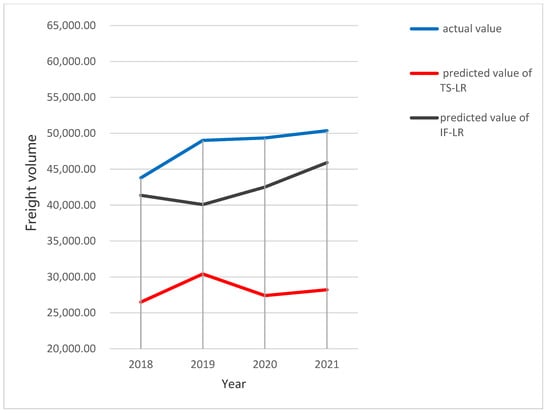
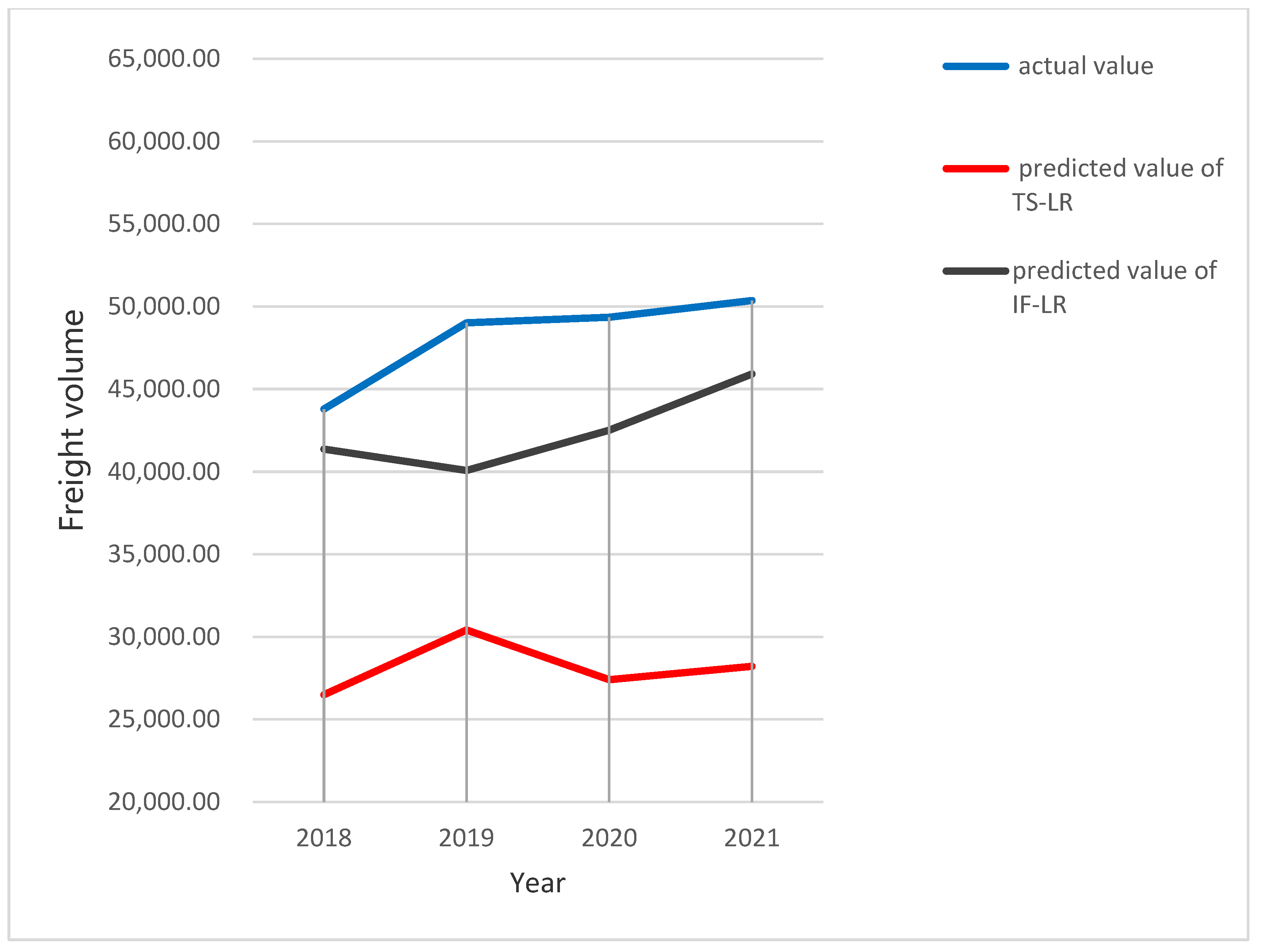
Figure 8 provides a comparison of the linear regression model’s actual and anticipated values, while Table 6 illustrates the model prediction error. Figure 8 demonstrates that the time series of logistics needs is not a linear function and there is also a large error in the multiple linear regression based on the impact factor predictions.

Figure 8. Linear regression model predicted values.

Table 6. Linear regression model prediction results.

Year	Real Value	Time Series-Linear Regression		Impact Factor-Linear Regression
		Predicted Value	Relative Error	Predicted Value	Relative Error
2018	43,792	26,501.8	−0.3948	41,363	−0.0555
2019	49,017	30,416.1	−0.3795	40,076	−0.1824
2020	49,346	27,409.6	−0.4518	42,514	−0.1385
2021	50,361	28,214.5	−0.4398	45,919	−0.0882
MAPE/%		41.4650%		11.6150%
MAE		19993.5		5661
RMSE		20,103.5911		6169.4633

As can be seen from Table 7 and Table 8, the MAE, RMSE and MAPE of the LSTM are the smallest between the four forecasting methods. Among them, the MAPE of time series and impact factor of LSTM network is only 2.2874% and 1.3200%. However, the linear regression model has the worst results, which shows that the single linear regression model is not suitable for predicting regional logistics needs. Compared with neural network prediction, traditional prediction methods have poor accuracy, which demonstrates that the LSTM has the best application and extension values among four models.

Table 7. Evaluation indicators for time series prediction results.

Models	RMSE	MAE	MAPE/%
LSTM	921.6036	670.5762	1.4490%
Grey Model (1,1)	8565.9114	7408.1075	15.1175%
Back Propagation neural network	3470.4602	3116.5484	6.4169%
Linear regression model	20,103.5911	19,993.5000	41.4650%

Table 8. Evaluation indicators for impact factor prediction results.

Models	RMSE	MAE	MAPE/%
LSTM	908.8091	628.6807	1.3200%
Grey Model (1,N)	18,548.0000	15,267.0000	30.7600%
Back Propagation neural network	2883.5193	2688.7188	5.4982%
linear regression	6169.4633	5661.0000	11.6150%

4.4. Prediction of Logistics Needs Scale

As shown in Table 3, Time Series-Long short-term memory network is better than Impact Factor-Long short-term memory network from 2019 to 2021, so the logistics needs for Changsha City 2022–2024 is forecasted by the established LSTM time series forecasting model, with predicted results of 512.752, 516.784 and 519.694 million tons, respectively, as illustrated in Table 9. Changsha City’s logistics needs will increase from 58.54 million tonnes in 1998 to 519.694 million tonnes in 2024, and the increase is very large. Although the epidemic is constantly repeated, driven by e-commerce, community group buying and other factors, logistics needs in Changsha city will increase, so the government and logistics companies should seize this opportunity to promote the recovery and development of the local economy. At the same time, epidemic prevention and disinfection of goods still cannot be taken lightly.

Table 9. Logistics needs scale from 2022 to 2024.

Year	Freight Volume
2022	51,275.2
2023	51,678.4
2024	51,969.4

5. Conclusions

Regional logistics demand prediction is employed for enterprise taking appropriate adjustment strategies and measures according to the prediction results, effectively avoiding risks, and seeking the maximum benefits. In the context of the ups and downs of the epidemic, if there is no effective prediction model for regional logistics demand, enterprises may not be able to make effective personnel and material scheduling, financial investment and other issues. For example, in the annual shopping carnival, if businesses cannot effectively predict this year’s sales volume, it will cause a large number of products and funds to be overstocked or the number of products to be insufficient, which will damage the interests of businesses. Therefore, the aim of the research is to select an effective model in term of e-commerce and the post-epidemic era by analyzing and comparing Grey Model (1,1), Back Propagation neural network, Linear regression, and Long Short-Term Memory (LSTM) to predict the regional logistics needs of Changsha city. Meanwhile, the LSTM network has the best results among the four models. The results show that LSTM model has a smaller prediction error and more stable prediction results due to its effective use of time series.

However, there are still several drawbacks. The first is that the selection of the index system is somewhat subjective, and the regional logistics needs will also be affected by, for example, the level of logistics service. Therefore, in future research, it is worth to extend the regional logistics forecasting index system to other diversified angles. Secondly, the approaches chosen for comparison have certain drawbacks, and it is evident that forecasting methods such as mixed forecasting models and support vector machines are equally viable options. In the future, we should add different forecasting models. Then, the selected region also has certain limitations, and does not verify whether the logistics demand of all regions will increase under the influence of epidemic and e-commerce. Finally, it is that this paper has not been able to optimize the LSTM network so that it can achieve the idealized results. Thus, it is necessary to take more attention to the related work so as to further study.

References

- Geng, J.; Li, C. Empirical research on the spatial distribution and determinants of regional e-commerce in China: Evidence from Chinese provinces. Emerg. Mark. Finance Trade 2020, 56, 3117–3133. [Google Scholar] [CrossRef] [Scilit]
- Mohdhar, A.; Shaalan, K. The future of e-commerce systems: 2030 and beyond. In Recent Advances in Technology Acceptance Models and Theories; Springer: Cham, Switzerland, 2021; pp. 311–330. [Google Scholar]
- Mladenow, A.; Bauer, C.; Strauss, C. “Crowd logistics”: The contribution of social crowds in logistics activities. Int. J. Web Inf. Syst. 2016, 12, 379–396. [Google Scholar] [CrossRef] [Scilit]
- Yu, N.; Xu, W.; Yu, K.L. Research on regional logistics needs forecast based on improved support vector machine: A case study of Qingdao city under the New Free Trade Zone Strategy. IEEE Access 2020, 8, 9551–9564. [Google Scholar] [CrossRef] [Scilit]
- Huang, L.; Xie, G.; Zhao, W.; Gu, Y.; Huang, Y. Regional logistics needs forecasting: A BP neural network approach. Complex Intell. Syst. 2021, 1–16. [Google Scholar] [CrossRef] [Scilit]
- Samvedi, A.; Jain, V. A grey approach for forecasting in a supply chain during intermittentdisruptions. Eng. Appl. Artif. Intell. 2013, 26, 1044–1051. [Google Scholar] [CrossRef] [Scilit]
- Sheu, J.B.; Kundu, T. Forecasting time-varying logistics distribution flows in the One Belt-One Road strategic context. Transp. Res. Part E Logist. Transp. Rev. 2018, 117, 5–22. [Google Scholar] [CrossRef] [Scilit]
- Nuzzolo, A.; Comi, A. City logistics planning: Needs modelling requirements for direct effect forecasting. Procedia Soc. Behav. Sci. 2014, 125, 239–250. [Google Scholar] [CrossRef] [Scilit]
- Choi, T.M.; Wen, X.; Sun, X.; Chung, S.H. The mean-variance approach for global supply chain risk analysis with air logistics in the blockchain technology era. Transp. Res. Part E Logist. Transp. Rev. 2019, 127, 178–191. [Google Scholar] [CrossRef] [Scilit]
- He, Y.; Liu, N. Methodology of emergency medical logistics for public health emergencies. Transp. Res. Part E Logist. Transp. Rev. 2015, 79, 178–200. [Google Scholar] [CrossRef] [Scilit]
- Guo, H.; Guo, C.; Xu, B.; Xia, Y.; Sun, F. MLP neural network-based regional logistics needs prediction. Neural Comput. Appl. 2021, 33, 3939–3952. [Google Scholar] [CrossRef] [Scilit]
- Li, B.; Zhang, J.; He, Y.; Wang, Y. Short-term load-forecasting method based on wavelet decomposition with second-order gray neural network model combined with ADF test. IEEE Access 2017, 5, 16324–16331. [Google Scholar] [CrossRef] [Scilit]
- Jaipuria, S.; Mahapatra, S.S. An improved needs forecasting method to reduce bullwhip effect in supply chains. Expert Syst. Appl. 2014, 41, 2395–2408. [Google Scholar] [CrossRef] [Scilit]
- Prakash, C.; Barua, M.K. Integration of AHP-TOPSIS method for prioritizing the solutions of reverse logistics adoption to overcome its barriers under fuzzy environment. J. Manuf. Syst. 2015, 37, 599–615. [Google Scholar] [CrossRef] [Scilit]
- Wang, D.Z.; Lang, M.X.; Sun, Y. Evolutionary game analysis of co-opetition relationship between regional logistics nodes. J. Appl. Res. Technol. 2014, 12, 251–260. [Google Scholar] [CrossRef] [Scilit]
- Zendehboudi, A.; Baseer, M.A.; Saidur, R. Application of support vector machine models for forecasting solar and wind energy resources: A review. J. Clean. Prod. 2018, 199, 272–285. [Google Scholar] [CrossRef] [Scilit]
- Hu, B. Application of evaluation algorithm for port logistics park based on PCA-SVM model. Pol. Marit. Res. 2018, 3, 29–35. [Google Scholar] [CrossRef] [Scilit]
- Wang, Q.M.; Fan, A.W.; Shi, H.S. Network traffic prediction based on improved support vector machine. Int. J. Syst. Assur. Eng. Manag. 2017, 8, 1976–1980. [Google Scholar] [CrossRef] [Scilit]
- Rumelhart, D.E.; Hinton, G.E.; Williams, R.J. Learning representations by back-propagating errors. Nature 1986, 323, 533–536. [Google Scholar] [CrossRef] [Scilit]
- Bai, Y.; Jin, Z. Prediction of SARS epidemic by BP neural networks with online prediction strategy. Chaos Solitons Fractals 2005, 26, 559–569. [Google Scholar] [CrossRef] [Scilit]
- Fuh, K.H.; Wang, S.B. Force modeling and forecasting in creep feed grinding using improved BP neural network. Int. J. Mach. Tools Manuf. 1997, 37, 1167–1178. [Google Scholar] [CrossRef] [Scilit]
- Deng, J.L. Control problems of grey system. Syst. Control Lett. 1982, 1, 5. [Google Scholar]
- Liu, X.; Peng, H.; Bai, Y.; Zhu, Y.; Liao, L. Tourism flows prediction based on an improved grey GM (1, 1) model. Procedia Soc. Behav. Sci. 2014, 138, 767–775. [Google Scholar] [CrossRef] [Scilit]
- Wang, X.; Chen, Z.; Yang, C.; Chen, Y. Gray predicting theory and application of energy consumption of building heat-moisture system. Build. Environ. 1999, 34, 417–420. [Google Scholar] [CrossRef] [Scilit]
- Goldberger, A.S. Best linear unbiased prediction in the generalized linear regression model. J. Am. Stat. Assoc. 1962, 57, 369–375. [Google Scholar] [CrossRef]
- Massie, D.R.; Rose, M.A. Predicting daily maximum temperatures using linear regression and Eta geopotential thickness forecasts. Weather Forecast. 1997, 12, 799–807. [Google Scholar] [CrossRef] [Scilit]
- Fan, S.X.; Wu, B. Prediction analysis for logistics needs based on multiple kernels. Ind. Eng. Manag. 2018, 23, 40–44. [Google Scholar]
- Du, B.; Chen, A. Research on Logistics Needs Forecasting Based on the Combination of Grey GM (1, 1) and BP Neural Network. In Proceedings of the 5th Annual International Conference on Network and Information Systems for Computers (ICNISC2019), Wuhan, China, 19–20 April 2019; IOP Publishing: Bristol, UK, 2019; Volume 1288, p. 012055. [Google Scholar]
- Han, H.J.; Han, J.B.; Zhang, R. Study on logistics needs forecasting model based on fuzzy cognitive map. Syst. Eng. Theory Pract. 2019, 39, 1487–1495. [Google Scholar]
- Brailsford, T.J.; Faff, R.W. An evaluation of volatility forecasting techniques. J. Bank. Finance 1996, 20, 419–438. [Google Scholar] [CrossRef] [Scilit]
- Pedregosa, F.; Varoquaux, G.; Gramfort, A.; Michel, V.; Thirion, B.; Grisel, O.; Blondel, M.; Prettenhofer, P.; Weiss, R.; Dubourg, V.; et al. Scikit-learn: Machine learning in Python. J. Mach. Learn. Res. 2011, 12, 2825–2830. [Google Scholar]
- Chen, M. MATLAB Neural Network Principles and Examples of Fine Solution; Tsinghua University Press: Beijing, China, 2013; pp. 156–158. [Google Scholar]
Publisher’s Note: MDPI stays neutral with regard to jurisdictional claims in published maps and institutional affiliations. |
© 2022 by the authors. Licensee MDPI, Basel, Switzerland. This article is an open access article distributed under the terms and conditions of the Creative Commons Attribution (CC BY) license (https://creativecommons.org/licenses/by/4.0/).