Methodology for Interactive Labeling of Patched Asphalt Pavement Images Based on U-Net Convolutional Neural Network

Abstract

Image recognition based on deep learning generally demands a huge sample size for training, for which the image labeling becomes inevitably laborious and time-consuming. In the case of evaluating the pavement quality condition, many pavement distress patching images would need manual screening and labeling, meanwhile the subjectivity of the labeling personnel would greatly affect the accuracy of image labeling. In this study, in order for an accurate and efficient recognition of the pavement patching images, an interactive labeling method is proposed based on the U-Net convolutional neural network, using active learning combined with reverse and correction labeling. According to the calculation results in this paper, the sample size required by the interactive labeling is about half of the traditional labeling method for the same recognition precision. Meanwhile, the accuracy of interactive labeling method based on the mean intersection over union (mean_IOU) index is 6% higher than that of the traditional method using the same sample size and training epochs. In addition, the accuracy analysis of the noise and boundary of the prediction results shows that this method eliminates 92% of the noise in the predictions (the proportion of noise is reduced from 13.85% to 1.06%), and the image definition is improved by 14.1% in terms of the boundary gray area ratio. The interactive labeling is considered as a significantly valuable approach, as it reduces the sample size in each epoch of active learning, greatly alleviates the demand for manpower, and improves learning efficiency and accuracy.

1. Introduction

With the continuous advancement of highway engineering globally, an increasing road mileage has entered the maintenance stage. In-situ inspections are necessitated in decision-making on the maintenance strategies [1], which calls for efficient and accurate methods to evaluate the pavement technical condition. A rapid and accurate recognition of distress types and evaluation of severity play a critical role in the pavement maintenance engineering. The traditional road condition detection system, however, has mainly relied on manual operation, which is labor-intensive and can be strongly affected by personnel subjectivity, hence the lack of accuracy and efficiency. The automatic detection methods have become an indispensable component of pavement condition detection in order to improve this situation [2,3,4]. The image identification technique based on deep learning offers the benefit of high precision, among other approaches. Chen et al. [5] applied the graph cutting algorithm to segment the region and surface of the graph via an optimal path identified by minimizing the boundary and region energy function. Sezer et al. [6,7] applied the AlexNet model to the field of detecting solder paste defects. After optimizing the algorithm, the tests on six types of solder paste defects showed that the network provided a good performance on defect detection.

It is important to mention, despite considerable progresses made in the field of pavement crack detection, the deep learning method still requires a large amount of image-based labeling data for model training [8,9]. The labeling work is known to be time-consuming and laborious, and the imbalanced categorical data of the training set would result in a poorly trained model. Some researchers artificially select samples with high value and abundant information and add them to the labeled samples after labeling in order to improve the accuracy of network recognition [10]. This method is called active learning, which is generally comprised of two modules of learning and selection [11]. The learning module is applied for learning the characteristics of the sample data. In the selection module, samples are screened and labeled manually, and then added to the data sets in multiple batches to train the recognition ability of the learning module. The introduction of active learning method into deep learning allows to reduce the cost of manual labeling as much as possible [12]. Qin et al. significantly improved the performance of an active learning algorithm by comprehensively considering the information and representativeness of samples, formulating richness constraints, and effectively screening out valuable samples [13]. Nevertheless, it is important to realize that these methods are still largely subjective in selecting samples [14].

In order to reduce the dependence of deep learning network on the huge number of samples and alleviate the subjectivity of sample selection in active learning method, an interactive labeling method based on active learning is proposed for image recognition of pavement distress patching. Compared with the existing image recognition work, the interactive labeling method has the potential to improve the efficiency and accuracy. The present paper is organized as follows. In Section 2, the U-Net neural network for predicting patched asphalt pavement images is preliminarily constructed based on image preprocessing and network training. Section 3 describes the improvement of sample quality by reverse labeling and active correction, thus completing the interactive labeling. In Section 4, the prediction results are obtained by the interactive labeling method, the parameter analysis is provided, and the advantage of the method is visualized in case comparison.

2. Pavement Distress Identification System Based on U-Net Convolutional Neural Network

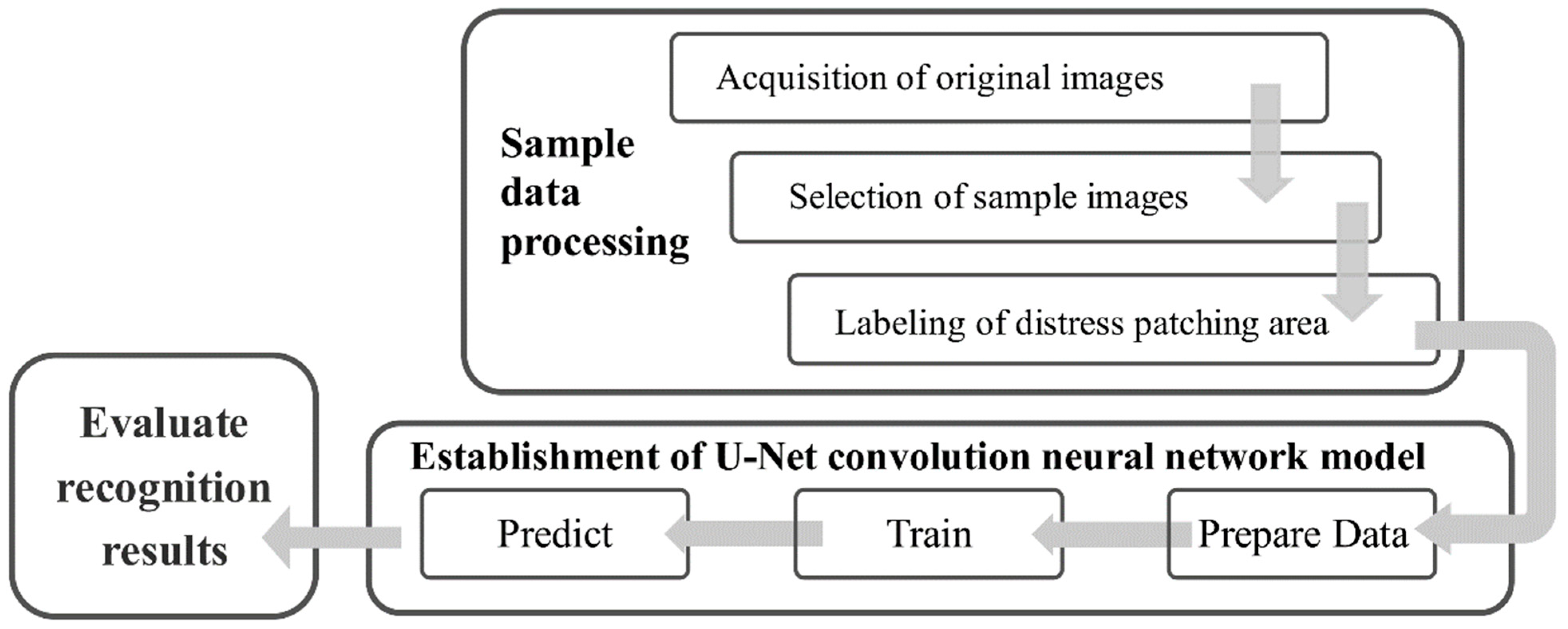
In this study, the pavement distress identification system is developed based on the U-Net convolution neural network that has been widely used in the medical field. Figure 1 outlines the three steps of the implementation:

(1) Sample data set processing, which aims to label the extracted image with the patch boundary information.

(2) Image segmentation based on U-Net deep learning network model, that is, the sample data set is divided into training and test sets by the ratio of 0.8 to 0.2, the former for network training and the latter for testing the ability of network segmentation.

(3) Evaluation of network identification ability, which aims at identifying randomly selected samples and evaluating the network identification ability based on the identification results, as well as the representativeness and richness of samples.

2.1. Image Preprocessing of Patched Asphalt Pavement

In this study, a line-scan digital camera equipped on a highway inspection vehicle was applied to acquire the original image of pavement surface by line scanning. The scanning width was 2 m and the obtained images had a resolution of 2048 by 2000 pixels. The training set was prepared by labeling the original images of pavement surface.

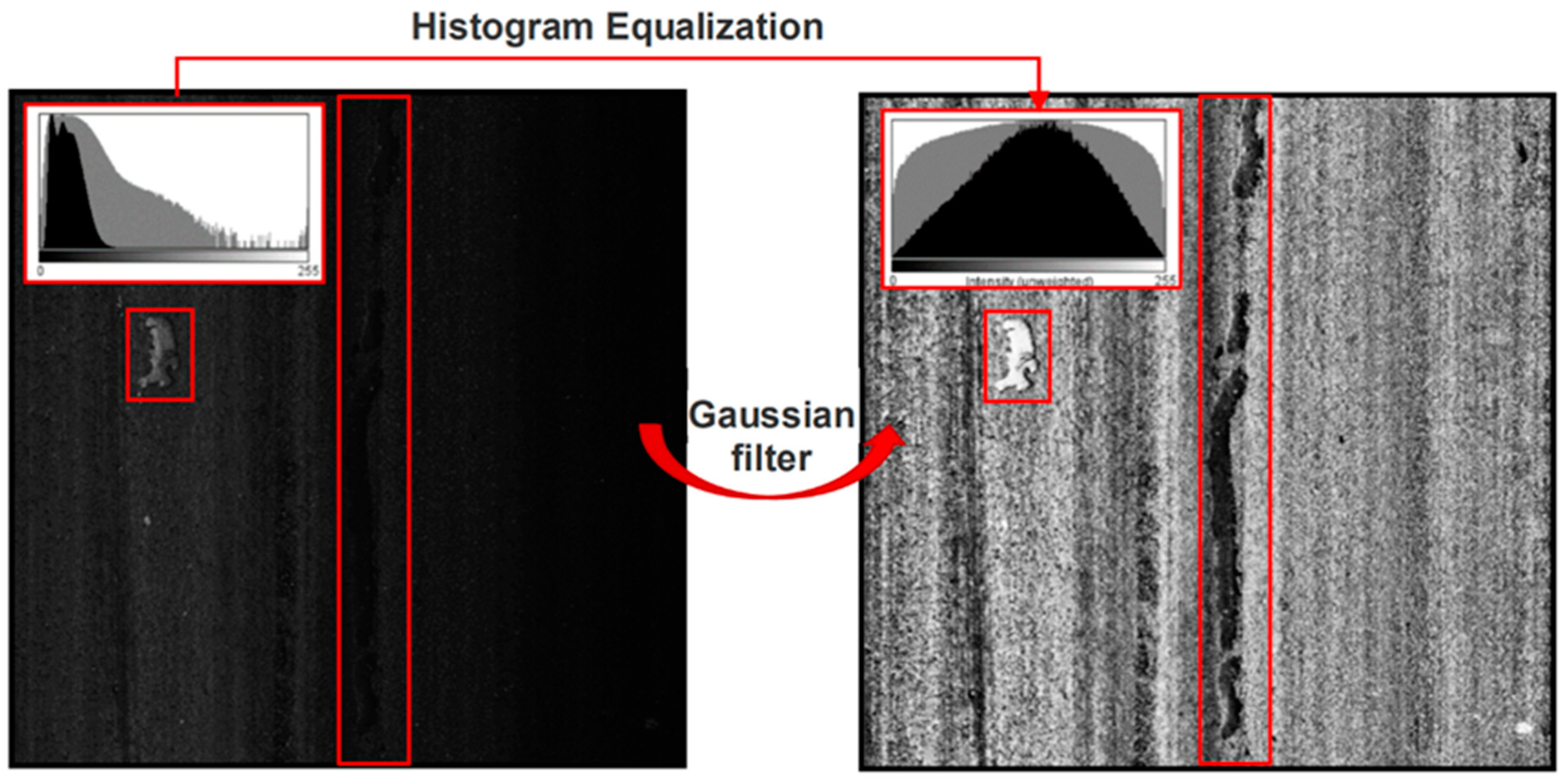
Although most of the distress images were sufficiently clear, some were difficult to identify the precise boundary of the patched area due to the influence of adverse environment during image collection (e.g., poor lighting conditions, changes in pavement surface reflection caused by water marks), and in certain cases it was challenging to confirm whether there was a distress patching. For these practical reasons, image preprocessing was of particular importance. In this paper, two Gaussian filters were used to equalize the original road image in a straight direction, namely, denoising and defogging [15,16]. This approach combined the image spatial information with the adjacent pixel information to smooth the image in filtering noise, and at the same time preserved the edge and enhanced the image details [17,18,19]. Application of the filters improved the recognition of the patch boundary and reduced the interference of background brightness to the marking process, as shown in Figure 2.

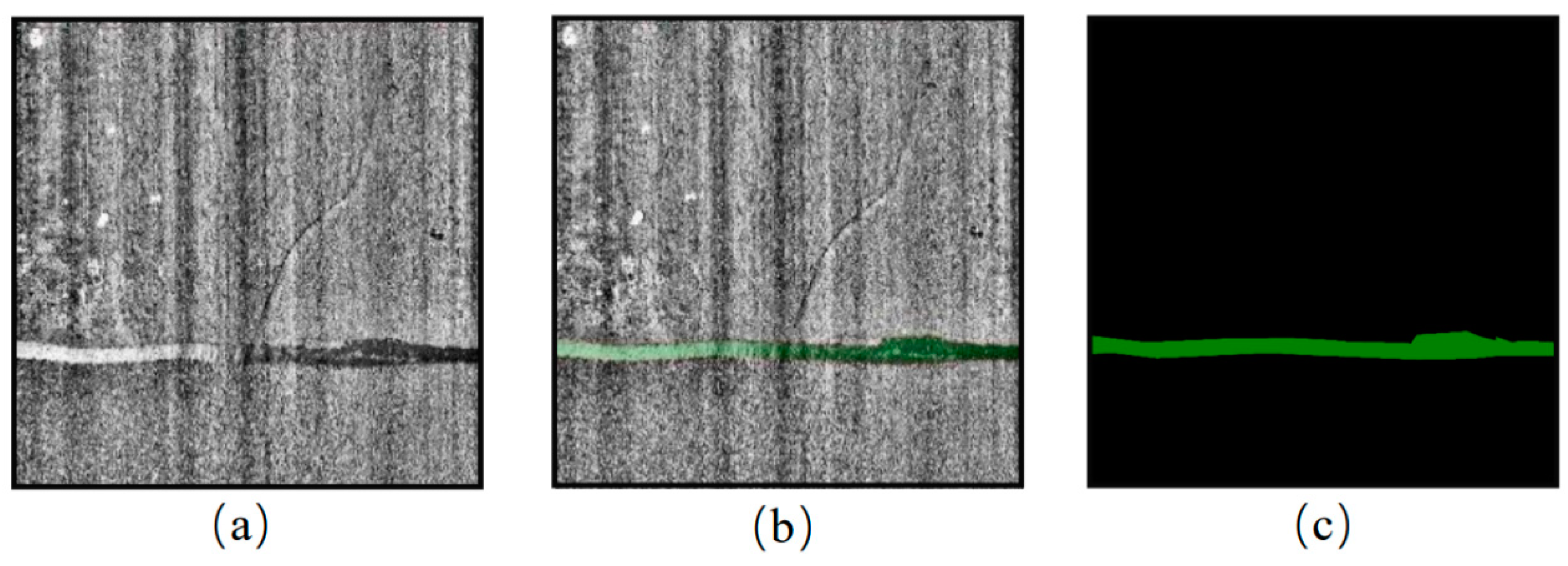
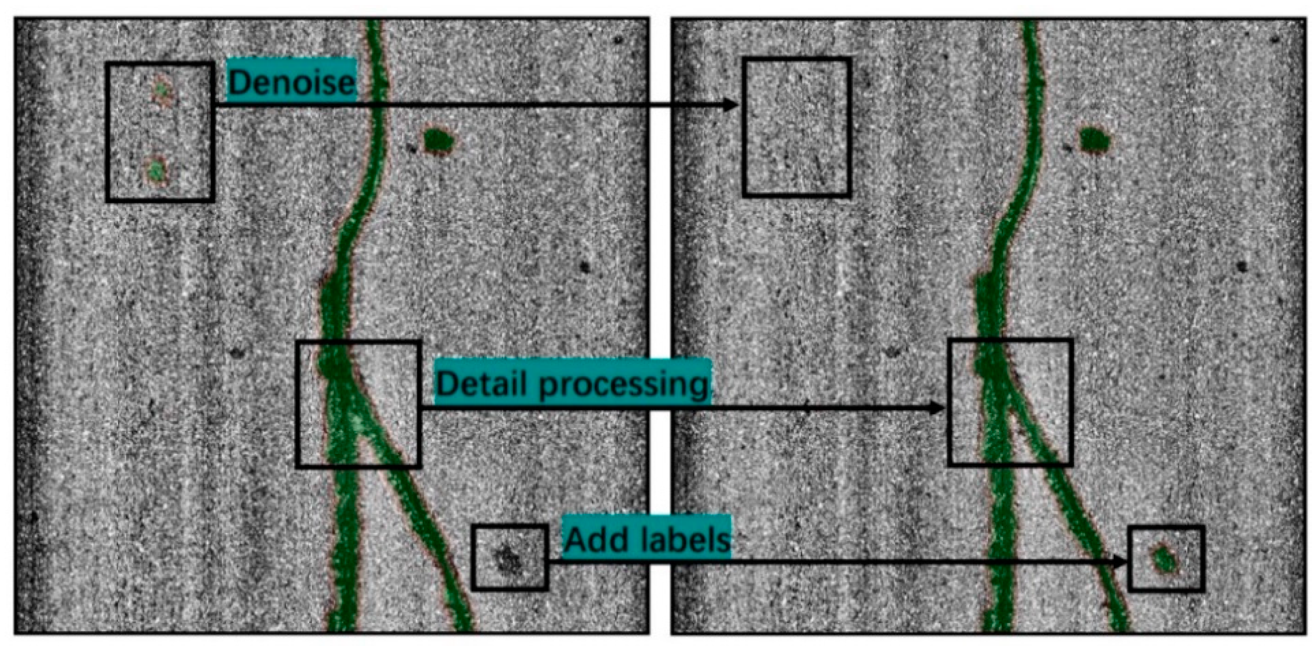
Next, the preprocessed images were labeled with the pavement distress area, as shown in Figure 3a. Traditional labeling methods, such as YOLO, Faster RCNN, and SSD [20,21]; usually the labeled images or outline of the approximate distress areas were completed in a direct manner, and the labeling accuracy could be relatively poor. Given this, the semantic segmentation labeling method [22] was adopted; that is, labeling was conducted by professionals with rich experience in pavement inspection and maintenance for the purpose of accurate pavement distress areas in terms of geometry (shape and scale) of the distress edges, as shown in Figure 3b. Finally, the labeled images were vectorized for training the convolutional neural network and prediction, Figure 3c.

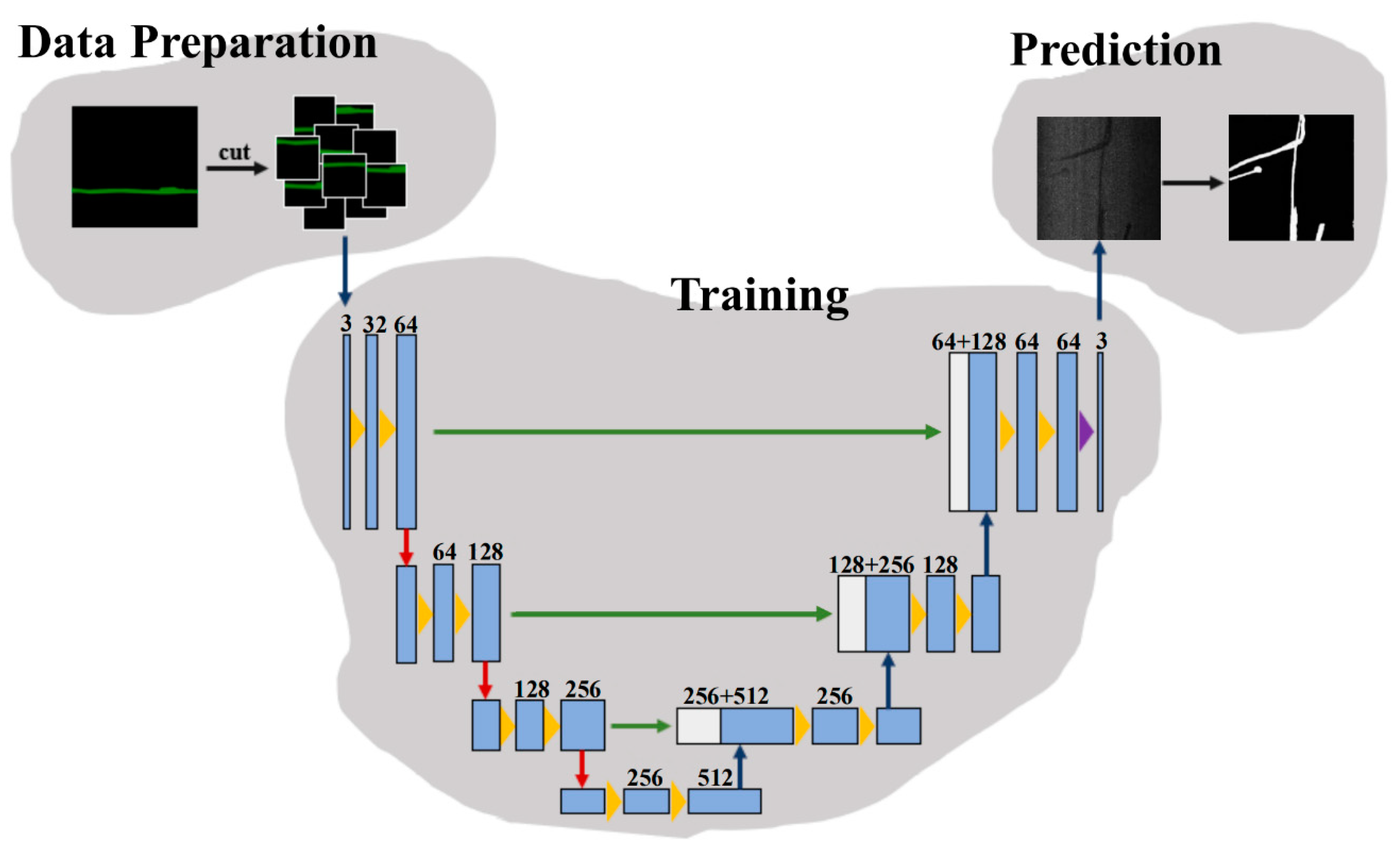
2.2. U-Net Convolution Neural Network Model

The U-Net convolutional neural network has been widely applied in medical image segmentation and recognition [23]. This network includes two main parts of convolutional coding and decoding units. Down-sampling is carried out in the convolutional coding unit, and the deconvolution operation is performed in the decoding unit to up-sample the feature image [24]. As shown Figure 4, U-Net down-samples four times and symmetrically up-samples four times, so as to restore the high-level semantic feature map to the resolution of the original image. The construction process of deep learning network based on the U-Net model is divided into three steps: (a) data preparation, in which the training sample set is prepared by random selection in the first epoch of recognition; (b) training, in which the network is trained through multiple epochs of learning; and (c) prediction, in which the network is to identify and segment the specified object.

In the process of “Data Preparation”, the original and labeled images are cropped into blocks of 512 by 512 pixels using a Python script. The step size of the cropping is set to 256 pixels to clean the invalid image data, which helps reduce the number of images involved in learning and improved learning efficiency. The training set is generated by randomly selecting 80% of the images, and the remaining 20% makes up the verification set that is used to automatically evaluate the learning progress of the network. The network training will then work through the images included in the training set for several epochs. Subsequent to each epoch, the algorithm will automatically compare the learning outcomes against the labeling results of the test set to calculate the mean_IOU index, which is positively related to the neural network accuracy and can be updated in real time. Generally, after several epochs of learning, the mean_IOU index can ascend to a high level, and the learning can be stopped when an increase in this index is marginal; additional learning may result in a negative increment in the index. Completion of the network training is followed by its verification via comparison between predicted and actual results.

3. Interactive Image Labeling

Generally speaking, the deep learning network needs a large sample size in training, which leads to tremendous labor and time requirements in image labeling. The active learning method provides a good option to alleviate such burden. Yet it focuses on selecting some information-rich data, which are insufficient to represent the characteristics of the whole data resulting in a poor generalization performance of the model. Moreover, the accuracy of recognition results is not directly proportional to the number of samples fed in [25]. In order to deal with this generally existing deficiency, using the images of asphalt pavement distress patches, this study proposes an interactive labeling method that features a two-part process of reverse labeling and correction labeling.

3.1. Reverse Labeling of Pavement Distress Images

Reverse labeling is a key step in the process of interactive labeling. It can be seen from the above discussion that the sample size directly affects the outcome of active learning. It is difficult to establish a connection between the manual selection and the neural network, as there is subjectivity involved in processing samples. Reverse labeling can help researchers find out the shortcomings and errors in neural network recognition, and improve the efficiency and accuracy of manual sample correction. It consisted of three steps. First, the gray image of the predicted result is segmented using a threshold value. Secondly, the image background after segmentation (in black) is removed, and the remaining (in white) is combined with the original image in the form of a mask. Finally, the boundary of the white portion of the image is traced and editing points are added for adjustment and modification. It is noted that the efficiency of reverse labeling can be potentially improved by integrating this process in a labeling software.

As previously mentioned, threshold segmentation is a commonly used image segmentation method, in which the difference in gray characteristics between the target object to be extracted and its background in the image is applied. The grayscale of the image is divided into two or more intervals by setting the appropriate gray threshold, in order to determine the meaningful region or the boundary of the segmented object [26]. Generally, the gray value continuously changing from black to white is discretized within the gray interval of 0 to 255.

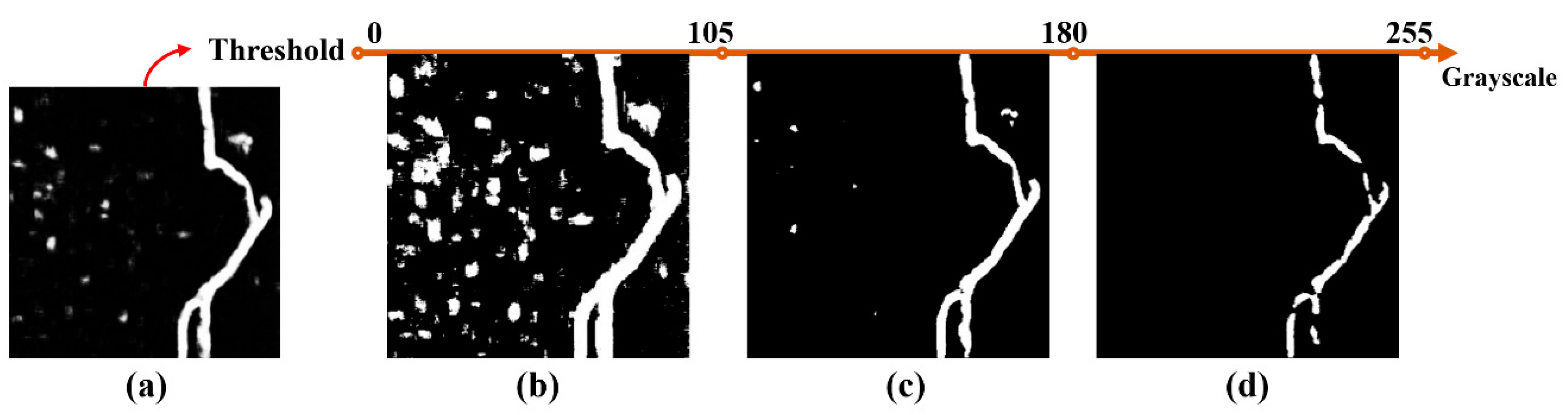
It is important to select the appropriate gray value for threshold segmentation of recognition results [27]. Taking the image recognition of patched pavement crack as an example (Figure 5), the inappropriate gray value can easily yield a considerable difference between the reverse labeled area and the actual area. For example, when the image is segmented by a threshold value in the gray interval of 0–105, Figure 5b, the noise in the segmented image is exposed too much as the gray scale value is too low, which greatly increases the workload of subsequent label modification, i.e., correction labeling. Similarly, it is easy to cause distortion of image details and information loss when the threshold segmentation is carried out in the gray interval of 180–255, Figure 5d. On the contrary, when the image is segmented by a threshold value in the gray interval of 105–180, as shown in Figure 5c, the image retains sufficient boundary and detail information, and the noise in the original recognition result is reduced satisfactorily, which is suitable for reverse labeling.

3.2. Active Correction of Image Recognition Results

The visualization operation of reverse labeling can directly reflect the recognition result of network, while the correction labeling can generate a series of editable points on the boundary of polygon through topological relations, making the image of labeling area editable, as shown in Figure 6. Furthermore, correction labeling can remove the redundant part of image in the reverse labeling, and modify the boundary and other operations. Essentially, the correction labeling is an error correction process for the network, which not only corrects the network recognition errors, but also guides the subsequent sample selection. The images after active correction labeling are merged with those from another original sample set to form a new training set for the next epoch.

As shown in Figure 6, the active correction labeling is able to eliminate the noise points in the upper left corner instead of treating them as a pavement distress patching area. In addition, in the lower right corner, the unrecognized distress is supplemented by added labels. Further, the edge details of some patch areas are adjusted by a series of editing points, and the corrected image labeling are more consistent with the actual geometry of the patched area.

4. Evaluation of Image Prediction Results of Pavement Repair

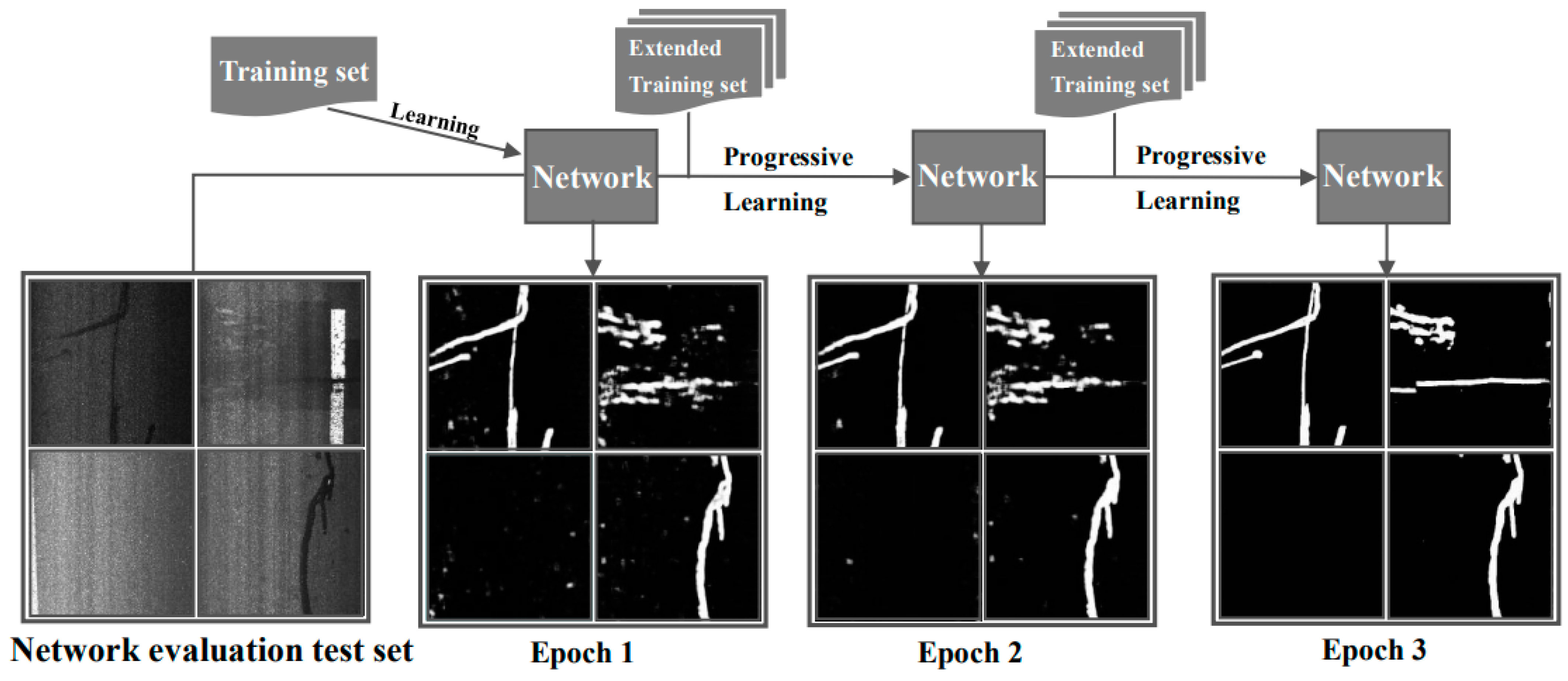
It is important to point out that the sample images through interactive labeling cannot be used as test sets for prediction again. Therefore, it is necessary to reserve a test set with appropriate capacity by random selection for network evaluation (Figure 7). This test set does not participate in interactive labeling, but is only used to compare with prediction results from different epochs of learning process in terms of noise, boundary, and morphology, etc. Meanwhile, the recognition ability of network can be evaluated additionally using the mean_IOU index.

4.1. Boundary Accuracy of Patched Distress

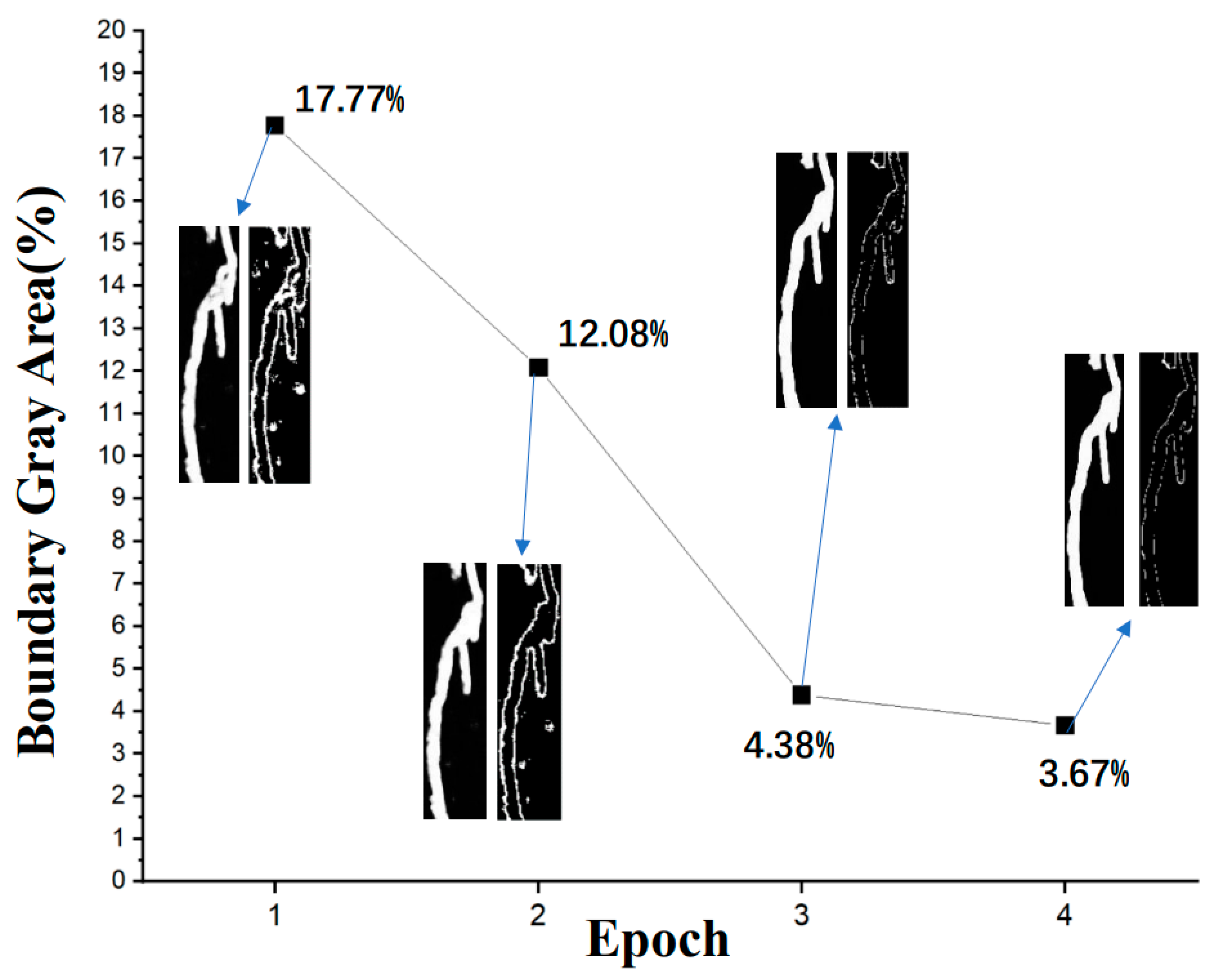
Theoretically, the image gray value of accurately identified pavement distress patched area should be 255, and 0 for other areas. In this study, the region with gray value between 5 and 250 is treated as the fuzzy portion (gray area). The smaller the proportion of gray area, the clearer the boundary of the image. Through calculation, it is found that the boundary fuzzy issue generally exists in the first-epoch recognition results, and the gray area accounts for about 17.77%. The insufficient recognition is attributed to the small sample size (45 images). The boundary definition in the recognition result is improved significantly by increasing the sample size and using the interactive labeling method proposed in this paper. For instance, as shown in Figure 8, through two epochs of interactive labeling and learning, the proportion of boundary gray areas in the recognition results decreases from 17.77% to 12.08% and 4.38%, respectively. For the third epoch, the incremental improvement lowered (the proportion of gray areas is as low as 3.67%), indicating a stabilizing trend. This observation shows that the accuracy of recognition results with the U-Net network can be significantly improved through interactive labeling and learning, which effectively solves the issue of fuzzy boundary.

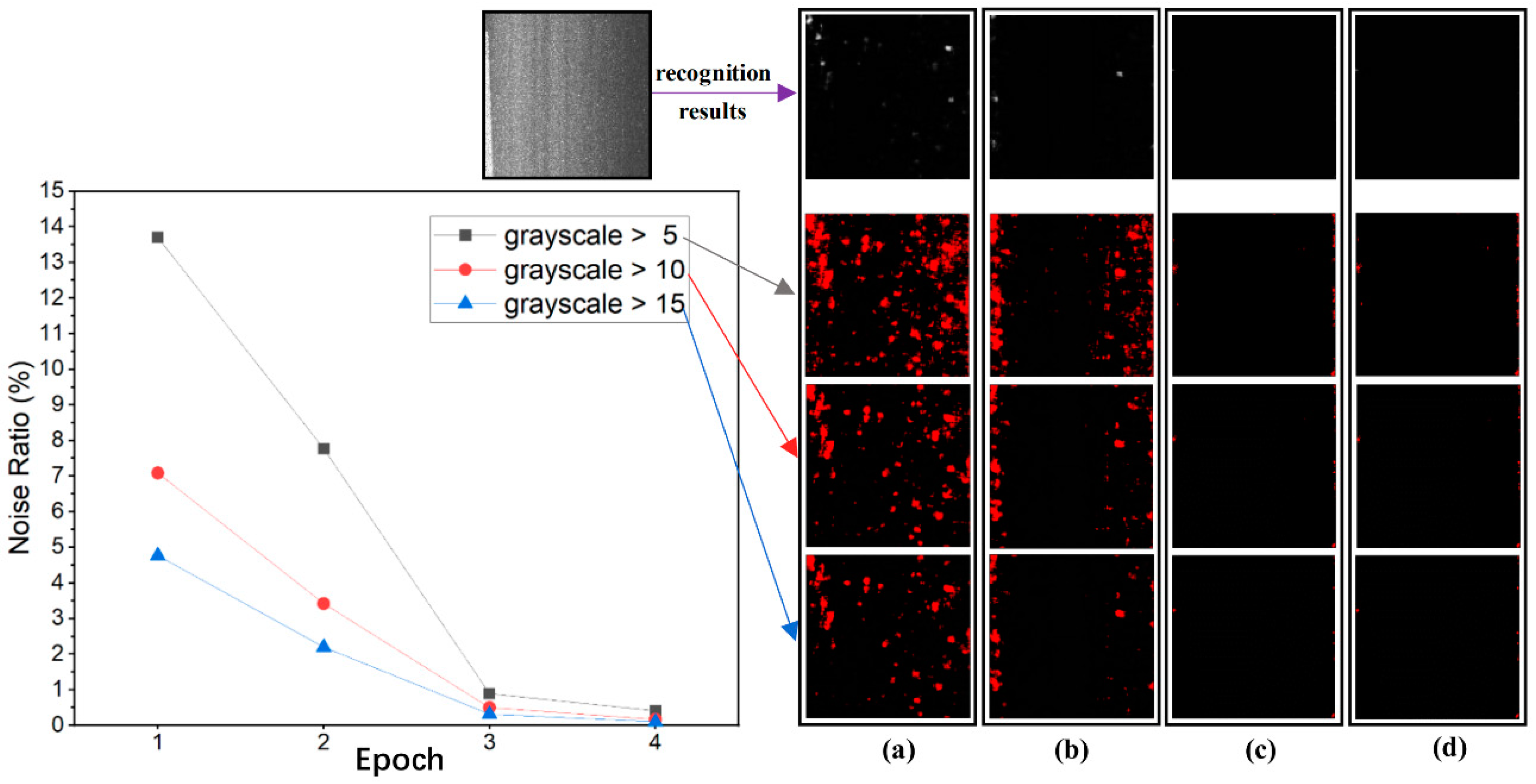
4.2. Image Noise of Recognition Results

In the process of interactive labeling, the images with noise or misidentification are screened, and some noise can be eliminated by appropriately choosing the gray values for threshold segmentation. The remaining noise can be removed by the active correction labeling process. It is thus suggested that attention should be paid to the non-patched area during network learning. The recognition results of noise points are to be verified by distress-free images. Theoretically, the recognition results of distress-free images should all be black with the gray value of 0, and misrecognition would result in color spots (noise) with gray values greater than 0. In this paper, the noise is labeled and analyzed by threshold segmentation with gray values of 5, 10, and 15, respectively, as shown in Figure 9.

It can be seen from the left plot in Figure 9 that the proportion of network recognition noise gradually decreases, and the recognition ability is improved under multiple epochs of interactive labeling and learning process. As shown in Figure 9a–c, the interactive learning of the first two epochs has pronounced effects. For instance, using the gray value of 5 provides an extremely high de-noising performance, while for gray values greater than 5 a reduction rate of 13% is noted during the first two epochs. In the third epoch, the de-noising rate and the proportion of noise are less than 1% and 0.5%, respectively, for gray values of 5 and beyond. The interactive labeling and learning play a significant role in improving error recognition of the U-Net network.

4.3. The Learning Process Based on Interactive Labeling

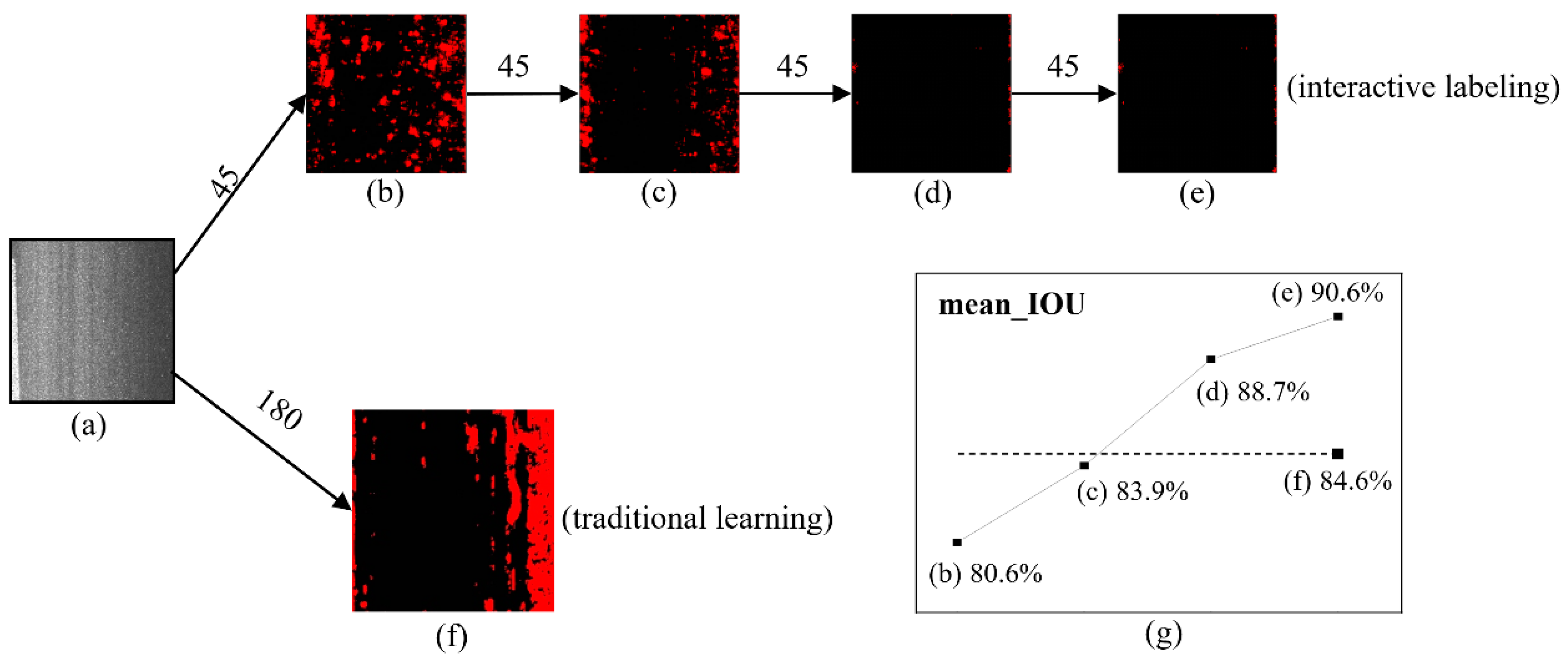
In order to illustrate the benefit of interactive labeling and learning process on the recognition result of pavement distress patching, two typical scenarios are compared in terms of different training set sizes and labeling processes. In Scenario 1, the 180 labeled images are directly fed into the U-Net convolutional neural network model for training and prediction. As a comparison, in Scenario 2 the proposed interactive labeling and learning is applied for image recognition. Specifically, the labeling and learning process is described as follows: after 45 labeled image samples are trained and predicted by U-Net in the first epoch, the recognition images are reversely labeled and actively corrected using the interactive labeling method. Another 45 unlabeled images are then predictively labeled, which are combined with the corrected 45 images to form a new training set for the next epoch of training and prediction. This process is repeated for several epochs until the sample size reaches 180.

For Scenario 1, as shown in Figure 10f, since the misrecognition is not corrected in the learning process, the average ratio of noise points is 16.56%, indicating strong noises with high gray value (about 250–255). In addition, the proportion of gray area of boundary reaches 9.28%, and hence a poor boundary definition. On the contrary, in Scenario 2, as shown in Figure 10a–e, 45 learning sample images are fed into the U-Net, and after three epochs of interactive labeling and learning, a substantially better recognition accuracy is achieved. The accuracy of the U-Net represented by the mean_IOU index reaches 90.6% under the interactive labeling of 135 images in three epochs, compared to 84.6% for 180 sample images, Figure 10g.

In addition, due to the continuous optimization of the network itself, the recognition accuracy in each epoch shows an uptrend, while the number of images that need to be reversely and correctively labeled decreases. This observation contributes to reducing the work in reverse and correction labeling. Compared with the traditional labeling and learning process, the interactive labeling and learning has demonstrated higher efficiency in improving the noise points and boundary definition in image recognition, while requiring a smaller sample size.

5. Concluding Remarks

Image recognition requires a large number of samples for neural network training. Its application to pavement distress patching images generally demands tremendous time and manpower resources for manual screening and labeling. A further complication lies in the subjectivity of labeling personnel, which generally has a great impact on the accuracy of image labeling. In this paper, an interactive image labeling method based on the U-Net convolutional neural network is proposed to deal with these issues and shortcomings. The developed method includes reverse labeling of pavement distress images and active correction of image recognition results.

Reverse labeling helps the labeling personnel find out the shortcomings and errors in the U-Net recognition, and improves the efficiency and accuracy of manual sample correction. Active correction of image recognition results allows the network to actively correct errors, thus improving the accuracy of image recognition. The corrected image set is then merged with the images of the original sample set to form a set with improved quality for the subsequent learning. In order to demonstrate the efficiency and accuracy of the interactive labeling method in image recognition of pavement distress patching, this study compares the recognition accuracy of boundary and image noise between the one-time feed of all samples (180 images) and multiple feeds of 45 images each time.

The following conclusions can be drawn:

(1) The interactive labeling method provides a satisfactory solution to the issues of boundary blur, background noise, misrecognition, and detail loss in image recognition of pavement distress patching, based on the U-Net convolutional neural network.

(2) The recognition ability after interactive labeling is remarkably enhanced after two epochs of network training and tends to stabilize after the third epoch, which demonstrates a much higher efficiency than the one-time feed of all samples for training.

Overall, the proposed interactive labeling method considerably improves the quality of image samples, alleviates the workload of image labeling, and significantly improves the image recognition accuracy. This method is considered suitable for general image recognition applications based on deep learning and is not limited to image recognition of pavement distress patching as a showcase presented herein. The advantage of the method can be shown particularly when the number of samples is small. Implementation of this algorithm in typical image detection systems (e.g., built in inspection vehicles for road condition surveying) is expected to improve efficiency and further promote automation. The findings suggest that the human-computer interaction should be enhanced to take further advantages of computers.

Admittedly, the proposed interactive labeling method still has limitations in practical application. It requires a high labeling accuracy that should be fulfilled by experienced professionals. Additionally, the interactive labeling is not yet fully automated, which is the topic of the follow-up study.

References

- Dan, H.-C.; Wang, Z.; Cao, W.; Liu, J. Fatigue characterization of porous asphalt mixture complicated with moisture damage. Constr. Build. Mater. 2021, 303, 124525. [Google Scholar] [CrossRef]
- Baek, S.-W.; Kim, M.-J.; Suddamalla, U.; Wong, A.; Lee, B.-H.; Kim, J.-H. Real-Time Lane Detection Based on Deep Learning. J. Electr. Eng. Technol. 2022, 17, 655–664. [Google Scholar] [CrossRef]
- Dan, H.-C.; Bai, G.-W.; Zhu, Z.-H. Application of deep learning-based image recognition technology to asphalt–aggregate mixtures: Methodology. Constr. Build. Mater. 2021, 297, 123770. [Google Scholar] [CrossRef]
- Liu, K.; Xu, P.; Wang, F.; You, L.Y.; Zhang, X.C.; Fu, C.L. Assessment of Automatic Induction Self-Healing Treatment Applied to Steel Deck Asphalt Pavement. In Automation in Construction; Elsevier: Amsterdam, The Netherlands, 2021. [Google Scholar] [CrossRef]
- Chen, X.; Pan, L. A Survey of Graph Cuts/Graph Search Based Medical Image Segmentation. IEEE Rev. Biomed. Eng. 2018, 11, 112–124. [Google Scholar] [CrossRef]
- Sezer, A.; Altan, A. Optimization of Deep Learning Model Parameters in Classification of Solder Paste Defects. In Proceedings of the 2021 3rd International Congress on Human-Computer Interaction Optimization and Robotic Applications (HORA), Ankara, Turkey, 11–13 June 2021. [Google Scholar]
- Sezer, A.; Altan, A. Detection of solder paste defects with an optimization-based deep learning model using image processing techniques. Solder. Surf. Mt. Technol. 2021, 33, 291–298. [Google Scholar] [CrossRef]
- Chen, X.; Liu, W.; Thai, T.C.; Castellano, T.; Qiu, Y. Developing a new radiomics-based CT image labeler to detect lymph node metastasis among cervical cancer patients. Comput. Methods Programs Biomed. 2020, 197, 105759. [Google Scholar] [CrossRef] [PubMed]
- Wan, C.; Jin, F.; Qiao, Z.; Zhang, W.; Yuan, Y. Unsupervised active learning with loss prediction. Neural Comput. Appl. 2021. [Google Scholar] [CrossRef]
- Lughofer, E. Single-pass active learning with conflict and ignorance. Evol. Syst. 2012, 3, 251–271. [Google Scholar] [CrossRef]
- Zhang, Q.; Sun, S. Multiple-view multiple-learner active learning. Pattern Recognit. 2010, 43, 3113–3119. [Google Scholar] [CrossRef]
- Chebli, A.; Djebbar, A.; Merouani, H.F.; Lounis, H. Case-Base Maintenance: An Approach Based on Active Semi-Supervised Learning. Int. J. Pattern Recognit. Artif. Intell. 2021, 35, 2151011. [Google Scholar] [CrossRef]
- Qin, J.; Wang, C.; Zou, Q.; Sun, Y.; Chen, B. Active learning with extreme learning machine for online imbalanced multiclass classification. Knowl.-Based Syst. 2021, 231, 107385. [Google Scholar] [CrossRef]
- Liu, H.; Chen, G.; Li, P.; Zhao, P.; Xu, X. Multi-label text classification via joint learning from label embedding and label correlation. Neurocomputing 2021, 460, 385–398. [Google Scholar] [CrossRef]
- Mc Grath, O.; Sarfraz, M.W.; Gupta, A.; Yang, Y.; Aslam, T. Clinical Utility of Artificial Intelligence Algorithms to Enhance Wide-Field Optical Coherence Tomography Angiography Images. J. Imaging 2021, 7, 32. [Google Scholar] [CrossRef] [PubMed]
- Vaiyapuri, T.; Alaskar, H.; Sbai, Z.; Devi, S. GA-based multi-objective optimization technique for medical image denoising in wavelet domain. J. Intell. Fuzzy 2021, 41, 1575–1588. [Google Scholar] [CrossRef]
- Wang, Z.W.; Ding, G.Q.; Yan, G.Z.; Lin, L.M. Adaptive lifting wavelet transform and image denoise. J. Infrared Millim. Waves 2002, 21, 447–450. [Google Scholar]
- Nakashizuka, M.; Kobayashi, K.I.; Ishikawa, T.; Itoi, K. Convex Filter Networks Based on Morphological Filters and their Application to Image Noise and Mask Removal. IEICE Trans. Fundam. Electron. Commun. Comput. Sci. 2017, E100-A, 2238–2247. [Google Scholar] [CrossRef]
- Swami, P.D.; Jain, A. Image denoising by supervised adaptive fusion of decomposed images restored using wave atom, curvelet and wavelet transform. Signal Image Video Process. 2014, 8, 443–459. [Google Scholar] [CrossRef]
- Du, Y.; Pan, N.; Xu, Z.; Deng, F.; Shen, Y.; Kang, H. Pavement distress detection and classification based on YOLO network. International. J. Pavement Eng. 2021, 22, 1659–1672. [Google Scholar] [CrossRef]
- Malini, A.; Priyadharshini, P.; Sabeena, S. An automatic assessment of road condition from aerial imagery using modified VGG architecture in faster-RCNN framework. J. Intell. Fuzzy Syst. 2021, 40, 11411–11422. [Google Scholar] [CrossRef]
- Marsocci, V.; Scardapane, S.; Komodakis, N. MARE: Self-Supervised Multi-Attention REsU-Net for Semantic Segmentation in Remote Sensing. Remote Sens. 2021, 13, 3275. [Google Scholar] [CrossRef]
- Le, J.; Tian, Y.; Mendes, J.; Wilson, B.; Ibrahim, M.; DiBella, E.; Adluru, G. Deep learning for radial SMS myocardial perfusion reconstruction using the 3D residual booster U-Net. Magn. Reson. Imaging 2021, 83, 178–188. [Google Scholar] [CrossRef] [PubMed]
- Han, Y.; Ye, J.C. Framing U-Net via Deep Convolutional Framelets: Application to Sparse-view CT. IEEE Trans. Med. Imaging 2018, 37, 1418–1429. [Google Scholar] [CrossRef] [PubMed] [Green Version]
- Li, Y.; Fang, B.; Zhang, W.; Ding, W.; Yin, J. Deep active learning for object detection. Inf. Sci. 2021, 579, 418–433. [Google Scholar] [CrossRef]
- Barros, W.K.P.; Dias, L.A.; Fernandes, M.A.C. Fully Parallel Implementation of Otsu Automatic Image Thresholding Algorithm on FPGA. Sensors 2021, 21, 4151. [Google Scholar] [CrossRef]
- Liang, Y.; Xu, K.; Zhou, P. Mask Gradient Response-Based Threshold Segmentation for Surface Defect Detection of Milled Aluminum Ingot. Sensors 2020, 20, 4519. [Google Scholar]