Article

Prediction of FRCM–Concrete Bond Strength with Machine Learning Approach

1
AcSIR—Academy of Scientific and Innovative Research, Ghaziabad 201002, India
2
Structural Engineering Department, CSIR—Central Building Research Institute, Roorkee 247667, India
3
Department of Hydro and Renewable Energy, Indian Institute of Technology, Roorkee 247667, India
4
College of Computer Science and Information Technology, University of Anbar, 11, Ramadi 31001, Iraq
5
Department of Civil Engineering, Imperial College London, London SW7 2AZ, UK
6
College of Arts, Media, and Technology, Chiang Mai University, Chiang Mai 50200, Thailand
*
Author to whom correspondence should be addressed.
Sustainability 2022, 14(2), 845; https://doi.org/10.3390/su14020845
Submission received: 24 November 2021 / Revised: 3 January 2022 / Accepted: 8 January 2022 / Published: 12 January 2022

Abstract

:
Fibre-reinforced cement mortar (FRCM) has been widely utilised for the repair and restoration of building structures. The bond strength between FRCM and concrete typically takes precedence over the mechanical parameters. However, the bond behaviour of the FRCM–concrete interface is complex. Due to several failure modes, the prediction of bond strength is difficult to forecast. In this paper, effective machine learning models were employed in order to accurately predict the FRCM–concrete bond strength. This article employed a database of 382 test results available in the literature on single-lap and double-lap shear experiments on FRCM–concrete interfacial bonding. The compressive strength of concrete, width of concrete block, FRCM elastic modulus, thickness of textile layer, textile width, textile bond length, and bond strength of FRCM–concrete interface have been taken into consideration with popular machine learning models. The paper estimates the predictive accuracy of different machine learning models for estimating the FRCM–concrete bond strength and found that the GPR model has the highest accuracy with an R-value of 0.9336 for interfacial bond strength prediction. This study can be utilising in the estimation of bond strength to minimise the experimentation cost in minimum time.

1. Introduction

The necessity for retrofitting existing concrete infrastructure is essential due to ageing, environmental-induced degradation, lack of maintenance, or the need to fulfill current design standards [1]. Developed countries are mainly affected due to the above-mentioned issues, where RC infrastructure components were being used for decades [2,3,4]. The demolition of deteriorated structures is not a sustainable solution, and it is also expensive. To address such kinds of problems and also to increase the capacity (flexure, shear, axial and moment) of structural elements, researchers introduced a new class of composite materials called fibre-reinforced polymer (FRP) [5,6,7,8,9,10,11,12], fibre-reinforced cement mortar (FRCM) [13,14,15,16] or textile-reinforced mortar (TRM) [17,18,19] and textile reinforced concrete (TRC) [20,21,22,23]. In the last two decades, FRP composites have been utilized progressively in construction industry for their high tensile strength and low weight [24]. FRP composites are widely used as an external strengthening material with the use of epoxy resin. However, recent studies show that that FRP has same drawbacks or limitations such as poor performance at elevated temperatures, poor vapour permeability and, sometimes, compatibility issues with concrete or masonry substrate [25]. These limitations restrict the use of FRP.
Various researchers have been suggested that the organic matrices (epoxy resins) can be replaced with inorganic (mortar) matrices to ease the difficulties associated with the usage of epoxies. However, due to the size of the grains in the mortar, the penetration and impregnation of the fibre sheets has been proven to be extremely difficult in this situation; even a thin mortar cannot saturate fibre bundles as resins can [26,27]. Hence, fibre sheets were replaced by the textile material to increase the bond strength conditions. The TRM or TRC materials were introduced initially in Europe and later in the US with the name of FRCM. The textiles utilized as reinforcement are generally long woven, unwoven or knitted rovings produced in at least two orientations (typically orthogonal).
TRM composites have been increasingly used from the last one and a half decades in the repair and rehabilitation industry, as well as in the new prefabricated structural elements. TRMs have a diverse variety of mechanical characteristics due to many types of textile and mortar matrices available. Alkali-resistant glass (ARG) [28,29,30], basalt [31,32,33,34], carbon [35,36,37,38,39], polyphenylene bezobisoxazole (PBO) [40,41] and other natural (e.g., flax [42,43], hemp [44] and sisal [45,46,47]) fibres are the most frequent non-metallic materials used in textiles and can be dried, coated or impregnated into the matrix. Figure 1a–f depict images of textiles made from various fibre materials and geometries. The amount, materials and spacing between rovings in both orthogonal directions may be adjusted independently, resulting in textiles with varied geometries and materials in both orthogonal directions. In order to increase bond quality, these fibres are generally organized in bundles, and their configuration can be changed from unidirectional to bidirectional textile. The various advantages of TRM includes fire resistance, ease of application, low cost and good compatibility with concrete and masonry substrate.
The bond between TRM and the concrete substrate plays an important role in the strengthening procedure and effectiveness. The connection between the reinforcing material and the concrete substrate determines how efficient external strengthening systems are at transmitting stresses. A bond is used to transfer forces from the reinforcement to the mortar. The geometry of roving, surface condition (dry or wet), degree of impregnation and surface preparation are the key parameters which affect TRM–concrete bond strength. In case of fire, TRM performs better compared to FRP because the of breathability and non-flammability offered by cement mortar as an adhesive material. Commonly, single and double shear tests are used to investigate the TRM-concrete bond strength.
Only limited analytical models are available in the literature to predict the FRCM–concrete bond strength. Jung et al. [48] provided the bond strength prediction formula, which is a modification of the FRP–concrete bond strength formula. The foundation of these models are based on a specific database, therefore the model can predict the bond strength for that database only. Furthermore, these models used various assumptions to represent the complicated nonlinear connection between bond strength and crucial key parameters during the theoretical deduction process, which decreases the model efficiency. The development of an accurate and computationally efficient prediction technique for FRCM textile bond strength has become necessary.
One such approach would be to use soft computing such as machine learning (ML) techniques. As a prominent domain of artificial intelligence (AI), ML applications have been investigated in a variety of civil engineering areas for the prediction, optimisation and categorisation.
Chen et al. [49] used a gradient-boosted regression trees (GBRT) ensemble leaning algorithm to predict FRP–concrete bond strength. The elastic modulus of fibres, the tensile strength of fibres, the thickness of fabric material, the width of the fibre bonding length, the compressive strength of concrete and the width of concrete block were the input parameters, and the debonding force was considered as the output parameter. The coefficient of determination for the training and testing data were 0.9627 and 0.9269, respectively. The ANN and SVM models were also adopted to compare the results of performance indices. The R-square value of the SVM and ANN models were 0.9151 and 0.8998, respectively. The GBRT method performs with 3.86% higher accuracy than the SVM model and has 5.46% higher accuracy than ANN model.
Basaran et al. [50] utilized the machine learning algorithms to forecast the FRP–concrete bond strength. Five ML models, GPR, ANN, SVMR, regression tress and MLR models, were used to predict the FRP–concrete bond strength, and it was found that the GPR approach has the best accuracy, with a mean value of 0.95 and at standard deviation of 0.14. Baghaei and Hadigheh [51] explored the durability analysis of FRP–concrete bond strength with data-driven machine learning models. The SVM, ANN and decision tree were used to forecast the FRP bond strength and found that, among these models, the ANN model performs best. Su et al. [52] used ANN, MLR and SVM algorithms to predict the interfacial bond strength between FRP and concrete. The input and output parameters used in this study were similar to Chen et al. [49]. In terms of accuracy and efficiency, the SVM-ML technique performs best for predicting interfacial bond strength.
Wang et al. [53] studied the FRP–concrete bond strength behaviour with machine learning algorithms and code formulations. An ANN was optimized with two hybridized algorithms: (i) genetic algorithm (GA) and (ii) particle swarm optimization (PSO). The test results showed that both GA-ANN and PSO-ANN models performs better compared to the traditional ANN model. Because of its unique information-sharing method, the PSO-ANN beats the GA-ANN when it comes to convergence speed and prediction error. Sun et al. [54] explained the multi-objective optimization of a graphite-slag conductive composite applied a SVR (support vector regression) based model. The correlation coefficient achieved was approximately 0.981 on the test datasets with higher accuracy.
Abuodeh et al. [55] used machine learning techniques to predict the shear strength of FRP-strengthened beams. Within the verified resilient back-propagating neural network, the recursive feature elimination method and neural interpretation diagram were utilized to determine the factors that strongly impact the prediction of FRP shear capacity. The findings showed that the resilient back-propagating neural network with the specified parameters was better at predicting FRP shear capacity ( R 2 = 0.885) than the RBPNN with all original 15 parameters ( R 2 = 0.668) when compared to conventional models such as fib14, ACI 440.R-17, and CNRDT200.
Nikoo et al. [56] used a hybrid approach called bat algorithm-ANN to predict the shear strength of FRP-reinforced RC beams. The application was defined using a total of six characteristics relevant to both concrete and FRP properties. The R 2 values obtained by the ANN-BA, ANN-PSO and ANN-GA prediction models were 96.7%, 93.8% and 91.5%, respectively based on the performance indices, it was found that the ANN-BA model performs the best.
Alam et al. [57] developed a machine leaning prediction model to analyze the shear capacity of FRP-strengthened RC beams using Bayesian optimisation algorithm-support vector regression. The results found that the correlation coefficient (R) and fractional bias (FB) were determined as 0.977 and 0.0033, respectively, which are approximately near to 1 and 0, suggesting that the prediction is accurate enough.
Hybrid ensemble machine leaning models were used by Chou et al. [58] to predict the shear strength of RC beams. To increase the prediction accuracy of the model, a smart firefly algorithm (SFA) was used to optimize least squares support vector regression (LSSVR). The use of this model decreases the application’s complexity and eliminated the requirement for computationally expensive modelling.
Fu et al. [59] proposed a time-dependent machine learning model to predict the shear strength of corroded RC strengthened beams. Gradient boosting regression tree (GBRT) algorithm was applied on the 158 shear tests of corroded RC beams. Geometric dimensions, material qualities, reinforcing details and the amount of corrosion were considered as input parameters while shear strength was considered as an output parameter. The developed model makes good predictions, with an R 2 value of 0.9.
The FRP–concrete bond strength was evaluated by Juncheng et al. [60] using machine learning methods. The methodologies used were artificial bee colony (ABC)-ANNN and imperialist competitive algorithm (ICA)-ANN and found that the ICA-ANN model performed better than the ABC-ANN model.
The interfacial law parameters of FRP strips externally bonded to concrete examined by Su et al. [61] using ANN methods. According to the database of load–displacement responses generated from the FE model, the trained ANN model can accurately and concurrently identify the cohesive law parameters.
Machine learning assessment work was conducted by Naser et al. [62] to predict the strength of FRP strengthened RC members. An optimized ANN with genetic algorithms was used to develop a bond–slip model and identify probable failure modes in FRP-strengthened structures. The proposed bond–slip strength prediction model was compared to five existing empirical models, with the optimized ANN-GA model outperforming them all.
He et al. [63] studied the comparison of different machine learning models for the assessment of delamination in FRP composite beams. BPANN, ELM, and SVM models were used as inverse algorithms for assessing delamination parameters, with a focus on interface prediction. Among these proposed models, the SVM-based model outperforms.
Almustafa and Nehdi [64] studied the structural response of FRP-retrofitted RC slabs subjected to blast loading with machine leaning. Gaussian process regression (GPR) and the Gaussian process regression synthetic (GPR-syn) model were used. GPR and GPR-syn had coefficients of determination of 0.9246 and 0.941, respectively. According to statistical performance criteria such as R 2 , MAE and MAPE, the constructed GPR-syn model produced improved predictions as compared to GPR.
A self-tuning machine learning model was proposed by Alwanas et al. [65] to simulate the load-carrying capacity and failure modes of beam–column joint connection. A newly introduced intelligence model called ELM was applied on the 153 experimental datasets. The input features included different dimensions of data from the beam–column junction and concrete specifications, which were constructed to be given for the prediction model. The suggested self-tuning predictive model was evaluated against the multivariate adaptive regression spline (MARS) model, which is a widely used regression model. In comparison to the MARS model, the findings showed that the ELM model had a more accurate prediction performance with an RMSE 18.63 and 14.44, respectively.
Pajand et al. [66] used machine leaning models to predict the crack spacing in the FRP-strengthened RC beams with lap-spliced bars. The flexural crack spacing is predicted using four machine learning models: an adaptive neuro-fuzzy inference system (ANFIS), multilayer perceptron (MLP) neural network, SVR and least mean squares regression. MLP and ANFIS models had better performance than other models.
A gene expression programming (GEP) approach was used by Nguyena et al. [67] to predict the deflection of FRP-strengthened beams. The work trained GEP using a database developed by calculating the effective moment of inertia of 108 constructed beams using 10 equations taken from the literature, taking into consideration the benefits of both theoretical and empirical models. The deflection of FRP-reinforced beams may be predicted with 99% accuracy using a GEP-based model.
The feasibility and reliability of machine learning models such as GPR, SVM, ANN, DT, linear regression and ensemble trees in predicting FRCM–concrete bond strength were studied in this work. For the first time, an experimental database containing 382 unique records of single and double-lap shear tests, as well as 8 characteristics, was gathered and processed for this purpose. In the literature, there is no computer-based model available for predicting the bond strength of the FRCM system. Following that, the framework of the hybrid modelling technique and data processing approach used in this study has been described. The prediction performance of ML models have been evaluated and analysed.
The rest of the paper is organised as follows: Section 2 contains the laboratory methods of bond strength determination. In Section 3, the research significance of this research article has been discussed. Section 4 is about the experimental data collection from the literature and description of the machine learning models. The findings of the prediction models and comparisons with experimental datasets are presented in Section 5. The outcomes of this study have been briefly discussed in the last Section 6 of this article.

2. FRCM–Concrete Bond Test

A variety of established in situ techniques of reinforcing structures with TRM-textiles exist as a result of inspecting the concrete surface and determining the parameters required for strengthening. Premature TRM debonding, on the other hand, is still a key impediment to efficient TRM-textile usage. This might occur as a result of the reinforced structures being exposed to unfavourable environmental conditions in the future. Premature debonding might also occur as a result of unanticipated changes in load patterns that were not taken into account during the strengthening process. The current research direction on building dependable bond models to anticipate debonding in order to overcome this issue. However, due to the related costs, construction time and small quantity of data obtained after the excessive work, the characterisation experiments required to create such bond models on full-scale buildings are not practical. As a result of these variables, more well-designed TRM textile–concrete bond tests in the laboratory are required, particularly for parametric research and quality control.

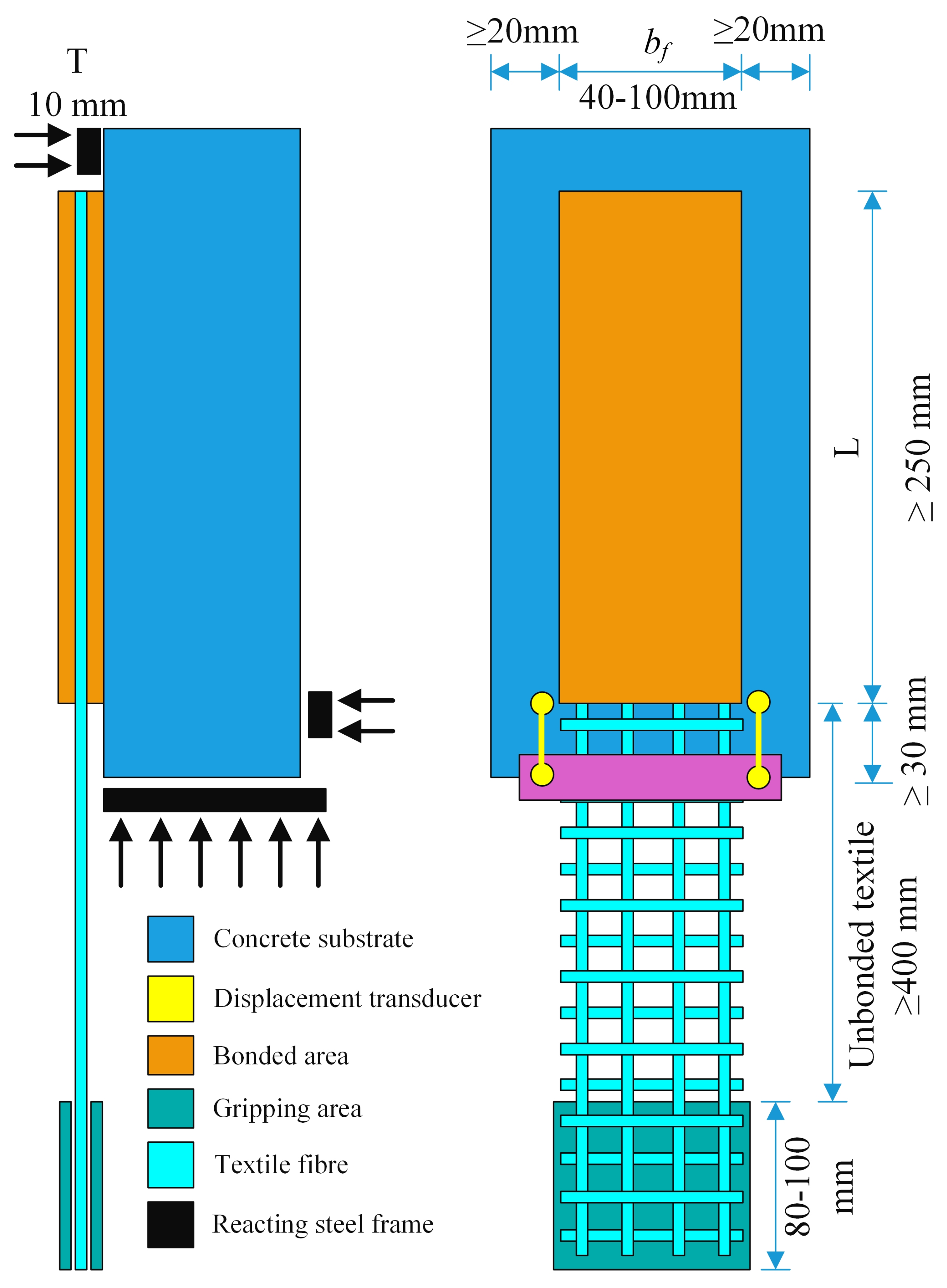
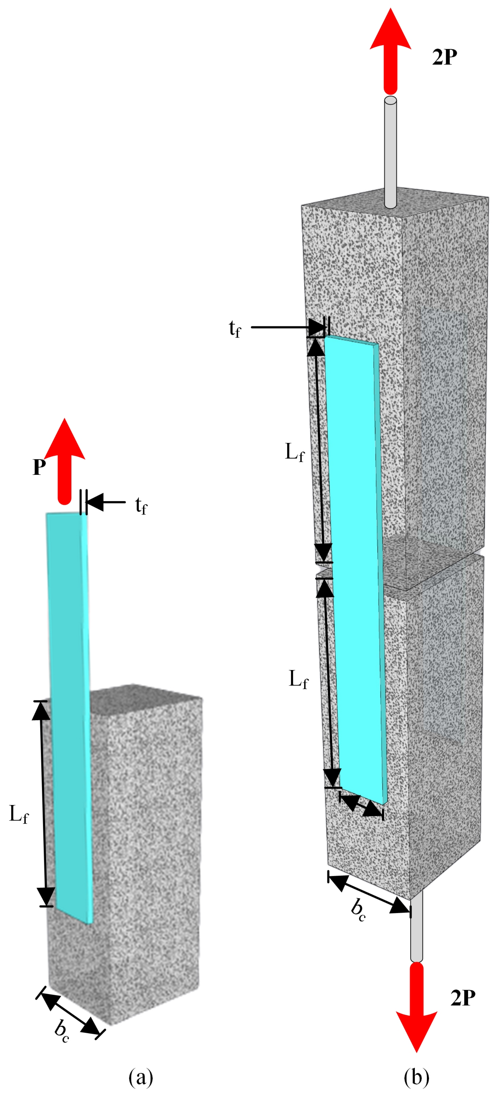
2.1. Single-Shear Lap Test

In this test, a tensile force is applied to a concrete block via TRM fibres attached to one side of the block, as depicted in Figure 2 and Figure 3a. TRM fibres are adhered to the concrete surface with the use of suitable mortar paste. Before applying the adhesive, the surface of the concrete is prepared by eliminating the loose layer of mortar from the concrete substrate using suitable methods such as sand blasting, grinding, water jet, etc. To prevent wedge type of failure in the concrete block, the FRCM textiles are normally left unbonded from the end of the specimen to the inner direction of the specimen. To maximize the potential of TRM textiles, the bonded part must meet the requirement of effective length. Specimens are mounted on steel plates and fastened with bolts throughout the testing process. At the end, the projected TRM fabric is attached to the jaw of testing machine, and the load is applied in a controlled displacement manner. It is the most commonly used method and adopted by various researchers [68,69,70]. The RILEM guidelines for FRCM bond characterization [71] is shown in Figure 2.

2.2. Double-Shear Lap Test

This approach involves concurrently applying tensile force to two TRM textiles bonded on opposing sides of two serially stacked concrete blocks as shown in Figure 3b. The concrete surface roughness and FRCM adhering procedures are the same as for the single lap test. A steel rod is partially inserted into each concrete block to aid in the application of appropriate force throughout its length. Several studies have utilized this technique, including those by Raoof and Bournas [72], Cao et al. [73] and others.

3. Research Significance

To accurately design and simulate buildings using the FRCM composite system, it is critical to use an accurate and efficient model for forecasting the bond strength of FRCM-concrete. There is no computational model available in the literature to forecast the bond strength of the FRCM system. Very limited analytical models are available in the previous studies. The findings of this study will give researchers an algorithm to estimate bond strength, allowing them to plan less experimental work with a higher level of accuracy.

4. Experimental Database Collection
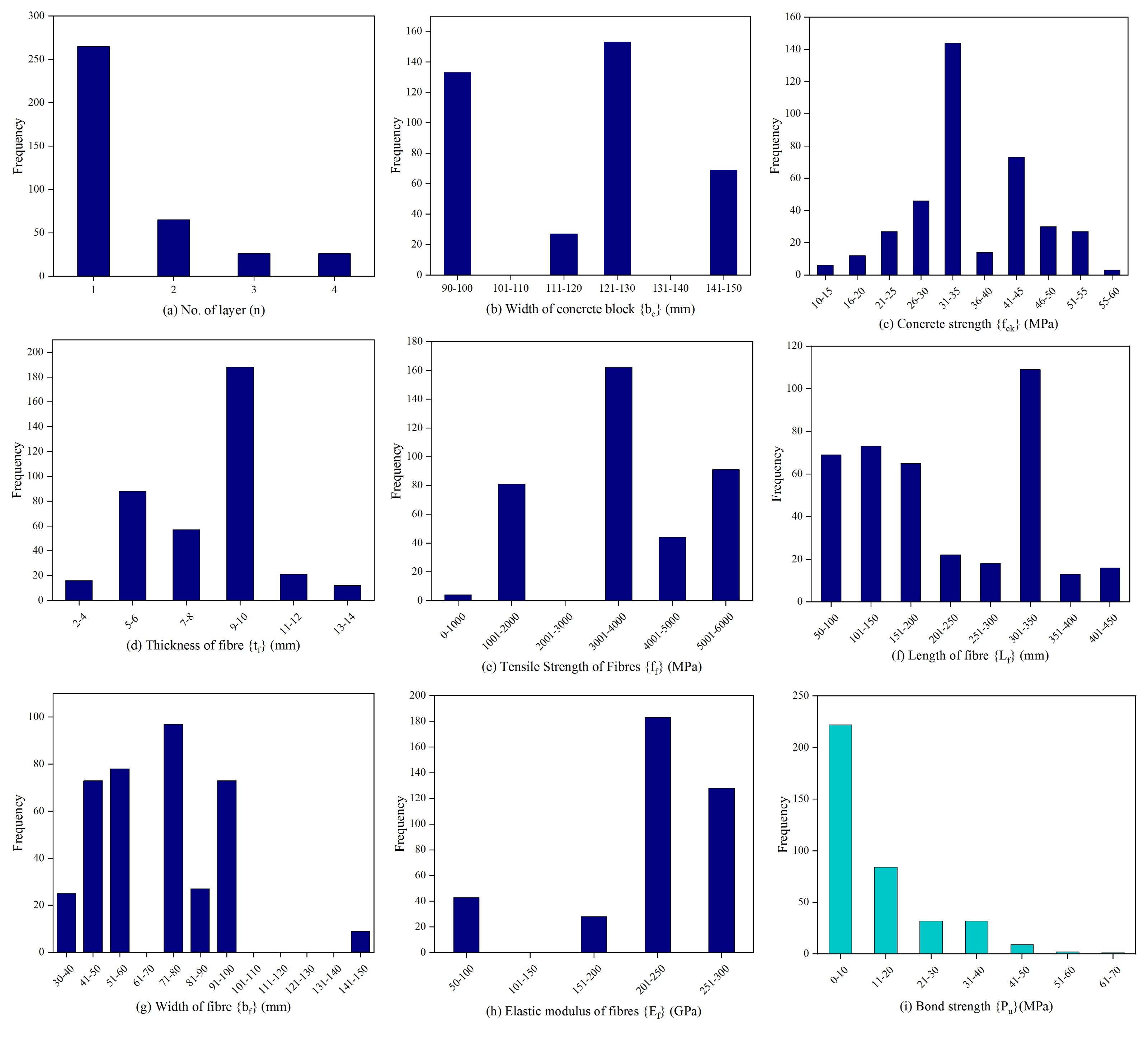
4.1. Database

There is currently no appropriate code for experimental investigations of FRCM–concrete bond strength. The prior studies have only established a few traditional test configurations, such as single shear, double shear, pull-out, pull-off and beam bending tests. Because of its simplicity and efficiency, the single- and double-lap shear tests have become popular in the last decade. As a result, a complete database may be gathered in order to create a data-driven model.
Section 2 explains and illustrates the usual setup of single- and double-lap shear tests. The FRCM concrete compressive stress (f c k ), width of the concrete block (b c ), elastic modulus (E f ), thickness (t f ), tensile strength (f f ), breadth of fabric strip (b f ), bonding length (L f ) and number of layers (n) are all important parameters to consider.
In this work, the database contains the experimental results of 382 single- and double-lap shear tests available in the literature between 2010 and 2021, containing diverse failure modes obtained for examination and assessment of the FRCM–concrete bond forecast model, as shown in Table 1. The FRCM fabric used by researchers in literature contains carbon, glass and polyphenylene bezobisoxazole (PBO). Table 2 shows the statistical features of each major component in the database. Eight input variables have been used to construct different models, which includes six FRCM parameters and two concrete parameters, and the shear force P u was specified as an outcome. The amount of experimental samples in this dataset is more than 10 times the quantity of input variables, ensuring that a data-driven model may be built [74]. The methodology adopted in this work to achieve the objective is presented in Figure 4. In addition, Figure 5 shows the relative frequency distribution of test datasets.

4.2. Performance Indices

The study evaluated the performance of the selected techniques using statistical assessment criteria such as MAE (Mean Absolute Error), MAPE (Root Mean Square Error), R (Pearson Correlation Coefficient) and RMSE (Mean Absolute Percentage Error). Where an R-value closer to 1 suggests a better fitting result, and an R-value more than 0.85 shows a significant connection. The greater the performance of the ML models, the lower the values are of the three indices, MAE, MAPE and RMSE [84]. The related mathematical expressions are expressed in Equations (1)–(5):
R = i = 1 N x i x ¯ y i y ¯ i = 1 N x i x ¯ 2 y i y ¯ 2
where N is the number of experimental datasets, x i is the measured value at ith level, bar x is the mean of measured values, y i is the predicted value at ith level and bar y is the mean of predicted values.
M A E = 1 N i = 1 N E i P i
where E i and P i are the experimental and predicted values, respectively.
MAPE = 1 N l = 1 N E i P i E i × 100
M S E = i = 1 N E i P i 2 N
R M S E = i = 1 N E i P i 2 N

4.3. Pre-Processing of Data

The data were collected from the literature as mentioned in Section 2. All the data were normalized in the range of −1 to +1 using Equation (6). The plotmtrix of the normalized data is shown in Figure 6:
X normalized = 2 × y y min y max y min + 1
In this equation, X n o r m a l i z e d is the final outcome of normalized data, y is the value to be normalized, y m i n is the minimum value in the data set and y m a x is the maximum value in the dataset.
After that, the dataset was divided into two parts on a random basis. A total of 70% of the records were chosen as a training set for the ML models to be trained using supervised leaning. Following that, the remaining 30% of the datasets were utilized as a test set to check the networks performance and assess their generalization capabilities.

4.4. Machine Learning Methods

4.4.1. Linear Regression

Linear regression is a supervised-learning-based machine learning technique. Regression analysis (RA) is a type of statistical examination that is often used to scrutinize the connection between a dependent variable and one or more independent variables. The connection is modelled in order to forecast the future state of the dependent variable. The RA with a single independent variable is known as one-variable or simply called regression analysis (SRA), while an RA using more than one independent variable is known as multiple regression analysis (MRA). Linear regression models are those that are stated by linear equations, whereas nonlinear regression models are those that are not [85]. This information may be acquired by employing the regression line, which is a line that can be computed using Equation (7):
E ( y ) = β o + β 1 x
where E ( y ) is the predicted value of the dependent variable Y, β o is the intercept, β 1 is the regression coefficient and x is a given value of the independent or predictor variable.
MRA is a regression model that estimates the dependent variable based on two or more independent variables that are related to the dependent variable. The independent factors explain the whole variation in the dependent variable. This model may be used to interpret the direction of the relationship between the independent variables and the dependent variable. For a total of n number of independent variables, the mathematical model of MLR analysis is provided in Equation (8):
E ( y ) = β o + β 1 x 1 + β 2 x 2 + β 3 x 3 + β 4 x 4 + + β n x n
where β 1 , β 2 , β 3 , β 4 and β n are the regression coefficients of x 1 , x 2 , x 3 , x 4 and x n , respectively.
When other independent variables are maintained constant in an MLR model, the slopes β i correspond to the increase in the dependent variable E(y) as a consequence of the unit increment in the respective independent variable (x i ) [86].

4.4.2. Regression Tree

In 1984, Leo Breiman proposed regression trees for the first time [87]. As a result, decision tree (DT) learning has sparked a lot of attention. In regression analysis, a case is defined as ( x , y ), where x is the attribute vector and y is the target. A regression function is used to estimate how the goal y changes as x is changed when the connection between x and y is changed. In the proposed approach, all types of regression trees were applied. Three steps are involved in the construction of an RT: (1) tree growth using a learning dataset; (2) tree pruning with a test dataset or cross-validation; and (3) best pruned tree selection.
The concepts of training, validation and test sets, as well as the concerns of over-fitting versus under-fitting, have been applied to DT. A tree in a graph-theoretic sense is the fundamental model in DT learning. However, there is a stylized control flow that is overlaid on the tree structure that must be recognized. A decision-type question is asked at each inner node of the tree, also containing the root. Based on the answer, the next child node will be decided. At last we reach to the leaf node and have classification of the dataset because each leaf node has its class level. DT learning has the benefit of being able to capture more complicated decision boundaries than other learning approaches such as logistic regression. There is no hyperplane that divides samples of two different classes, therefore, DT learning is useful for samples that are not linearly isolated. The capacity of decision trees to represent complicated decision boundaries can be a trap in and of itself, since overfitting can occur unless other approaches, such as “pruning the tree”, are used.
Decision trees are popular due to a few other benefits. To begin with, they frequently result in a clear visual representation of how the ML system conducts categorization. Additionally, the training process is generally quick and can handle huge amount of data. Finally, decision trees are commonly employed in ensemble learning approaches such as AdaBoost and random forests. Bagging is a large category of machine learning algorithms that includes random forests. Overfitting is particularly well-served by bagging methods. Multiple decision trees are learnt in random forests, which are then combined to form a graph-theoretic forest. The various decision trees in the forest categories are based on the new feature vectors. The final classification is created by combining these separate categories.
Each final region is given a value in order to estimate the intended output. The tree may be represented as a function defined by h as given in Equation (9), with R j defined as the disjoint areas allocated to each leaf of the DT:
h ( x ) = j = 1 j b j 1 x R j

4.4.3. Support Vector Machine (SVM)

Support vector machines (SVMs) were created in the 1990s by Vladimir Vapnik and are based on statistical learning theory. An SVM examines the extreme limits and draws the edges, which are commonly referred to as hyperplanes, that divide two classes. Decision limits that are not ideal can cause the new data point to be misclassified. The extreme data points assist in determining the limitations, known as support vectors, and they prefer to disregard the training data points [88].
In classification applications, support vector machines are extensively utilized. The procedure of identifying the function f(x) with the least difference between empirically experimental responses and predictions for all training datasets is referred to as classical regression analysis. In order to obtain a generalized performance, one of the major feature of SVM is to strive to attain the smallest generalized error limit rather than the smallest observed training error. This generalized error limit is defined by a combination of the arrangement term, which limits the complexity of a collection of functions, and the training error.
A training set expressed in the regression process is in Equation (10):
Z = x 1 , y 1 , x 2 , y 2 , , x m , y m
where y m and x m express the dependent and independent variables of the regression models, respectively.
y i = i = 1 n α i β i × x , x i + b
where b is the bias and α i and β i represent Lagrange multipliers. In the nonlinear case, the modified equation with added Kernel function is given by:
y i = i = 1 n α i β i × k x , x i + b
where k ( x , x i ) is the Kernel function. Kernel functions include polynomial, radial basis function and hyperbolic tangent.

4.4.4. Gaussian Process Regression (GPR)

“The Concept of Gaussian processes (GP) is named after Carl Friedrich Gauss since it is based on the Gaussian distribution (normal distribution)”. A GP is an infinite group of random variables with a constant joint Gaussian distribution in any of its finite subsets. A mean function and a covariance function are used to represent a GP [89,90]. The mean function is commonly assumed to be zero since the GP is a linear combination of random variables with a normal distribution. GP can be viewed as a nonlinear function distribution. GP is defined as:
f ( x ) G P μ ( x ) , k x , x
where μ ( x ) = mean, and k ( x , x ) = positive-semi definite kernel function which define the covariance between any two realization of f ( x ) and f ( x ) :
k x , x = cov f ( x ) , f x
The mean is often assumed to be zero, i.e., μ x = 0 , and the kernel has parameters θ , i.e., k ( x , x | θ ) . For any infinite collection of inputs X = ( x 1 , x 2 , , x n ) , the f ( X ) = ( f ( x 1 ) , f ( x 2 ) , , f ( x n ) have joint multivariate Gaussian distribution.
f ( x ) N 0 , K X X ( θ )
where the elements of N-by-N covariance matrix are defined by the kernel function:
K X , X ( θ ) i , j = k x i , x j θ
The covariance function aids in the implicit specification of model properties such as periodicity, smoothness, stationarity and so on. As shown in Equation (17), the fundamental and extensively used GPR is made up of a squared exponential covariance function and simple zero mean:
k x , x = σ f 2 exp r 2
In addition, the value of r is expressed in equation:
r = x x 2 l 2
where, l and σ f are the hyper-parameters and effect the performance of Gaussian Process. σ f denotes the model noise and l is the scale of length. In this paper, all the kernel function rational quadratic, square exponential, matern 5/2 and exponential function are being used. The information and formulation of these function were mentioned in the literature [91,92].

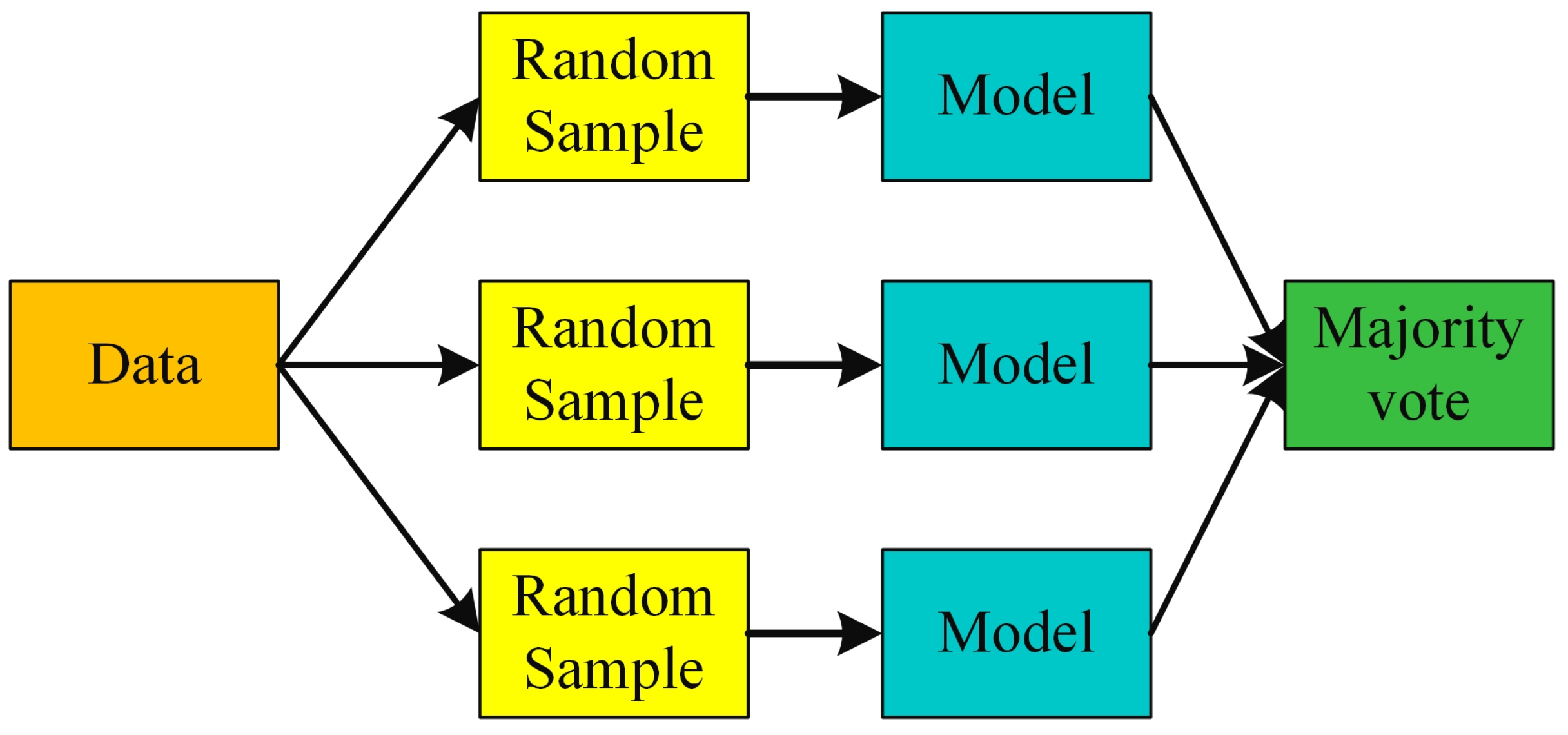
4.4.5. Ensembles of Trees

Several separate trees are joined together to make an ensemble of trees. Despite being one of the most efficient and understandable classification techniques, decision trees have a limited generalization ability. As a result, they have a low bias in the sample but a significant variance out of the sample. Rather than employing a single decision tree, they mix multiple to provide greater prediction results. The ensemble model is based on the idea that a number of weak learners may be united to generate a strong learner. Bagging and boosting are the most common approaches for training ensemble decision tree models [93].
The boosted regression tree (BRT) [94,95] is a hybrid of regression tree and boosting. Many decision trees, such as the random forest model, have been fitted to the BRT multiple times in order to increase the model’s accuracy. There was a distinction between the two approaches utilized to generate the data’s selected trees. In both strategies, all data for the building of each new tree was chosen at random, as shown in Figure 7. The baggage approach was utilized in the random forest model, which revealed that the probability of successive samples being selected for each occurrence was the same. The input data were weighted in the trees, and BRT was employed as a boosting strategy. The weights were inadequately approximated when using this model, resulting in the prior tree being selected as the new tree. This means that the first tree fitted to the model will account for the inaccuracy and will become a new tree. Taking the old tree against a new tree enhanced the model’s accuracy and made it a powerful model. The boosted regression tree considered two parameters such as tree complexity and learning rates.
When we want to minimize the variance of a decision tree, we employ bagging (bootstrap aggregation). The primary idea behind this method is to create various subsets of data from the training sample, which is chosen at random via replacement. Each subset of the data is utilized to train the decision tree model that corresponds to it as presented in Figure 8. As a result, a variety of models emerge. Finally, rather than using a single decision tree, the average of all forecasts from several trees is employed, which is more powerful and accurate.

4.4.6. Artificial Neural Network

Artificial Neural Networks (ANNs), discovered by McCulloch and Pitts, play a critical role in Artificial Intelligence (AI) [96]. Artificial neural networks (ANNs) are sophisticated data processing systems based on the human brain system [97]. ANNs are made up of basic elements (which are also known as nodes or neurons). To build a layer, the neurons must interact with one another and combine. Neurons are linked together via connection links, each of which has a different weight. Every neuron captures a weighted sum of inputs (signal). Each neuron has a unique transfer function (sometimes referred to as the activation function), and the output signal is created when the weighted sum of inputs exceeds a specified threshold. Because the flow of information occurs in the forward direction, this activity is termed feed-forward. Gradient descent and backpropagation are commonly employed to decrease error (the difference between output and goal variables). The suggested network design is depicted in a simplified form in Figure 9. This proposed ANN model has three hidden layers. The Levenberg–Marquardt backpropagation algorithm was used to train the model. The capacity of ANN to learn is a key aspect in forecasting bond strength. A collection of input/output data can be used by ANN to build a non-linear structure [98]. ANN has been successfully employed by several studies to forecast the strength of the FRP–concrete connection [99,100].
Each neuron receives inputs from the top layer, calculates the weighted total of those inputs and uses an activation function to create outputs for the next layer. The set of inputs X = ( x 1 , x 2 , , x n ) will be multiplied by the weight vector W j = ( w j 1 , w j 2 , , w j n ) . Lastly, the biases are added into it as shown in the following equation:
Y j = i = 1 n w j i x i + b j
where Y j is the weighted sum of outputs.

5. Results and Discussion

It is common to evaluate the model performance once a predictive approach has been fully constructed.The analytical estimates produced from the ANN, regression tree, GPR, linear regression, SVM, ensemble tree, optimized GPR, optimized SVM, optimized ensemble tree and optimized regression tree machine learning algorithms are presented in this section. To evaluate the performance of each algorithm, the statistical assessment criteria R, RMSE, MAPE and MAE were used. The calculation process was carried out on a Desktop Intel(R) Core (TM) i5-4570 CPU @3.20 GHz, 8 GB RAM.
It has been found that in linear regression model, the best achieved algorithm was interactions linear with an off robust option. The R-value of this model is 0.9284, which is 0.55% lower than the GPR model. Similarly, in regression trees, the best fitted model was a fine tree with a minimum leaf size of four. In this model, the (regression coefficient) R-value is 0.9102, which is 2.51% less than the GPR model. The other performance indices such as RMSE, MAPE and MAE have values of 4.6527, 26.1715 and 2.6228, respectively. In SVM, the quadratic SVM is the best-fitted model with automatic box constant mode. The overall R-value of SVM is 0.9239, which is 1.04% lower than the GPR model values. GPR and ensemble-boosted tree are the best-fitted models, having overall R-values of 0.9336 and 0.9102, respectively. Figure 10 compares the predicted values of all machine learning methods.
Table 3 shows the results of a number of statistical measures derived from various models in order to analyze their performance quantitatively. The performance metrics R, RMSE, MAPE and MAE for the GPR model are 0.9435, 3.6443, 24.2188 and 2.0179 on the training data, and 0.9130, 4.7904, 23.8626 and 2.7193 on the test data, respectively, as shown in Figure 11. The R-value for test data is 3.2326 % lower than for training data, and the RMSE and MAE for the test data are 31.45% and 34.76% higher, respectively. For the training data, it was indicated that the GPR model may overfit the data when predicting the FRCM–concrete bond strength. However, the value of the MAPE testing set is decreased by 1.4927 % compared to the training data.
The performance metrics R, RMSE, MAPE and MAE for the ANN model are 0.9538, 3.2951, 18.3171 and 1.5887 on the training data and 0.8871, 5.4525, 22.8626 and 2.8801 on the test data, respectively. The R-value for test data is 6.99% lower than for the training data, and the RMSE, MAPE and MAE for test data are 65.47%, 24.82% and 81.28% higher, respectively. For the training data, it was indicated that the ANN model may overfit the data when predicting the FRCM–concrete bond strength. Despite the fact that the statistical metrics of the ANN and GPR models on the training data do not differ much, the overall performance of the ANN model is significantly better than the other models.
On the basis of performance indices, the best fitted models are ANN and GPR. The worst models are regression trees, ensemble boosted trees and optimized regression trees. There is no variation in the performance indices of GPR and the optimized GPR models. The R-value of the improved SVM model is 0.39% higher than that of the SVM model. Similarly, the R-value of the improved ensemble boosted tree is 1.18% higher than that of the ensemble boosted tree model. However, when compared to the regression tree model, the value of the optimized regression tree model increases significantly. Figure 12 presents the variation of experimental data and machine learning models data with respect to data order. The R, RMSE, MAPE and MAE comparison of best prediction models optimized GPR, GPR and ANN is shown in Figure 11.
Figure 13 shows the experimental and predicted bond strength calculated by the ANN, ensemble tree, GPR, linear regression, regression tree and SVM. Figure 14 shows the experimental and predicted bond strength calculated by optimized GPR, optimized regression tree, optimized SVM and optimized ensemble tree. Figure 13 and Figure 14 are used to analyze the error between experimental and predicted values. To speculate the pattern of experimental data, different standard models have been used and compared to predict the variation between experimental data with standard models. The higher variation between experimental data and standard models reflect higher errors. The blue lines in each figure represent the experimental values, while the dotted pink lines are the predicted values. The maroon circles below these values corresponds to their errors.
In comparison to other models, the bond strength dataset produced from the GPR, the optimized GPR and ANN models give the maximum precise results and extremely matched to perfect fit line, as shown in Figure 10a,c,h. Figure 15 also shows the distribution of absolute error values, which may be used directly to compare the error value ranges with all ML models. When compared to other models, the absolute error datasets for the GPR, optimized GPR and ANN models are focused in the lower circle range. As a result, the GPR, optimized GPR and ANN model performs well with other techniques and has the greatest precision and resilience. Additionally, the absolute error datasets of GPR, optimized GPR and ANN lie in often less than 8 kN error range (about 97.07%, 96.97% and 96.43%, respectively).

6. Conclusions

Various machine learning techniques are used to evaluate the bond strength between FRCM composites and concrete substrate. Experimental datasets are gathered from the literature, which includes 382 single- and double-lap shear experimental data. Collected data were scaled and normalized in the range of −1 to +1 to better visualize the variation effect. The number of FRCM layers, the compressive strength of the concrete block, the width of the concrete block, the tensile strength, the elastic modulus, the thickness of the FRCM plate and the concrete block width were considered as input parameters to predict FRCM–concrete bond strength. The performance parameters R, RMSE, MAPE and MAE were used to evaluate the performance of the ANN, GPR, SVM, linear regression, regression tree, ensemble learning, optimized SVM, optimized GPR, optimized regression tree and optimal ensemble learning models. The findings revealed that the GPR, optimized GPR and ANN are the best-fitted models for estimating FRCM–concrete bond strength.The following are the quantitative outcomes of this study:
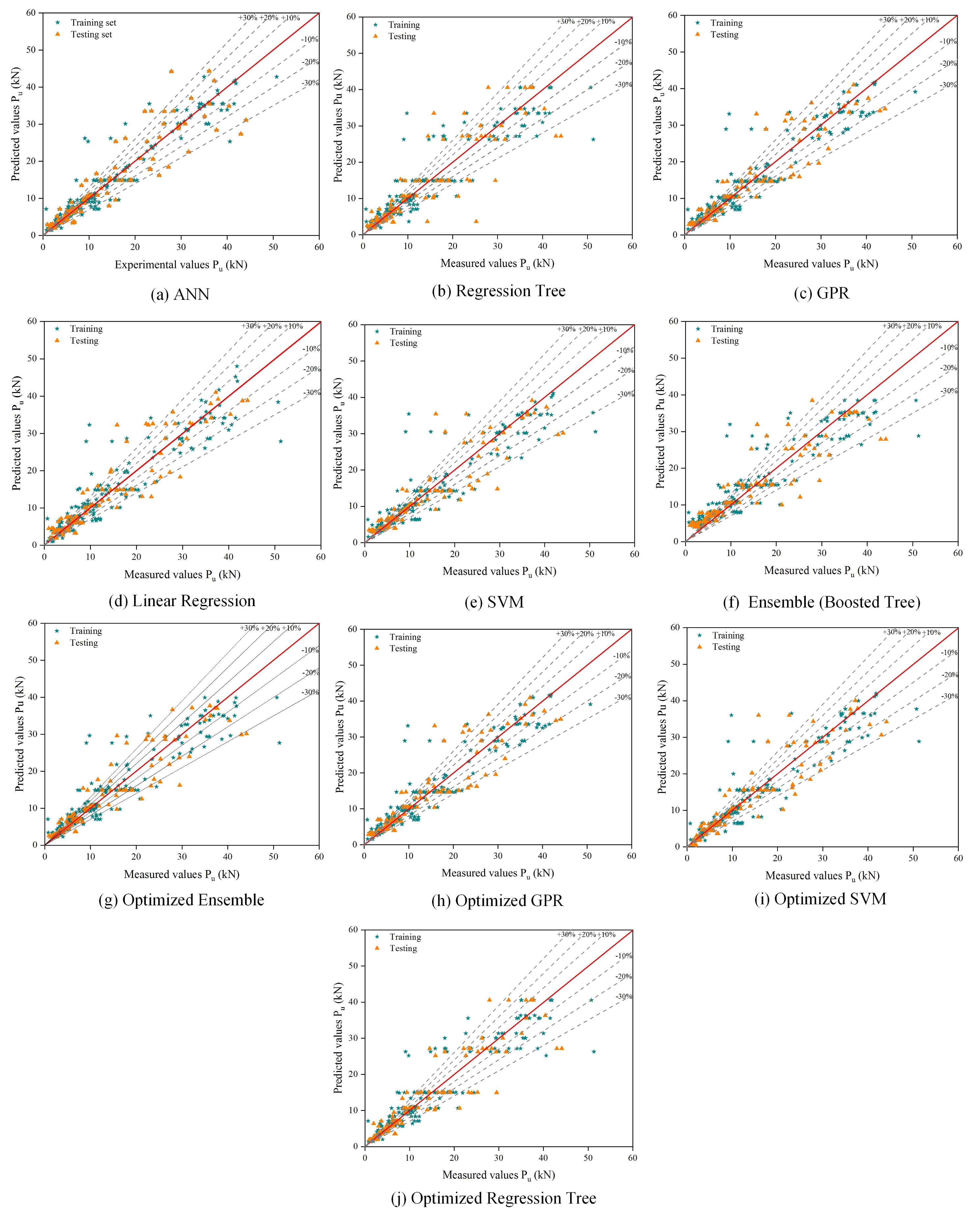
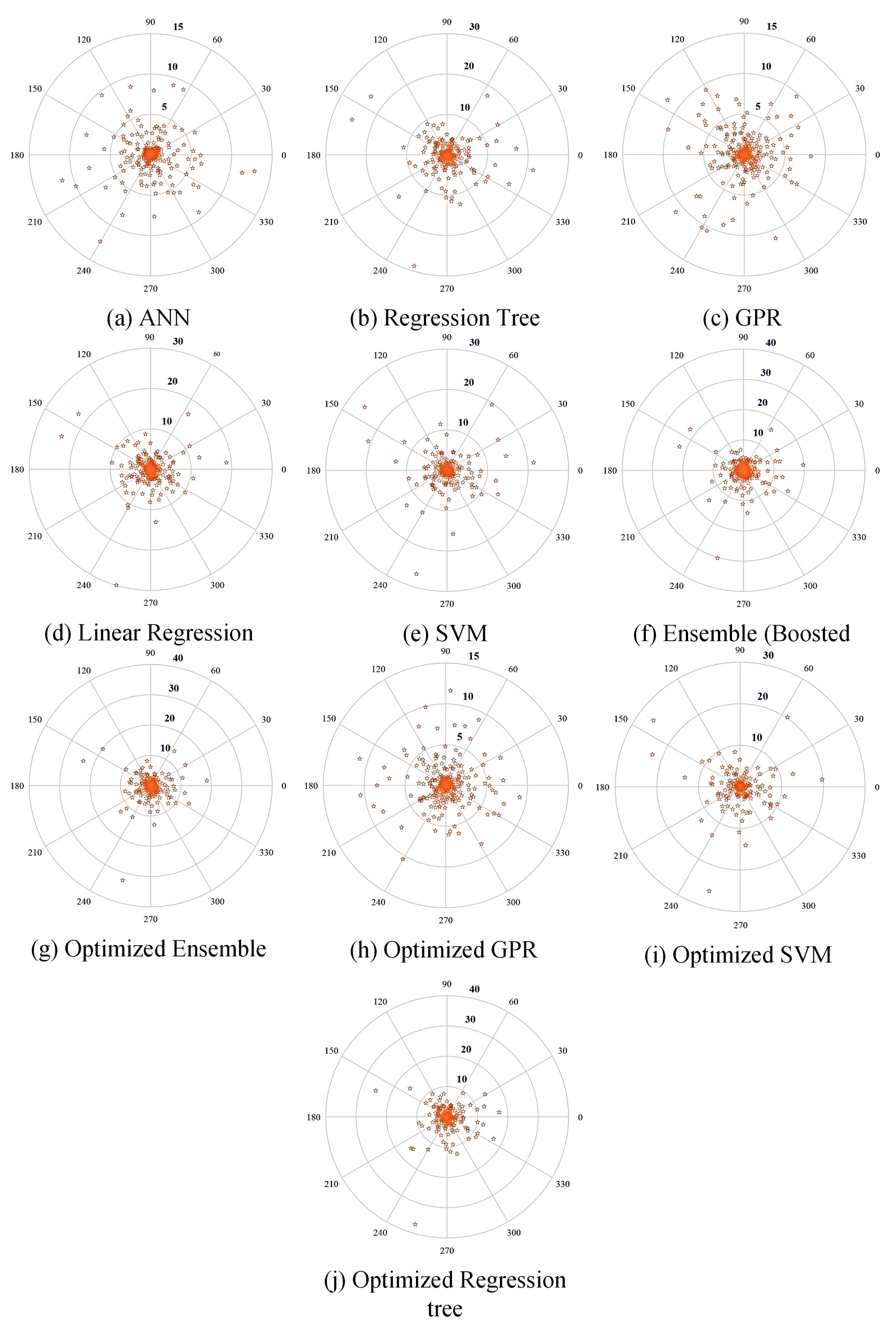
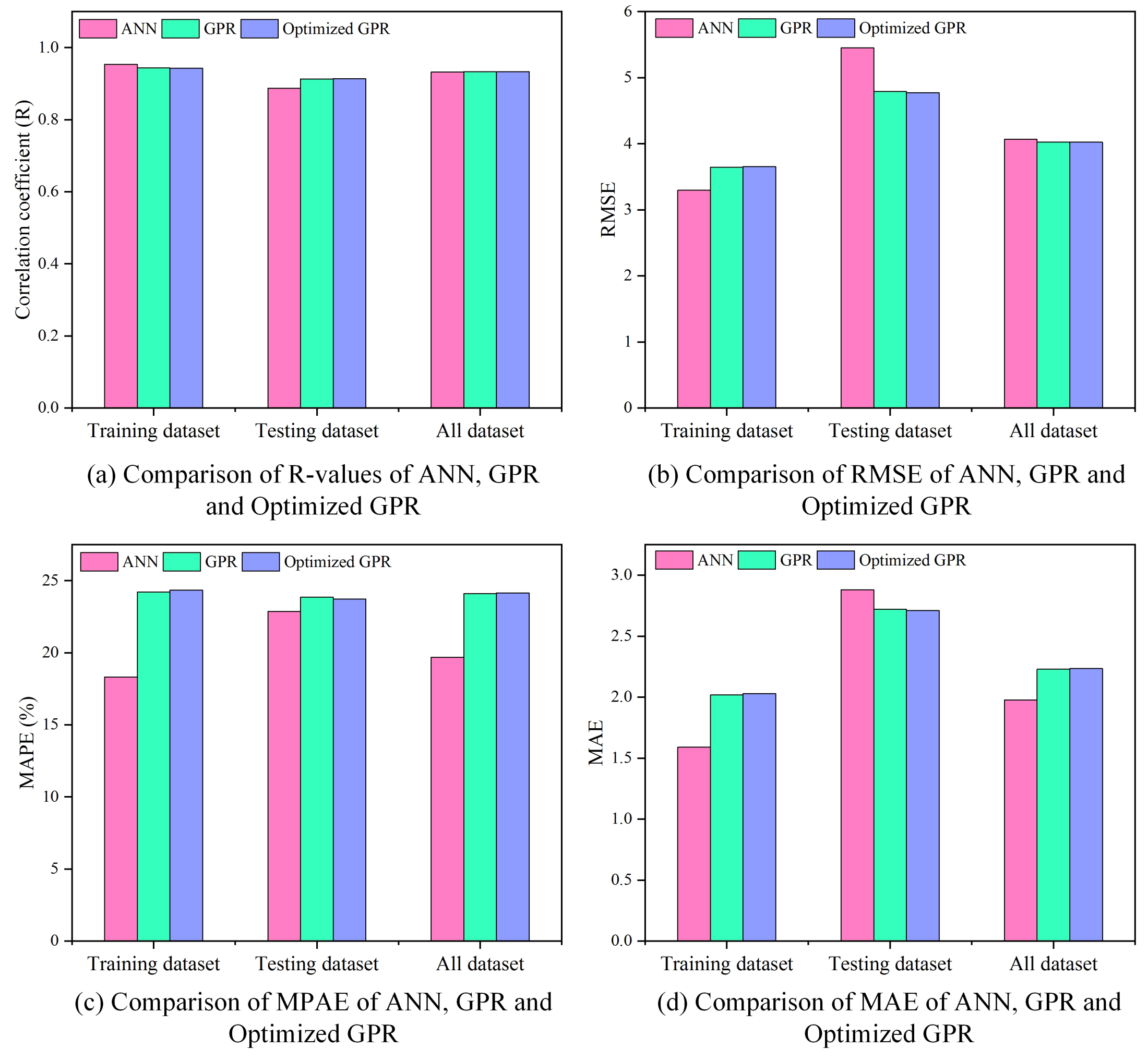
  • The GPR and optimized GPR model can accurately predict the bond strength with R-value 0.9435 and 0.9310 (for training) and 0.9432 and 0.9137 (for testing), respectively.
  • ANN model founds third best fitted model to predict the bond strength with R-value 0.8871 for training and 0.9538 for testing.
  • According to the R, RMSE, MAE and MAPE assessment standards, the precision of the analytical approximations of the optimized GPR, GPR, ANN, optimized ensemble, linear regression, optimized SVM, SVM, ensemble, optimal regression tree and regression tree decreases subsequently.
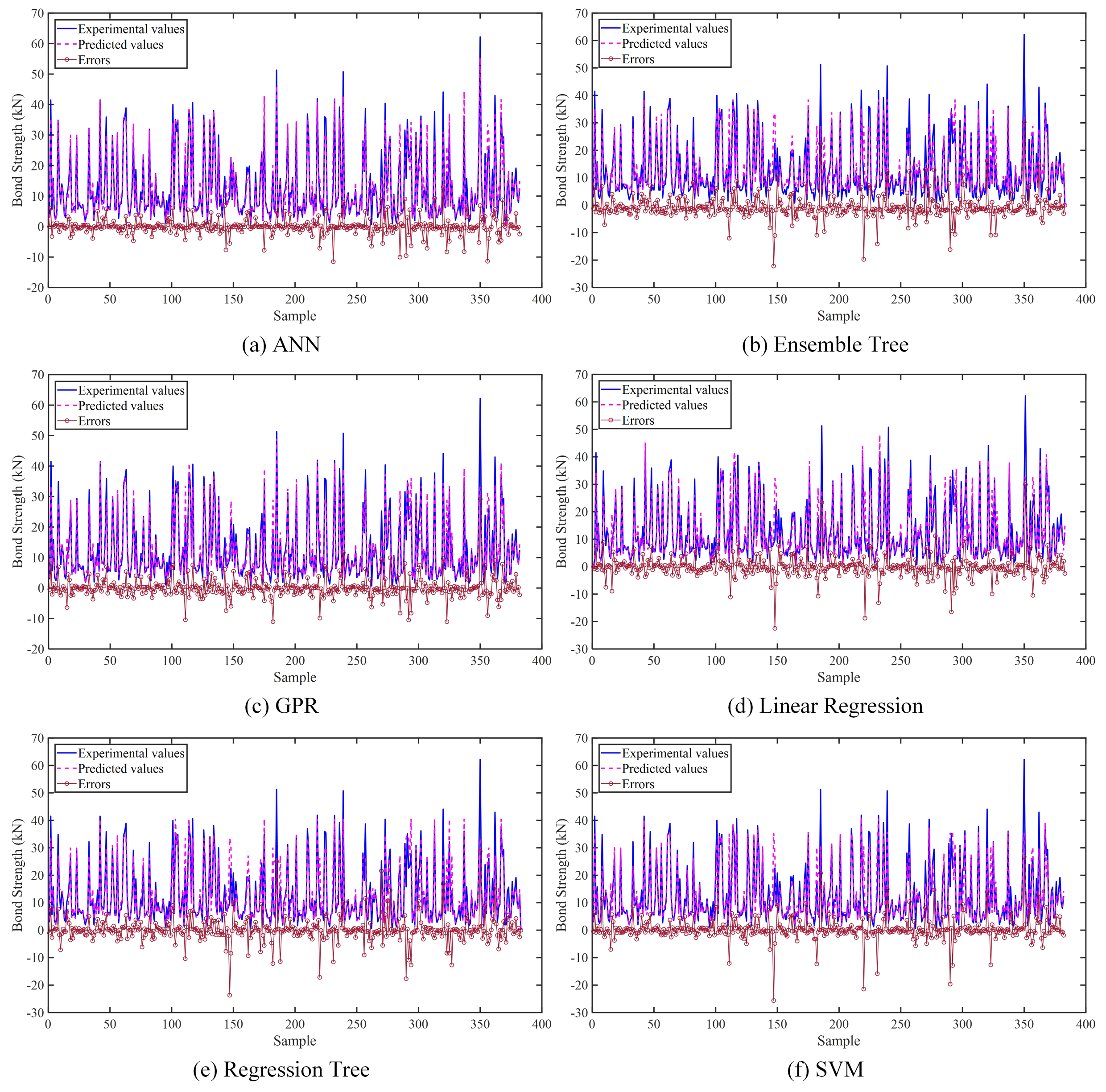
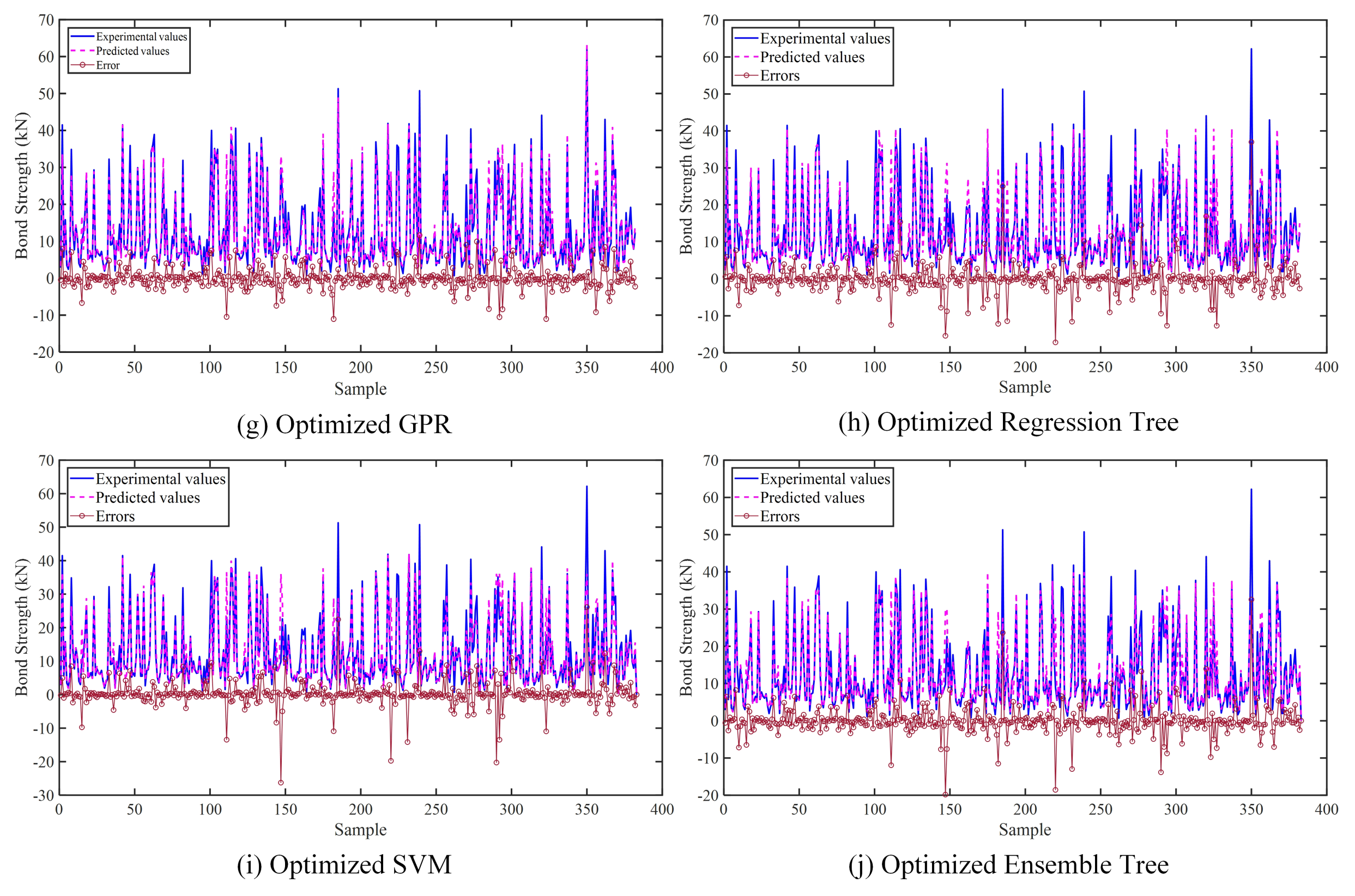
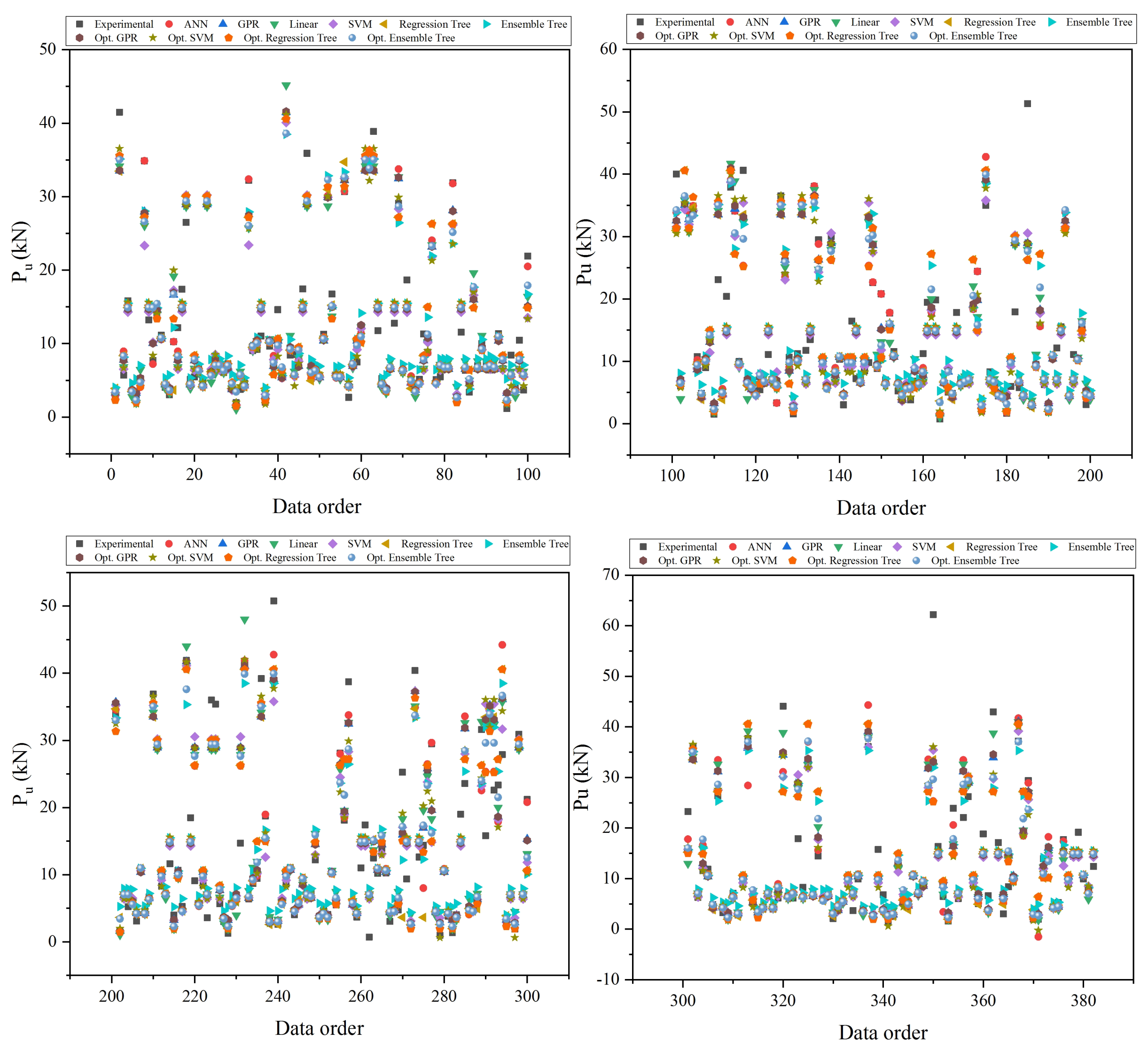
  • The error value distribution was used to assess the optimized GPR, GPR and ANN models’ resilience and accuracy. The suggested model surpasses other ML models by having the lowest absolute error values, which are confined to less than 7 to 8 kN of the P u range.
The performance of the proposed model can be further enhanced using a large number of datasets. The developed models are only valid for bond strengths ranging from 0.7 to 62.20 kN, which can be utilized for the accurate prediction of FRCM–concrete bond strength.

Author Contributions

A.K. (Aman Kumar) and O.T.: conceptualization, investigation, methodology, resources, software, writing—original draft; H.C.A., A.K. (Achara Khamaksorn) and A.M.: investigation, validation, review and editing; K.K.: conceptualization, software, writing—review and editing; M.A.M. and O.T.: writing—review and editing. All authors have read and agreed to the published version of the manuscript.

Funding

Not applicable.

Institutional Review Board Statement

Not applicable.

Informed Consent Statement

Not applicable.

Data Availability Statement

The data cannot be shared at this time due to being part of future studies.

Acknowledgments

The authors are thankful to the Director, CSIR—Central Building Research Institute, Roorkee, India, for allowing the manuscript to be published, and the authors would like to thank research network from CMU, UA and ICL for their collaboration.

Conflicts of Interest

The authors declare no conflict of interest.

References

  1. Sidiropoulos, S.; Han, K.; Majumdar, A.; Washington, Y.O. Robust identification of air traffic flow patterns in Metroplex terminal areas under demand uncertainty. Transp. Res. Part Emerg. Technol. 2017, 75, 212–227. [Google Scholar] [CrossRef]
  2. Mullard, J.A.; Stewart, M.G. Life-Cycle Cost Assessment of Maintenance Strategies for RC Structures in Chloride Environments. J. Bridge Eng. 2012, 17, 353–362. [Google Scholar] [CrossRef]
  3. Navarro, I.J.; Yepes, V.; Martí, J.V. Life Cycle Cost Assessment of Preventive Strategies Applied to Prestressed Concrete Bridges Exposed to Chlorides. Sustainability 2018, 10, 845. [Google Scholar] [CrossRef] [Green Version]
  4. Ali, B.S.; Ochieng, W.; Majumdar, A.; Schuster, W.; Chiew, T.K. ADS-B System Failure Modes and Models. J. Navig. 2014, 67, 995–1017. [Google Scholar]
  5. Firmo, J.P.; Correia, J.R.; Bisby, L.A. Bisby. Fire Behaviour of FRP-Strengthened Reinforced Concrete Structural Elements: A State-of-the-Art Review. Compos. Part B Eng. 2015, 80, 198–216. [Google Scholar] [CrossRef]
  6. Spadea, G.; Bencardino, F.; Sorrenti, F.; Swamy, R.N. Structural Effectiveness of FRP Materials in Strengthening RC Beams. Eng. Struct. 2015, 99, 631–641. [Google Scholar] [CrossRef]
  7. Tang, Y.; Yao, Y.; Cang, J. Structural and Sensing Performance of Rc Beams Strengthened with Prestressed near-Surface Mounted Self-Sensing Basalt FRP Bar. Compos. Struct. 2021, 259, 113474. [Google Scholar] [CrossRef]
  8. Saini, A.; Prakash, S.S. Analytical Study on the Effectiveness of Hybrid FRP Strengthening on Behaviour of Slender Reinforced Concrete Square Columns. Structures 2021, 33, 4218–4242. [Google Scholar] [CrossRef]
  9. Jincheng, Y.; Haghani, R.; Blanksvärd, T.; Lundgren, K. Experimental Study of Frp-Strengthened Concrete Beams with Corroded Reinforcement. Constr. Build. Mater. 2021, 301, 124076. [Google Scholar]
  10. Feng, Z.; Gao, L.; Wu, Y.-F.; Liu, J. Flexural Design of Reinforced Concrete Structures Strengthened with Hybrid Bonded FRP. Compos. Struct. 2021, 269, 113996. [Google Scholar]
  11. Ababneh, A.N.; Al-Rousan, R.Z.; Ghaith, I.M. Experimental Study on Anchoring of Frp-Strengthened Concrete Beams. Structures 2020, 23, 26–33. [Google Scholar] [CrossRef]
  12. Justas, S.; Valivonis, J. Concrete Cracking and Deflection Analysis of RC Beams Strengthened with Prestressed FRP Reinforcements under External Load Action. Compos. Struct. 2021, 225, 113036. [Google Scholar]
  13. Liangliang, W.; Ueda, T.; Matsumoto, K.; Zhu, J.-H. Experimental and Analytical Study on the Behavior of RC Beams with Externally Bonded Carbon-FRCM Composites. Compos. Struct. 2021, 273, 114291. [Google Scholar]
  14. Ahmed, M.; Refai, A.E. Assessment and Modeling of the Debonding Failure of Fabric-Reinforced Cementitious Matrix (FRCM) Systems. Compos. Struct. 2021, 275, 114394. [Google Scholar]
  15. Muhammad, K.; Abed, F. Finite Element Parametric Analysis of RC Columns Strengthened with FRCM. Compos. Struct. 2021, 275, 114498. [Google Scholar]
  16. Alemdar, B.; Hökelekli, E. A Cost-Effective FRCM Technique for Seismic Strengthening of Minarets. Eng. Struct. 2021, 229, 111672. [Google Scholar]
  17. Gaochuang, C.; Tsavdaridis, K.D.; Larbi, A.S.; Purnell, P. A Simplified Design Approach for Predicting the Flexural Behavior of TRM-Strengthened RC Beams under Cyclic Loads. Constr. Build. Mater. 2021, 285, 122799. [Google Scholar]
  18. Zhifang, D.; Deng, M.; Zhang, C.; Zhang, Y.; Sun, H. Tensile Behavior of Glass Textile Reinforced Mortar (TRM) Added with Short PVA Fibers. Constr. Build. Mater. 2021, 260, 119897. [Google Scholar]
  19. Xuan, W.; Lam, C.C.; Iu, V.P. Comparison of Different Types of TRM Composites for Strengthening Masonry Panels. Constr. Build. Mater. 2019, 219, 184–194. [Google Scholar]
  20. Shichang, L.; Yin, S. Research on the Mechanical Properties of Assembled TRC Permanent Formwork Composite Columns. Eng. Struct. 2021, 247, 113105. [Google Scholar]
  21. Ngoc, T.C.T.; Nguyen, X.H.; Nguyen, H.C.; Le, D.D. Shear Performance of Short-Span FRP-Reinforced Concrete Beams Strengthened with CFRP and TRC. Eng. Struct. 2021, 242, 112548. [Google Scholar]
  22. Tala, T.; Vu, X.H.; Michel, M.; Ferrier, E.; Larbi, A.S. Physical, Chemical and Thermomechanical Characterisation of Glass Textile-Reinforced Concretes (TRCC): Effect of Elevated Temperature and of Cementitious Matrix Nature on Properties of TRC. Mater. Today Commun. 2020, 25, 101580. [Google Scholar]
  23. Shen, L.H.; Wang, J.Y.; Xu, S.L.; Zhao, X.; Peng, Y. Physical, Flexural Behavior of Trc Contained Chopped Fibers Subjected to High Temperature. Constr. Build. Mater. 2020, 262, 120562. [Google Scholar] [CrossRef]
  24. Naser, M.Z.; Hawileh, R.A.; Abdalla, J.A. Fiber-Reinforced Polymer Composites in Strengthening Reinforced Concrete Structures: A Critical Review. Eng. Struct. 2020, 198, 109542. [Google Scholar] [CrossRef]
  25. Milani, E.G.; Ghiassi, B. Chapter 20—Advanced Finite Element Modeling of Textile-Reinforced Mortar Strengthened Masonry. In Numerical Modeling of Masonry and Historical Structures; Ghiassi, B., Milani, G., Eds.; Woodhead Publishing: Amsterdam, The Netherlands, 2019; pp. 713–743. [Google Scholar]
  26. Koutas, L.N.; Tetta, Z.; Bournas, D.A.; Triantafillou, T.C. Strengthening of Concrete Structures with Textile Reinforced Mortars: State-of-the-Art Review. J. Compos. Constr. 2019, 23, 03118001. [Google Scholar] [CrossRef]
  27. Xuan, W.; Lam, C.C.; Iu, V.P. Bond Behaviour of Steel-TRM Composites for Strengthening Masonry Elements: Experimental Testing and Numerical Modelling. Constr. Build. Mater. 2019, 253, 119157. [Google Scholar]
  28. Alexandru, C.; Kumar, A.; Vlach, T.; Laiblová, L.; Škapin, A.S.; Hájek, P. Property Improvements of Alkali Resistant Glass Fibres/Epoxy Composite with Nanosilica for Textile Reinforced Concrete Applications. Mater. Des. 2016, 89, 146–155. [Google Scholar]
  29. Scheffler, C.; Gao, S.L.; Plonka, R.; Mäder, E.; Hempel, S.; Butler, M.; Mechtcherine, V. Interphase Modification of Alkali-Resistant Glass Fibres and Carbon Fibres for Textile Reinforced Concrete I: Fibre Properties and Durability. Compos. Sci. Technol. 2009, 69, 531–538. [Google Scholar] [CrossRef]
  30. Massimo, M.; Nobili, A.; Signorini, C.; Sola, A. Effect of High Temperature Exposure on Epoxy-Coated Glass Textile Reinforced Mortar (GTRM) Composites. Constr. Build. Mater. 2019, 212, 765–774. [Google Scholar]
  31. Ayman, S.; Elgabbas, F.; Elshafie, H. Tensile Behavior of Basalt Textile-Reinforced Mortar (BTRM). Ain Shams Eng. J. 2021, 13, 101488. [Google Scholar]
  32. Xuan, C.; Zhuge, Y.; Al-Gemeel, A.N.; Xiong, Z. Compressive Behaviour of Concrete Column Confined with Basalt Textile Reinforced ECC. Eng. Struct. 2021, 243, 112651. [Google Scholar]
  33. Sai, L.; Wang, X.; Rawat, P.; Chen, Z.; Shi, C.; Zhu, D. Experimental Study and Analytical Modeling on Tensile Performance of Basalt Textile Reinforced Concrete. Constr. Build. Mater. 2021, 267, 120972. [Google Scholar]
  34. Qingxuan, W.; Ding, Y.; Randl, N. Investigation on the Alkali Resistance of Basalt Fiber and Its Textile in Different Alkaline Environments. Constr. Build. Mater. 2021, 272, 121670. [Google Scholar]
  35. Halvaei, M.; Jamshidi, M.; Latifi, M.; Ejtemaei, M. Experimental Investigation and Modelling of Flexural Properties of Carbon Textile Reinforced Concrete. Constr. Build. Mater. 2020, 262, 120877. [Google Scholar] [CrossRef]
  36. Tien, T.M.; Vu, X.H.; Ferrier, E. Experimental and Numerical Investigation of Carbon Textile/Cementitious Matrix Interfacebehaviourfrom Pull-out Tests. Constr. Build. Mater. 2021, 282, 122634. [Google Scholar]
  37. Ting, G.; Ahmed, A.H.; Curosu, I.; Mechtcherine, V. Tensile Behavior of Hybrid Fiber Reinforced Composites Made of Strain-Hardening Cement-Based Composites (SHCC) and Carbon Textile. Constr. Build. Mater. 2020, 262, 120913. [Google Scholar]
  38. Du, Y.X.; Shao, X.; Chu, S.H.; Zhou, F.; Su, R.K.L. Strengthening of Preloaded RC Beams Using Prestressed Carbon Textile Reinforced Mortar Plates. Structures 2021, 30, 735–744. [Google Scholar] [CrossRef]
  39. Goliath, K.B.; Cardoso, D.C.; Silva, F.D. Flexural Behavior of Carbon-Textile-Reinforced Concrete I-Section Beams. Compos. Struct. 2021, 260, 113540. [Google Scholar] [CrossRef]
  40. Aljazaeri Zena, R.; John, J.M. Fatigue and Flexural Behavior of Reinforced-Concrete Beams Strengthened with Fiber-Reinforced Cementitious Matrix. J. Compos. Constr. 2017, 21, 04016075. [Google Scholar] [CrossRef]
  41. Pino, V.; Akbari Hadad, H.; De Caso y Basalo, F.; Nanni, A. Performance of Frcm-Strengthened Rc Beams Subject to Fatigue. J. Bridge Eng. 2017, 22, 04017079. [Google Scholar] [CrossRef]
  42. Emre, A.; Rashidi, M. Axial Behavior of Concrete Confined with Flax Fiber-Reinforced Polymers. Mater. Today Commun. 2021, 28, 102646. [Google Scholar]
  43. Giuseppe, F.; Pepe, M.; Martinelli, E.; Filho, R.D.T. Tensile Behavior of Flax Textile Reinforced Lime-Mortar: Influence of Reinforcement Amount and Textile Impregnation. Cem. Concr. Compos. 2021, 119, 103984. [Google Scholar]
  44. Farinha, C.B.; de Brito, J.; Veiga, R. Incorporation of High Contents of Textile, Acrylic and Glass Waste Fibres in Cement-Based Mortars. Influence on Mortars’ Fresh, Mechanical and Deformability Behaviour. Constr. Build. Mater. 2021, 303, 124424. [Google Scholar] [CrossRef]
  45. Bello, D.C.; Brito, C.; Boem, I.; Cecchi, A.; Gattesco, N.; Oliveira, D.V. Experimental Tests for the Characterization of Sisal Fiber Reinforced Cementitious Matrix for Strengthening Masonry Structures. Constr. Build. Mater. 2019, 219, 44–55. [Google Scholar] [CrossRef] [Green Version]
  46. Rambo, D.A.S.; de Oliveira, C.U.; Salvador, R.P.; Toledo Filho, R.D.; Gomes, O.D.F.M.; de Andrade Silva, F.; de Melo Vieira, M. Sisal Textile Reinforced Concrete: Improving Tensile Strength and Bonding through Peeling and Nano-Silica Treatment. Constr. Build. Mater. 2021, 301, 124300. [Google Scholar] [CrossRef]
  47. De Souza Castoldi, R.; de Souza, L.M.S.; de Andrade Silva, F. Comparative Study on the Mechanical Behavior and Durability of Polypropylene and Sisal Fiber Reinforced Concretes. Constr. Build. Mater. 2019, 211, 617–628. [Google Scholar] [CrossRef]
  48. Jung, K.; Hong, K.; Han, S.; Park, J.; Kim, J. Prediction of Flexural Capacity of RC Beams Strengthened in Flexure with FRP Fabric and Cementitious Matrix. Int. J. Polym. Sci. 2015, 2015, 868541. [Google Scholar] [CrossRef] [Green Version]
  49. Chen, S.-Z.; Zhang, S.-Y.; Han, W.-S.; Wu, G. Ensemble learning based approach for FRP-concrete bond strength prediction. Constr. Build. Mater. 2021, 302, 124230. [Google Scholar] [CrossRef]
  50. Basran, B.; Kalkan, I.; Bergil, E.; Erdal, E. Estimation of the FRP-concrete bond strength with code formulations and machine learning algorithms. Compos. Struct. 2021, 268, 113972. [Google Scholar] [CrossRef]
  51. Aghabalaei Baghaei, K.; Hadigheh, S.A. Durability assessment of FRP-to-concrete bonded connections under moisture condition using data-driven machine learning-based approaches. Compos. Struct. 2021, 114576. [Google Scholar] [CrossRef]
  52. Su, M.; Zhong, Q.; Peng, H.; Li, S. Selected machine learning approaches for predicting the interfacial bond strength between FRPs and concrete. Constr. Build. Mater. 2021, 270, 121456. [Google Scholar] [CrossRef]
  53. Wang, X.; Liu, Y.; Xin, H. Bond strength prediction of concrete-encased steel structures using hybrid machine learning method. Structures 2021, 32, 2279–2292. [Google Scholar] [CrossRef]
  54. Sun, J.; Wang, X.; Zhang, J.; Xiao, F.; Sun, Y.; Ren, Z.; Zhang, G.; Liu, S.; Wang, Y. Multi-objective optimisation of a graphite-slag conductive composite applying a BAS-SVR based model. J. Build. Eng. 2021, 44, 103223. [Google Scholar] [CrossRef]
  55. Abuodeh, O.R.; Abdalla, J.A.; Hawileh, R.A. Prediction of shear strength and behavior of RC beams strengthened with externally bonded FRP sheets using machine learning techniques. Compos. Struct. 2020, 234, 111698. [Google Scholar] [CrossRef]
  56. Nikoo, M.; Aminnejad, B.; Lork, A. Predicting Shear Strength in FRP-Reinforced Concrete Beams Using Bat Algorithm-Based Artificial Neural Network. Adv. Mater. Sci. Eng. 2021, 2021, 5899356. [Google Scholar] [CrossRef]
  57. Alam, M.S.; Sultana, N.; Hossain, S.M.Z. Bayesian optimization algorithm based support vector regression analysis for estimation of shear capacity of FRP reinforced concrete members. Appl. Soft Comput. 2021, 105, 107281. [Google Scholar] [CrossRef]
  58. Chou, J.-S.; Pham, T.-P.-T.; Nguyen, T.-K.; Pham, A.-D.; Ngo, N.-T. Shear strength prediction of reinforced concrete beams by baseline, ensemble, and hybrid machine learning models. Soft Comput. 2020, 24, 3393–3411. [Google Scholar] [CrossRef]
  59. Fu, B.; Feng, D.-C. A machine learning-based time-dependent shear strength model for corroded reinforced concrete beams. J. Build. Eng. 2021, 36, 102118. [Google Scholar] [CrossRef]
  60. Gao, J.; Koopialipoor, M.; Armaghani, D.J.; Ghabussi, A.; Baharom, S.; Morasaei, A.; Shariati, A.; Khorami, M.; Zhou, J. Evaluating the bond strength of FRP in concrete samples using machine learning methods. Smart Struct. Syst. 2020, 26, 403–418. [Google Scholar]
  61. Su, M.; Peng, H.; Yuan, M.; Li, S. Identification of the interfacial cohesive law parameters of FRP strips externally bonded to concrete using machine learning techniques. Eng. Fract. Mech. 2021, 247, 107643. [Google Scholar] [CrossRef]
  62. Naser, M.Z. Machine Learning Assessment of Fiber-Reinforced Polymer-Strengthened and Reinforced Concrete Members. ACI Struct. J. 2021, 117, 237–251. [Google Scholar]
  63. He, M.; Wang, Y.; Ramakrishnan, K.R.; Zhang, Z. A comparison of machine learning algorithms for assessment of delamination in fiber-reinforced polymer composite beams. Struct. Health Monit. 2020, 20, 1997–2012. [Google Scholar] [CrossRef]
  64. Almustafa, M.K.; Nehdi, M.L. Machine learning prediction of structural response for FRP retrofitted RC slabs subjected to blast loading. Eng. Struct. 2021, 244, 112752. [Google Scholar] [CrossRef]
  65. Alwanas, A.A.H.; Al-Musawi, A.A.; Salih, S.Q.; Tao, H.; Ali, M.; Yaseen, Z.M. Load-carrying capacity and mode failure simulation of beam-column joint connection: Application of self-tuning machine learning model. Eng. Struct. 2019, 194, 220–229. [Google Scholar] [CrossRef]
  66. Rezaiee-Pajand, M.; Karimipour, A.; Abad, J.M.N. Crack Spacing Prediction of Fibre-Reinforced Concrete Beams with Lap-Spliced Bars by Machine Learning Models. Iran. J. Sci. Technol. Trans. Civ. Eng. 2021, 45, 833–850. [Google Scholar] [CrossRef]
  67. Nguyen, H.D.; Zhang, Q.; Choi, E.; Duan, W. An improved deflection model for FRP RC beams using an artificial intelligence-based approach. Eng. Struct. 2020, 219, 110793. [Google Scholar] [CrossRef]
  68. Bencardino, F.; Condello, A.; Ashour, A.F. Single-lap shear bond tests on Steel Reinforced Geopolymeric Matrix-concrete joints. Compos. Part B Eng. 2017, 110, 62–71. [Google Scholar] [CrossRef] [Green Version]
  69. Caggegi, C.; Sciuto, D.; Cuomo, M. Experimental study on effective bond length of basalt textile reinforced mortar strengthening system: Contributions of digital image correlation. Measurement 2018, 129, 119–127. [Google Scholar] [CrossRef]
  70. Sneed, L.H.; D’Antino, T.; Carloni, C.; Pellegrino, C. A comparison of the bond behavior of PBO-FRCM composites determined by double-lap and single-lap shear tests. Cem. Concr. Compos. 2015, 64, 37–48. [Google Scholar] [CrossRef]
  71. De Felice, G.; Aiello, M.A.; Caggegi, C.; Ceroni, F.; De Santis, S.; Garbin, E.; Viskovic, A. Recommendation of RILEM Technical Committee 250-CSM: Test method for Textile Reinforced Mortar to substrate bond characterization. Mater. Struct. 2018, 51, 1–9. [Google Scholar] [CrossRef]
  72. Raoof, S.M.; Bournas, D.A. Bond between TRM versus FRP composites and concrete at high temperatures. Compos. Part B Eng. 2017, 127, 150–165. [Google Scholar] [CrossRef]
  73. Carloni, C.; D’Antino, T.; Sneed, L.H.; Pellegrino, C. Role of the Matrix Layers in the Stress-Transfer Mechanism of FRCM Composites Bonded to a Concrete Substrate. J. Eng. Mech. 2015, 141, 04014165. [Google Scholar] [CrossRef]
  74. Friedman, J.; Hastie, J.; Tibshirani, R. The Elements of Statistical Learning; Springer: New York, NY, USA, 2009. [Google Scholar]
  75. D’Ambrisi, A.; Feo, L.; Focacci, F. Experimental analysis on bond between PBO-FRCM strengthening materials and concrete. Compos. Part Eng. 2013, 44, 524–532. [Google Scholar] [CrossRef]
  76. Awani, O.; Refai, A.E.; El-Maaddawy, T. Bond characteristics of carbon fabric-reinforced cementitious matrix in double shear tests. Constr. Build. Mater. 2015, 101, 39–49. [Google Scholar] [CrossRef]
  77. Raoof, S.M.; Koutas, L.N.; Bournas, D.A. Bond between textile-reinforced mortar (TRM) and concrete substrates: Experimental investigation. Compos. Part B Eng. 2016, 98, 350–361. [Google Scholar] [CrossRef]
  78. Younis, A.; Ebead, U. Bond characteristics of different FRCM systems. Constr. Build. Mater. 2018, 175, 610–620. [Google Scholar] [CrossRef]
  79. Li, S.; Yin, S.; Gao, Y. Analysis of Interface Properties Between TRC and Concrete Under Chloride Attack Based on Fracture Energy. Int. J. Concr. Struct. Mater. 2020, 14, 28. [Google Scholar] [CrossRef]
  80. Tran, C.T.M.; Stitmannaithum, B.; Ueda, T. Investigation of The Bond Behaviour Between PBO-FRCM Strengthening Material and Concrete. J. Adv. Concr. Technol. 2014, 12, 545–557. [Google Scholar] [CrossRef] [Green Version]
  81. Sneed, L.H.; D’Antino, T.; Carloni, C. Investigation of Bond Behavior of PBO Fiber-Reinforced Cementitious Matrix Composite-Concrete Interface. Mater. J. 2014, 111, 569–580. [Google Scholar]
  82. Ceroni, F.; Bonati, A.; Galimberti, V.; Occhiuzzi, A. Effects of Environmental Conditioning on the Bond Behavior of FRP and FRCM Systems Applied to Concrete Elements. J. Eng. Mech. 2018, 144, 04017144. [Google Scholar] [CrossRef]
  83. D’Antino, T.; Sneed, L.H.; Carloni, C.; Pellegrino, C. Influence of the substrate characteristics on the bond behavior of PBO FRCM-concrete joints. Constr. Build. Mater. 2015, 101, 838–850. [Google Scholar] [CrossRef]
  84. Chaabene, W.B.; Flah, M.; Nehdi, M.L. Machine learning prediction of mechanical properties of concrete: Critical review. Constr. Build. Mater. 2020, 260, 119889. [Google Scholar] [CrossRef]
  85. Tripepi, G.; Jager, K.J.; Dekker, F.W.; Zoccali, C. Linear and logistic regression analysis. Kidney Int. 2008, 73, 806–810. [Google Scholar] [CrossRef] [PubMed] [Green Version]
  86. Montgomery Douglas, C.; Peck, E.A.; Vining, G.G. Linear and logistic regression analysis. In Introduction to Linear Regression Analysis; John Wiley and Sons: Hoboken, NJ, USA, 2021. [Google Scholar]
  87. Loh, W.Y. Classification and regression trees. Wiley Interdiscip. Rev. Data Min. Knowl. Discov. 2011, 1, 14–23. [Google Scholar] [CrossRef]
  88. Mur, R.; Díaz, I.; Rodríguez, M. Comparative Study of Surrogate Modelling Techniques Applied to Three Different Chemical Processes. Comput. Aided Chem. Eng. 2020, 48, 145–150. [Google Scholar]
  89. Richardson, R.R.; Osborne, M.A.; Howey, D.A. Gaussian process regression for forecasting battery state of health. J. Power Sources 2017, 357, 209–219. [Google Scholar] [CrossRef]
  90. Cheng, L.; Ramchandran, S.; Vatanen, T.; Lietzén, N.; Lahesmaa, R.; Vehtari, A.; Lähdesmäki, H. An additive Gaussian process regression model for interpretable non-parametric analysis of longitudinal data. Nat. Commun. 2019, 10, 1798. [Google Scholar] [CrossRef] [PubMed]
  91. Lubbe, F.; Maritz, J.; Harms, T. Evaluating the Potential of Gaussian Process Regression for Solar Radiation Forecasting: A Case Study. Energies 2020, 13, 5509. [Google Scholar] [CrossRef]
  92. Asante-Okyere, S.; Shen, C.; Yevenyo Ziggah, Y.; Moses Rulegeya, M.; Zhu, X. Investigating the Predictive Performance of Gaussian Process Regression in Evaluating Reservoir Porosity and Permeability. Energies 2018, 11, 3261. [Google Scholar] [CrossRef] [Green Version]
  93. Zimmermann, A. TEnsemble-Trees: Leveraging Ensemble Power Inside Decision Trees. In Proceedings of the International Conference on Discovery Science, Budapest, Hungary, 13–16 October 2008; Springer: Heidelberg, Germany, 2008. [Google Scholar]
  94. Jerome, H.F. Greedy function approximation: A gradient boosting machine. Ann. Stat. 2001, 29, 1189–1232. [Google Scholar]
  95. Peterson, K.D. Resting heart rate variability can predict track and field sprint performance. OA J. Sports 2018, 1, 1–9. [Google Scholar]
  96. McCulloch, W.S.; Pitts, W. A logical calculus of the ideas immanent in nervous activity. Bull. Math. Biophys. 1943, 5, 115–133. [Google Scholar] [CrossRef]
  97. Firat, M.; Turan, M.E.; Yurdusev, M.A. Comparative analysis of neural network techniques for predicting water consumption time series. J. Hydrol. 2010, 384, 46–51. [Google Scholar] [CrossRef]
  98. Abbasi, M.; El Hanandeh, A. Forecasting municipal solid waste generation using artificial intelligence modelling approaches. Waste Manag. 2016, 56, 13–22. [Google Scholar] [CrossRef] [PubMed]
  99. Mashrei, M.A.; Seracino, R.; Rahman, M.S. Application of artificial neural networks to predict the bond strength of FRP-to-concrete joints. Constr. Build. Mater. 2013, 40, 812–821. [Google Scholar] [CrossRef]
  100. Jahangir, H.; Rezazadeh Eidgahee, D. A new and robust hybrid artificial bee colony algorithm—ANN model for FRP-concrete bond strength evaluation. Compos. Struct. 2021, 257, 113160. [Google Scholar] [CrossRef]
Figure 1. Types of FRCM.
Sustainability 14 00845 g001
Figure 2. RILEM guidelines for bond characterization.
Sustainability 14 00845 g002
Figure 3. Configurations shear test: (a) Single-lap shear test; (b) double-lap shear test.
Sustainability 14 00845 g003
Figure 4. Methodology of present work.
Sustainability 14 00845 g004
Figure 5. Relative frequency distribution of experimental datasets.
Sustainability 14 00845 g005
Figure 6. Plotmatrix of normalized dataset.
Sustainability 14 00845 g006
Figure 7. Boosted regression tree [95].
Sustainability 14 00845 g007
Figure 8. Bagging regression tree [95].
Sustainability 14 00845 g008
Figure 9. Neural network architecture.
Sustainability 14 00845 g009
Figure 10. Comparison of machine learning models.
Sustainability 14 00845 g010
Figure 11. R, RMSE, MAPE and MAE compression of best prediction models.
Sustainability 14 00845 g011
Figure 12. Comparison of ML predicted results with experimental results with respect to data order.
Sustainability 14 00845 g012
Figure 13. Experimental and predicted bond strength calculated by ANN, ensemble tree, GPR, linear regression, regression tree and SVM.
Sustainability 14 00845 g013
Figure 14. Experimental and predicted bond strength calculated by optimized GPR, optimized regression tree, optimized SVM and optimized ensemble tree.
Sustainability 14 00845 g014
Figure 15. Absolute error values of prediction models.
Sustainability 14 00845 g015
Table 1. Extracted data of FRCM–concrete bond.
Referencenb c (mm)f c k (MPa)t f (mm)b f (mm)L f (mm)f f (MPa)E f (GPa)P u (KN)
 [75]1100301010050–2505213–5391271–2735.19–15.64
[76]1150555–1075–15075–15038002308.34–44.1
[77]1–410014.7–32.868050–45038002257.7–50.75
[72]3–410029.7–33.76802001518166.89.1–62.2
[68]115016.8850100–400147073.54.76–7.9
[69]112020.6109050–2601089561.984–5.746
[70]112533.51034–100100–45030142063–21.21
[78]1–21003010–1310075–200767–123580–2703.34–29.5
[79]110040–59.36–860–100100–3304660–4700231–2400.78–3.97
[80]110039–4112100250–40058002788.98–11.86
[81]1–212542.54–834–60100–33058002700.97–8.29
[82]115050105015044002607.24–20.39
[83]112526.9–33.51060–80330–45030142060.7–10.01
Table 2. Statistical features of the gathered database.
ParameterSymbol UsedUnitTypeMeanMin.Max.Std.
FRCMn-Input1.5105140.8925
t f mmInput8.70944132.2028
b f mmInput72.66493415024.0303
L f mmInput232.866550450109.7950
f f MPaInput3584.0376758001574.20
E f GPaInput213.49325627862.0064
Concreteb c mmInput120.458110015017.6764
f c k MPaInput35.993714.700059.309.8866
P u -kNOutput12.74730.700062.200011.2335
Table 3. Comparison of performance indices of different models.
ModelData TypeRRMSEMAPE (%)MAE
ANNTraining0.95383.295218.31711.5887
Testing0.88715.452522.86262.8800
Overall0.93214.023824.10892.2290
GPRTraining0.94353.644224.21882.0179
Testing0.91304.790323.85392.7193
Overall0.93364.023824.10892.2291
SVMTraining0.93293.965724.42482.1105
Testing0.90515.034824.80172.7395
Overall0.92394.315524.53832.2998
LinearTraining0.93603.862325.70762.2904
Testing0.91274.805628.48082.8437
Overall0.92844.168826.54252.4570
Regression TreeTraining0.92874.070526.23882.3611
Testing0.87295.782826.01523.2303
Overall0.91024.652726.17152.6228
EnsembleTraining0.93014.170141.16322.7784
Testing0.89295.372040.25153.2918
Overall0.91764.565440.88872.9330
Optimized GPRTraining0.94323.652624.34012.0286
Testing0.91374.773123.73432.7112
Overall0.93364.022924.15772.2341
Optimized SVMTraining0.93533.894419.93811.9364
Testing0.91134.873020.76242.6893
Overall0.92754.213020.18632.1631
Optimized EnsembleTraining0.94043.747524.46642.1357
Testing0.90425.044322.70602.7824
Overall0.92864.180423.93642.3303
Optimized Regression TreeTraining0.93293.952422.6536.2475
Testing0.88225.550722.50352.9251
Overall0.91634.494422.73462.4553
Publisher’s Note: MDPI stays neutral with regard to jurisdictional claims in published maps and institutional affiliations.

