Towards Incompressible Laminar Flow Estimation Based on Interpolated Feature Generation and Deep Learning

Abstract

For industrial design and the improvement of fluid flow simulations, computational fluid dynamics (CFD) solvers offer practical functions and conveniences. However, because iterative simulations demand lengthy computation times and a considerable amount of memory for sophisticated calculations, CFD solvers are not economically viable. Such limitations are overcome by CFD data-driven learning models based on neural networks, which lower the trade-off between accurate simulation performance and model complexity. Deep neural networks (DNNs) or convolutional neural networks (CNNs) are good illustrations of deep learning-based CFD models for fluid flow modeling. However, improving the accuracy of fluid flow reconstruction or estimation in these earlier methods is crucial. Based on interpolated feature data generation and a deep U-Net learning model, this work suggests a rapid laminar flow prediction model for inference of Naiver–Stokes solutions. The simulated dataset consists of 2D obstacles in various positions and orientations, including cylinders, triangles, rectangles, and pentagons. The accuracy of estimating velocities and pressure fields with minimal relative errors can be improved using this cutting-edge technique in training and testing procedures. Tasks involving CFD design and optimization should benefit from the experimental findings.

1. Introduction

Computational fluid dynamics (CFD) simulations are employed in several fields, such as mechanical engineering, medicine, and civil engineering. CFD solvers are numerical tools for simulating fluid flow characteristics to design, analyze, or optimize fluid flow behavior. However, high temporal and spatial resolution is required to achieve high accuracy in state-of-the-art CFD simulations. These solvers require expensive computational resources, especially with iterative problems. To this end, data-driven machine learning models not only estimate accurate approximation fluid flow fields, but also require fewer computational resources [1]. To reduce computational costs, a trained neural network (NN) might take the role of a portion of the numerical resolution process. As an illustration, several NN applications have been produced to solve and predict flow in terms of the large eddy simulation (LES) [2] and Reynolds-averaged Navier–Stokes (RANS) computations [3,4].

CFD simulations’ complexity might be reduced by using reduced order model (ROM) techniques, such as simplified physics methods, reduced basis (RB), or proper orthogonal decomposition (POD). In particular, deep learning (DL)-enabled ROM can be used to set up a nonlinear relationship between various inputs and outputs of a target system. The DL-enabled ROM, along with the training model, can generate a low-dimensional subspace that records the average behavior of flows. Through this training process, complex features that cannot be expressed explicitly in a functional form can be represented [5]. In practice, the DL-enabled ROM accurately captures fluid flow’s temporal and spatial nonlinear features. For example, Wang et al. [6] presented a model recognition of reduced-order fluid dynamic systems by DL. The authors proved that their framework could capture complex fluid dynamics features with less computational cost. Furthermore, Fukami et al. [7] performed a super-resolution analysis of evidently under-resolved turbulent flow data based on the DL model and then reconstructed the high-resolution flow field. This successful model built a nonlinear mapping between low and high resolutions of the turbulent flow fields.

The various proposed DL-ROM algorithms [8,9] were evaluated on both linear and nonlinear time-dependent parameters to demonstrate the flexibility of this methodology and its incredible computing savings. After executing a prior dimensional reduction by POD, Fresca et al. [10] suggested that DL-based ROMs rely on DNNs, significantly reducing their training times. The blood flow in a cerebral aneurysm, the fluid-structure interaction between an elastic beam attached to a fixed, rigid block, and the flow around a cylindrical benchmark are all accurately predicted by the resulting POD-DL-ROMs in almost real-time. A novel DL framework called DL-ROM was also developed by Pant et al. [11] to build a neural network that can make non-linear projections to lower-order states. They then employ a 3D autoencoder and 3D U-Net-based architectures to effectively forecast future time steps of the simulation using the learned reduced state. By traversing time in the learned reduced state, their model DL-ROM can efficiently anticipate future time steps by building highly accurate reconstructions from the learned ROM. Recently, Kang et al. [12] presented POD-ROM, which quickly and precisely describes the flow status of the fluid field in rod bundles.

DL-based CFD models have recently attracted the attention of fluid flow and thermal engineering research as a reduced-order modeling method. To learn the solutions of parametric partial differential equations (PDEs) over irregular domains, including Navier–Stokes and heat transfer equations, Gao et al. [13] presented a physics-constrained convolutional neural network (CNN) architecture. Their findings showed how well the DL technique predicted temperature and velocity fields. The DL-based CFD model was employed by San et al. [14] to precisely resolve the spatial–temporal nonlinear characteristic in a fluid dynamic system. In addition, a data-driven DL model was also used by Sekar et al. [15] to measure laminar flow on an airfoil dataset. The experimental findings demonstrated that the model accurately predicted laminar flow fields using the airfoil geometry, Reynolds number, and attack angles as learning parameters. Jin et al. [16] subsequently suggested a CFD approach based on DL that directly maps the relationship between the pressure and velocity distribution on the surface of a cylinder to determine the fluctuating velocity field around it. The aforementioned studies proved and validated the capacity of DL-based CFD to offer substitute numerical solutions to physical issues.

Guo et al. [17] and Ribeiro et al. [18] are representative pioneers of DL-based CFD model approaches. The authors used CNN and U-Net models to evaluate the proposed methods to predict steady flow around obstacles and different loss types. In this study, we present a novel approach to effectively enhance the CFD fluid flow field prediction results, using the basic concept of a DL-enabled ROM in these pioneering studies. Similar to other data-driven DL-based CFD methods, we performed design and CFD simulations using an appropriate CFD solution in advance in the offline phase. Subsequently, we obtained a raw CFD dataset and preprocessed the data to feed into the DL model. Then, the trained CFD model was used to test and evaluate the unseen CFD data case. The proposed CFD learning model results are significantly faster than a CFD simulation. The three main contributions of this paper are summarized as follows.

• Firstly, we create the raw laminar flow datasets around different obstacles using the CFD solver FEATool [19]. Then, we generate novel learning input and output interpolated CFD features using the mesh-grid and grid-data computations on these raw simulated datasets.
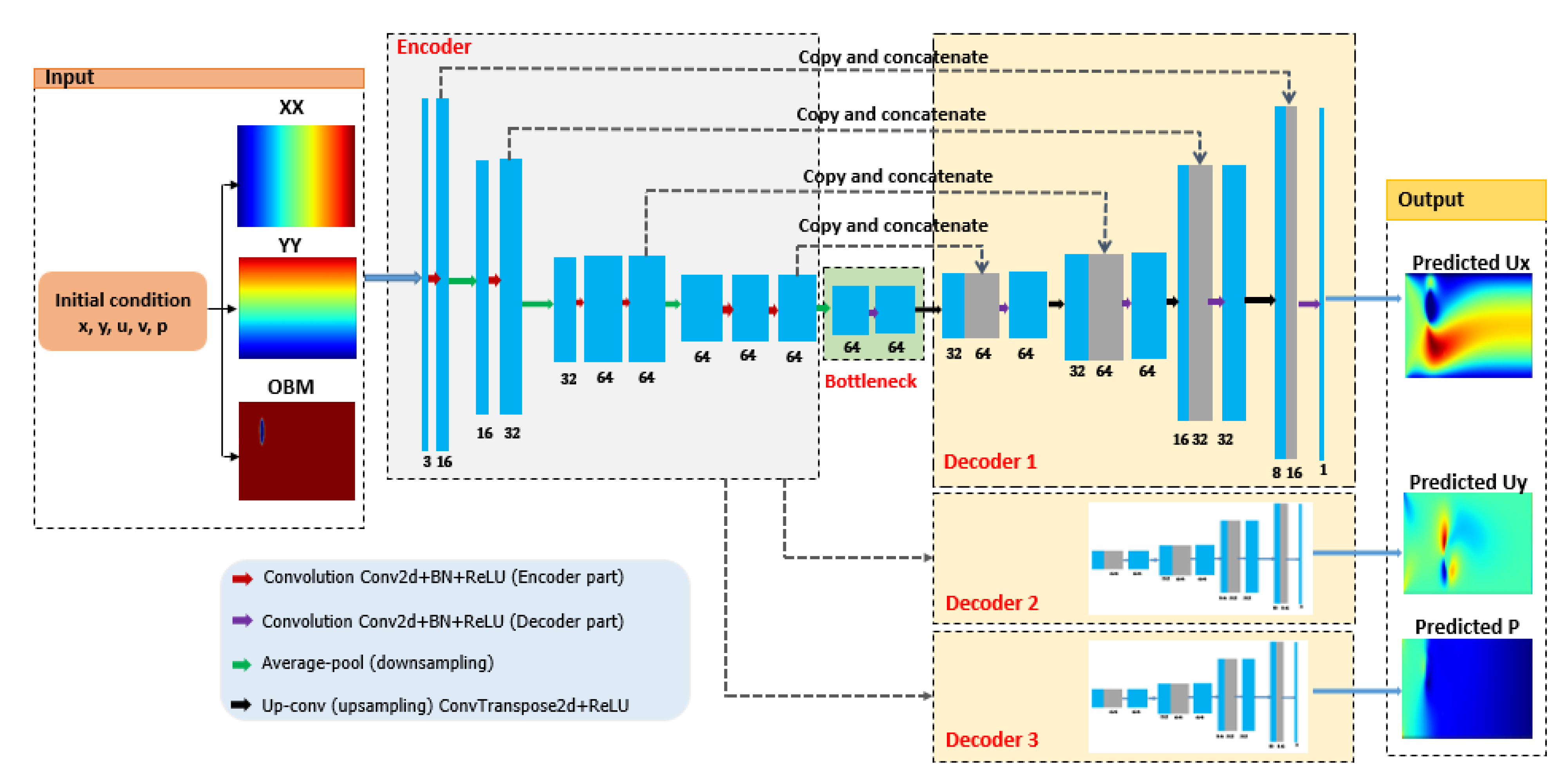
• Second, we build a deep U-Net model comprising an encoder and three decoders to predict three output classes corresponding to three different flow fields, respectively. This deep U-Net model estimates fluid flow fields by learning from preprocessed data, that is, interpolated features data.
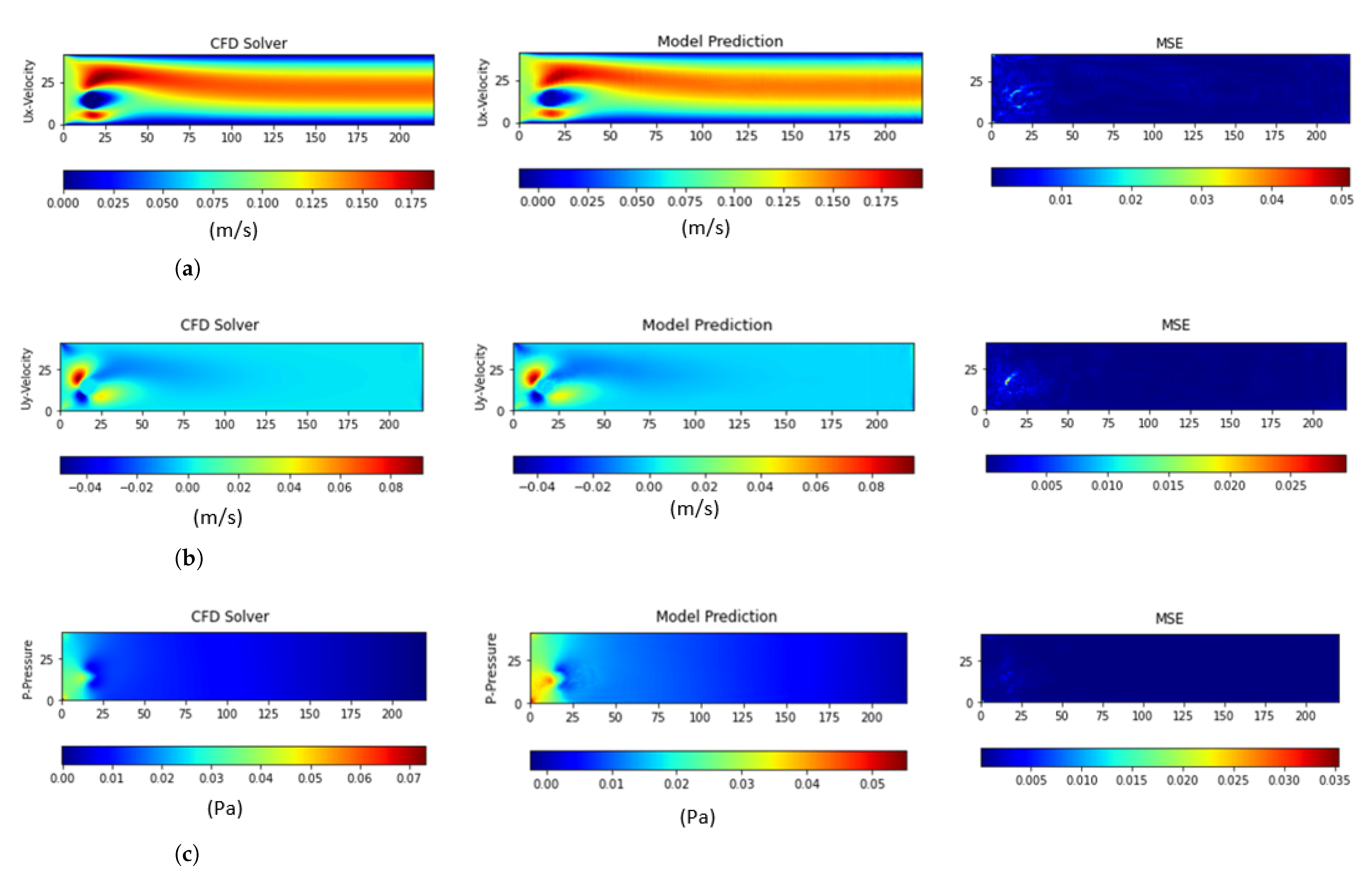
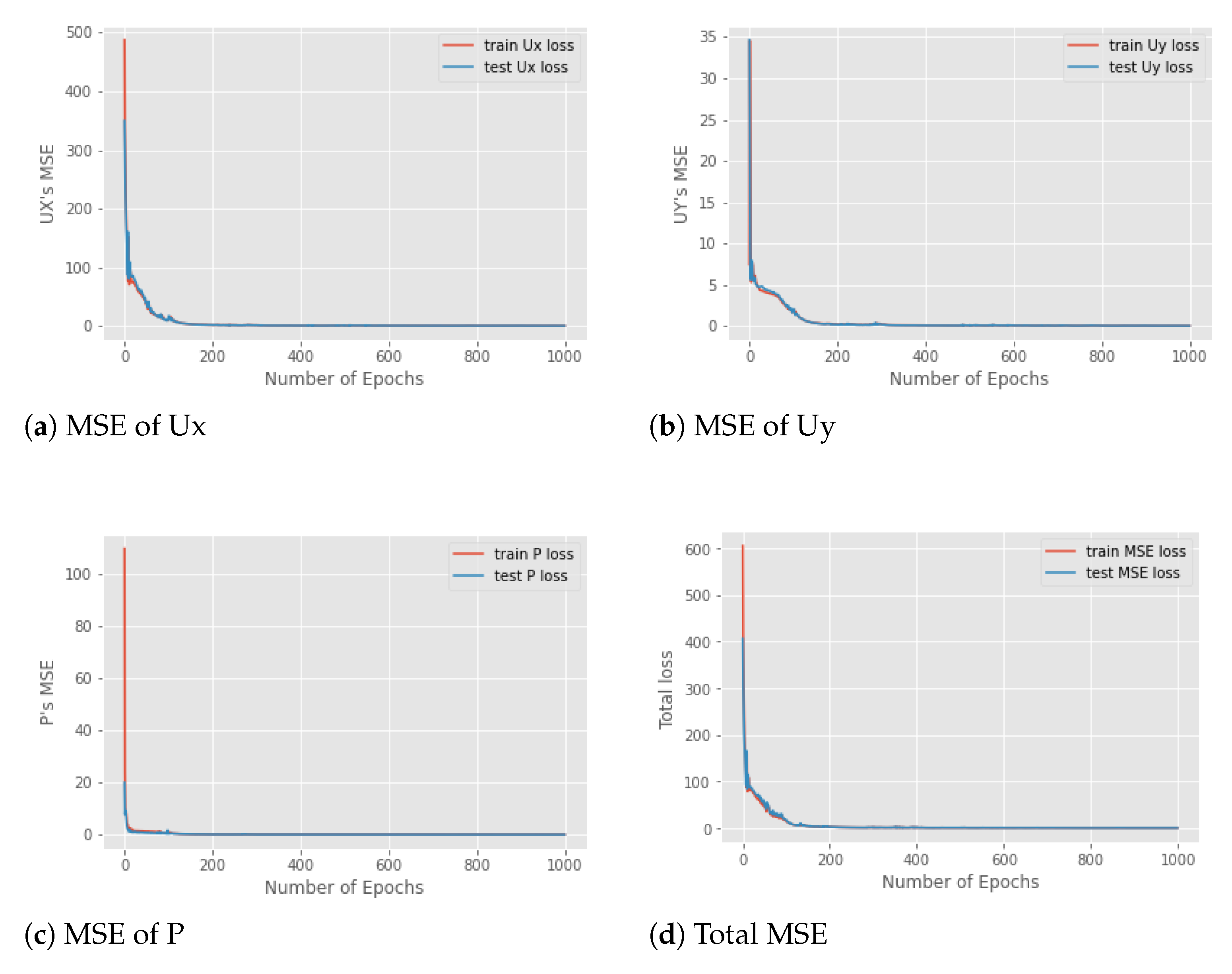
• Lastly, we evaluate the proposed method by measuring the learning and testing loss metrics. The experimental results show the competition and promise of the proposed method with other baseline models on the same dataset.

The remainder of this paper is organized as follows. The related works are described in Section 2. Section 3 presents the proposed method, including the novel learning feature data generation, DL model approach, model evaluation, and optimization. Section 4 presents the experimental results, discusses the hyper-parameters’ effectiveness, and presents a comparison with other related baseline models. Finally, Section 5 concludes the paper and discusses the scope for future work.

2. Related Work

Recent advances in ML have impacted CFD research owing to its significant advantages. ML models estimate approximate thermal or fluid flow fields with low cost and accuracy compared with conventional CFD simulations. Sarghini et al. [20] developed ML model to estimate steady-state velocity flows. Next, Lee et al. [21] built an NN to predict unsteady flow around a cylinder. The authors minimized the physical loss function comprising conservation laws and regression errors. Kashefi et al. [22] created an artificial neural network with modest geometry alterations to achieve various velocity and pressure fields. Furthermore, additional recent publications have demonstrated a variety of effective uses for CFD-based DL models, including physics-informed NN [3], airfoil design optimization [23], and acceleration of sparse linear system solutions [24,25].

The modern DL technique has recently played a vital role in CFD simulations. Deep neural network models have been used as data-driven surrogate models that efficiently approximate the velocity and pressure fields. Regarding the DL-based CFD approach, the direct estimation of fluid flow fields comprises two representative models: CNN-based CFD and variant autoencoder (AE)-based CFD.

In terms of a CNN-based CFD prediction approach, Guo et al. [17] proposed a CNN model for predicting stationary flow fields around solid objects. Moreover, previous studies [26,27] have used CNN models to learn arbitrary geometry representations. Georgiou et al. [28] developed a CNN application for reconstructing fluid force and flow prediction. Jin et al. [16] proposed a fusion CNN model to predict velocity snapshots around a cylinder. Furthermore, Zhang et al. [29] predicted the lift and drag coefficients of 2D airfoils using a CNN model. In addition, the CNN model was applied to measure flow in arbitrary shapes by Viquerat et al. [30].

In terms of AE and its variant U-Net model-based CFD prediction approach, AE models were used for supervised learning to predict various full-field flows in [16,17,21]. Especially among the various AE architectures, the U-Net model was recently applied successfully to estimate CFD flows. According to Ronneberger et al. [31], U-Net models might achieve the best segmentation accuracy by fusing high-level latent-space representation with low-level characteristics. Thuerey et al. [32] applied the U-Net model to estimate turbulent flow around airfoils, including the velocity and pressure flows, which were computed using RANS. Fukami at el. [7] applied the U-Net model to reconstruct turbulence with remarkable accuracy from rough flow field images. A recurrent U-Net architecture was investigated and developed by Kamrava et al. [33] to predict stationary velocity and pressure fields in porous membranes. Wang at el. [34] proposed a gated U-Net-based pixel CNN++ architecture to simulate fluids in porous media. Ribeiro et al. [18] applied the high-performance accuracy of the U-Net model to steady-state laminar flow approximation around simple obstacles. Chen et al. [35] proposed a twin-decoder based on the U-Net model to reconstruct incompressible laminar flow on 2D obstacle data.

In addition, the flow field feature information is crucial for enhancing the performance accuracy of flow estimation models. For example, Ribeiro et al. [18] and Alvaro et al. [33] reported remarkable prediction results through deep CFD models to predict the velocities and pressure by generating features based on the signed distance function (SDF) and flow region channel. Peng et al. [36] generated network input learning using the SDF and temperature field from numerical simulation data as output learning to feed the CNN model. SDF and binary features were developed for CFD input learning of CNN and U-Net models in [37]. Li et al. [38] proposed a wall distance field and space coordinate field for the U-Net model’s input features. In this study, we used a different approach to generate novel input features for our proposed model. Three-channel input features were extracted, including interpolated grid X and Y coordinates and obstacle binary map values. The proposed method for data generation is presented in detail in Section 3.

3. The Proposed Method

In this section, we describe the proposed method. The proposed method was trained on a dataset comprising CFD-computed laminar flows around cylindrical, triangular, rectangular, and polygonal obstacles with random 2D shapes. Figure 1 shows the proposed network architecture. This architecture’s three main parts are data generation, preprocessing deep U-Net-based CFD flow prediction, and model evaluation. The following subsections present the detailed components of the architecture.

3.1. Data Generation and Preprocessing

This section represents CFD data generation and preprocessing, which are used for deep learning networks, as shown in Figure 2. Personal data generation processing includes three steps as follows. The first step was generating arbitrary obstacles using MATLAB’s FEATool solver. The next step is to solve the Naiver–Stokes equations using the immersed method. The final step is to obtain CFD fluid fields comprising coordinates (x, y), velocities (u, v), and pressure (p). Triangular meshes were used to project the velocities and pressure fields for preprocessing and training on deep learning networks.

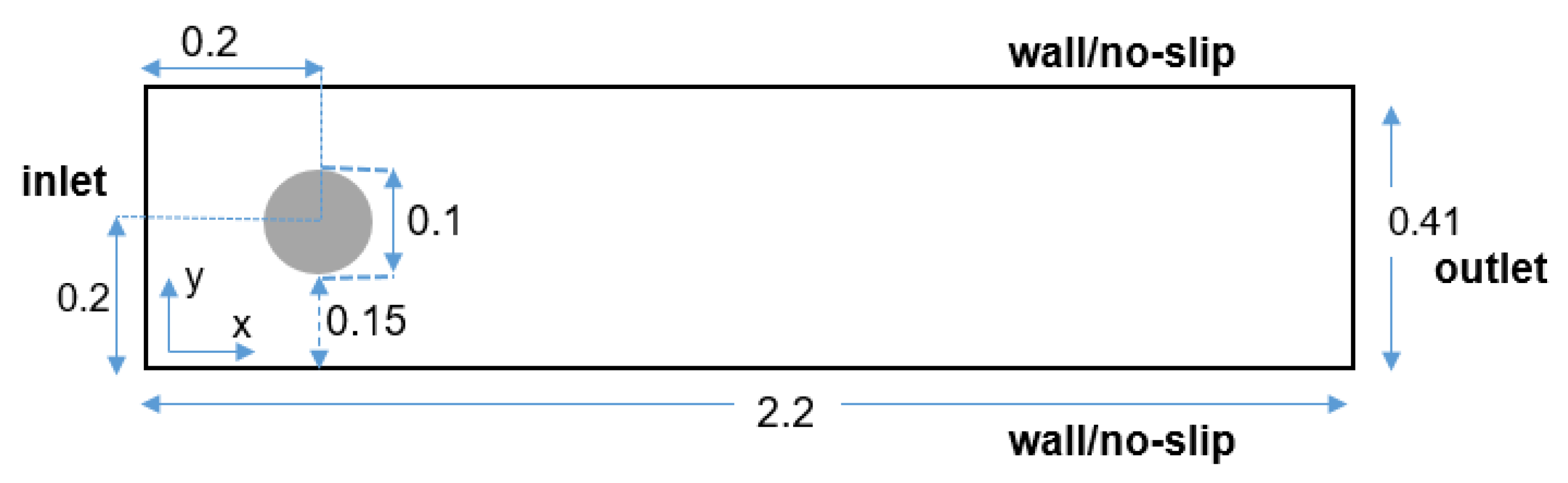
3.1.1. Random Shape Generation and Numerical Resolution of the Naiver–Stokes Equation

Numerical simulations were conducted to obtain the raw CFD dataset for our experiments.

The FEATool commercial code was used for the numerical simulations. The m-script programming language, used in the FEATool Multiphysics simulation toolbox, needs either MATLAB or the MATLAB Compiler Runtime (MCR) to run and interpret the source code.

A rectangular two-dimensional computational domain with a circular cylinder was considered in the numerical domain. In addition, other obstacles, such as triangles, rectangles, and polygons, were simulated in the same domain dimension as the cylinder obstacle. Figure 3 shows the benchmark problem for stationary flow and incompressible laminar flow around a cylinder, which was set up in rectangular 2D following [25,39].

The rectangular 2D domain dimensions were designed as follows; the width stream direction is 220 mm and the height direction perpendicular to flow is 41 mm. Grid computation and boundary setting are two essential components of CFD modeling. In our simulation, we used the triangle cell type for the grid type, with subdomain grid size 0.002 and growth rate 0.3. Therefore, the average cell count was approximately 35,000. For boundary setting, the left side of the 2D domain is the inlet and the right side is the outlet. No-slip conditions were assigned to the top and bottom sides as obstacle walls. In particular, inlet with velocity input ($u=u0$) had boundary coefficients ($u0=0.2$ and $v0=0$). Outflow with pressure output ($p=p0$) had boundary coefficient ($p0=0$). Walls with no-slip (u = 0) had no boundary coefficient. Furthermore, the boundary conditions were fixed with a constant density ($\rho$) set to the unity with a value of 1, viscosity ($\mu$) of 0.001, and F as the forcing term with 0 as the default value. A maximum velocity $u_{max}=0.3$ and a mean velocity $u_{mean}=\frac{2}{3}{u}_{max}=0.2$ were used, with a laminar flow Reynolds number $Re=\frac{\rho d{u}_{mean}}{\mu }=20$.

The equations for the mass and momentum of the incompressible 2D Navier–Stokes equations are given as follows:

$$\frac{\partial p}{\partial t}+\nabla ·\left(\rho u\right)=0$$

(1)

$$\frac{\partial }{\partial t}\left(\rho u\right)+\nabla ·\left(\rho u{v}^T\right)=-\nabla p+\nabla ·\tau +f$$

(2)

where the velocity field is denoted by u, density is denoted by $\rho$, the pressure field is denoted by p, the stress tensor is denoted by $\tau$, $v=\frac{\mu }{\rho 0}$ is the kinematic viscosity, and body forces (ex. gravity) are denoted by f.

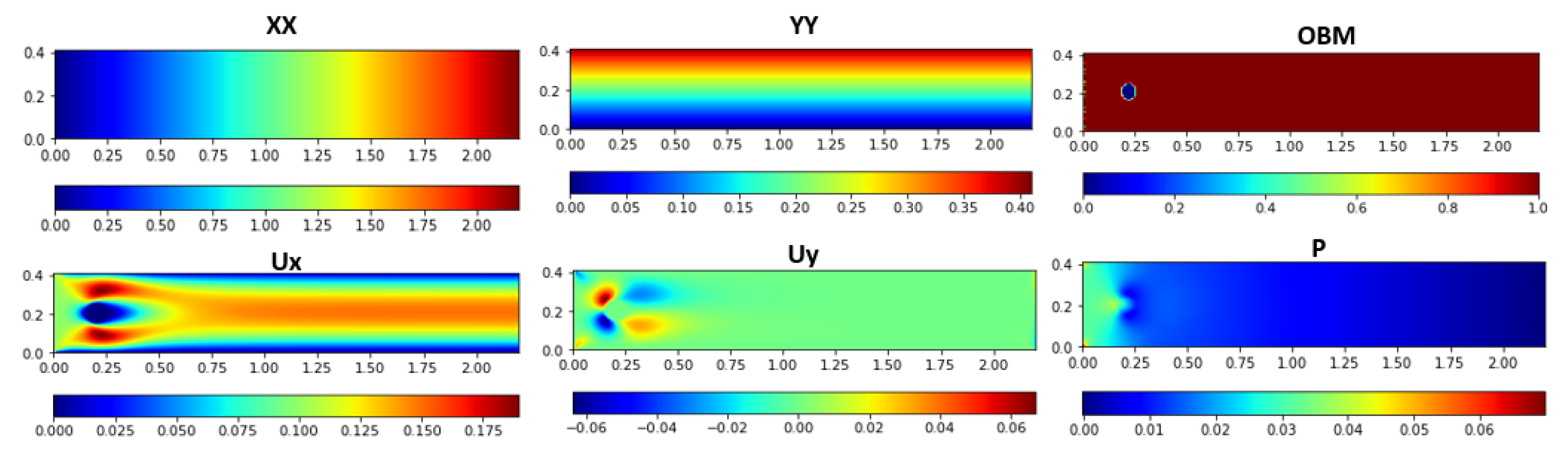
3.1.2. Learning Features Generation

The FEATool solver was used to generate a 2D laminar flow dataset around random obstacles with over 1000 samples. In FEATool, we used a shell script to write an automatic dataset with arbitrary geometry. The velocity and pressure fields were saved to the corresponding cell information for each computational grid. The following uses the CFD raw data to convert it into NumPy arrays as input and output features. The proposed interpolated grid algorithm converts the data so that it is easy to feed into deep networks for predicting fluid flows.

The raw data of velocities and pressure fields obtained by CFD solvers were projected onto these meshes by linear interpolation. Before providing the input fields to the learning network, the input features are reshaped to 2D $200\times 200$ arrays. After finishing the simulations, the raw CFD fluid flow field dataset with preprocessing was implemented following proposed Algorithm 1. Figure 4 presents the feature generated input ($XX,YY,OBM$) and interpolated learning output data ($Ux,Uy,P$) were generated using Algorithm 1.

The input and output learning features are generated using mesh-grid and grid-data computations under an interpolation process. First, a mesh grid is helpful to construct a well-defined 2D or even multi-dimensional space, which needs the ability to refer to each position in the space. In the first two channel inputs, we created a $m\times n$ Cartesian grid, with the x coordinate ranging from 1 to m and the y coordinate ranging from 1 to n. This means the ordered pairs of $(x,y)$ coordinates will begin from $(1,m)$ and go on until $(1,n)$. We depict two examples of 2D mesh-grid Numpy arrays below, $XX$ and $YY$, with $m\times m$ and $n\times n$ shapes, respectively.

$$X{X}_{m\times m}=\left[\begin{array}{ccccc}1& 2& 3& \cdots & m\\ 1& 2& 3& \cdots & m\\ 1& 2& 3& \cdots & m\\ ⋮& ⋮& ⋮& \ddots & ⋮\\ 1& 2& 3& \cdots & m\end{array}\right]$$

$$Y{Y}_{n\times n}=\left[\begin{array}{ccccc}1& 1& 1& \cdots & n\\ 2& 2& 2& \cdots & n\\ 3& 3& 3& \cdots & n\\ ⋮& ⋮& ⋮& \ddots & ⋮\\ n& n& n& \cdots & n\end{array}\right]$$

Hence, we can generally construct and visualize the mesh-grid structure ($MG$) following coordinate points of $XX$ and $YY$ as follows.

$$M{G}_{m\times n}=\left[\begin{array}{ccccc}11& 21& 31& \cdots & mn\\ 12& 22& 32& \cdots & mn\\ 13& 23& 33& \cdots & mn\\ ⋮& ⋮& ⋮& \ddots & ⋮\\ 1n& 2n& 3n& \cdots & mn\end{array}\right]$$

Algorithm 1: Interpolated Input and Output Features Generation

input: x-coordinate x,             y-coordinate y,             horizontal velocity u,             vertical velocity v,             pressure p,             width m,             height n output: 2D array of horizontal mesh-grid $XX$,               2D array of vertical mesh-grid $YY$,               object binary map $OBM$,               interpolated horizontal velocity $Ux$,               interpolated vertical velocity $Uy$,               interpolated pressure P 1 // Create two 1D array following x, y coordinates 2   $xg\leftarrow array\left[\right(min\left(x\right),max\left(x\right),m]$ 3   $yg\leftarrow array\left[\right(min\left(y\right),min\left(y\right),n\left)\right]$ 4 // Generate 2D numpy arrays are horizontal and vertical of mesh-grids using $xg$ and $yg$ 5   $XX,YY\leftarrow mesh\_grid(xg,yg)$ 6 // Generate obstacle binary mapping 7   $delta\_level\leftarrow 3$ 8   $delta\leftarrow arrange(delta\_level)$ 9   $x\_Index\leftarrow x\_Index+delta$ 10   $y\_Index\leftarrow y\_Index+delta$ 11   $x\_Index[x\_Index>=m]\leftarrow m-1$ 12   $y\_Index[y\_Index>=n]\leftarrow n-1$ 13   $binary\_Map[x\_Index,y\_Index]\leftarrow 1$ 14   $OBM\leftarrow transpose(binary\_Map)$ 15 // Generate output features 16   $Ux\leftarrow grid\_data\left(\right(x,y),u,(XX,YY\left)\right)$ 17   $Uy\leftarrow grid\_data\left(\right(x,y),v,(XX,YY\left)\right)$ 18   $P\leftarrow grid\_data\left(\right(x,y),p,(XX,YY\left)\right)$ 19 return $(XX,YY,OBM,Ux,Uy,P)$

   Second, grid data is used to interpolate a spatial set of data with z values. In this work, we interpolated three output features from raw data ($z=\{u,v,p\}$) in Equation (3).

$$Z=MG\left(\right(x,y),z)$$

(3)

In summary, the proposed Algorithm 1 comprises three main steps. The first step creates a mesh grid following the x, y coordinates obtained (pseudo-code presented in lines 2 to 3). The result of this step was used to interpolate the mesh grid in the next step. The second step generates two first channel inputs, $XX$ and $YY$, by interpolating the horizontal and vertical following the results of the first step (pseudo-code presented in line 5). The next step is to generate a third channel of the input, obstacle binary mapping (OBM) (pseudo-code presented in lines 7 to 14). The final step is to generate output features, including $Ux$, $Uy$, and P (pseudo-code presented in lines 16 to 18).

3.2. The Proposed CFD Based Deep U-Net Model

In this work, we developed our CFD model based on the U-Net architecture, which has been widely applied recently in computer vision tasks such as image translation, image recognition, etc. [31]. The conventional U-Net model has a bowtie structure that involves two network parts: an encoder and a decoder. The convolutional layers are used to translate the spatial information into extracted features. The spatial information will translate into the extracted features via the convolution layers. The U-Net model may include skipping connections to concatenate low-level features from the constructive path to the expansion path. In order to guarantee that the output layers are accessible for solution prediction, the U-Net architecture does indeed have skip links from the encoder to decoder networks. The architecture of the proposed U-Net is shown in Figure 1. Algorithm 2 presents the proposed learning model. The algorithm comprises three main steps. The first step is to create encoder and decoder networks during the training process (pseudo-code presented in lines 3 to 9). The second step is to predict the flow fields (pseudo-code presented in lines 10 to 12). The final step is to calculate the MSE losses of each relevant flow field (pseudo-code presented in lines 13 to 15).

Moreover, an essential part of the proposed learning model is the encoder–decoder. We reduced the data size by downsampling the stride convolution factor in the encoder network. With the growing number of feature channels, the network is allowed to extract increasing amounts of large-scale and abstract information. The encoding part takes the interpolated features, including $XX$, $YY$, and $OBM$. The encoder feature vectors $e^{enc}(XX,YY,OBM)$ can be formulated as:

$$e^{enc}(XX,YY,OBM)=Conv2d(XX,YY,OBM)$$

(4)

where $Conv2d(.)$ denotes the 2D convolution layer and a fully connected layer at the end. It is used to map the interpolated feature of the geometric vector representation.

With average pooling layers, the decoding network reduces the number of feature layers while increasing the spatial resolution. We may double the number of channels in each decoding block by employing skip connections to concatenate the channels from the encode section to the corresponding decode part. The deep U-Net model might consider the information of the low-level input channel via these skip connections while reconstructing a solution in the decode network part. Each network part uses a convolutional layer ($cv$), a batch normalization ($bn$) layer, and a non-linear activation function ($act$). Deconvolution operations are used to decode and transform high-level features encoded by the encoder network. The decoding process is given by the following formula:

$$d^{Ux,Uy,P}=Deconv2d\left(e^{enc}(XX,YY,OBM)\right)$$

(5)

where $d^{Ux,Uy,P}$ denotes three output channel predictions of the horizontal velocity ($Ux$), vertical velocity ($Uy$), and pressure (P). $Deconv2d(.)$ denotes multiple deconvolution layers using ReLU to map the extracted geometry representation vector to flow fields such as velocity and pressure.

In addition, we implemented our model using Python. We trained our model using an Adam optimizer and 1000 iterations of epochs because the training runs converged with the predicted accuracy. The learning rate, kernel size, and filter are a few additional significant hyperparameters of the adopted model discussed in the next section.

3.3. Model Evaluation and Optimization

One of the essential factors affecting the performance accuracy of the deep U-Net network is the hyperparameters. Therefore, finding suitable hyperparameters for the model can optimize the learning model and obtain good learning accuracy. Some hyperparameters are the number of hidden layers, learning rates, batch size, weight decay, filter, and kernel size. These values are described in detail in the following section. In addition, to evaluate the performance of the proposed model, we calculated the MSEs for each relevant flow field estimation as follows.

Algorithm 2: Deep U-Net-based CFD Prediction Model

The MSE of velocity $Ux$ calculation is as follows:

$$mse\_Ux=\sum _{i=1}^m{(Ux-Pre\_Ux)}^2$$

(6)

where $Ux$ is the actual horizontal velocity and $Pre\_Ux$ is the predicted horizontal velocity.

The MSE of velocity $Uy$ calculation is as follows:

$$mse\_Uy=\sum _{i=1}^m{(Uy-Pre\_Uy)}^2$$

(7)

where $Uy$ is the actual vertical velocity and $Pre\_Uy$ is the predicted vertical velocity.

The MSE of pressure P calculation is as follows:

$$mse\_P=\sum _{i=1}^m{(P-Pre\_P)}^2$$

(8)

where P denotes the actual pressure velocity and $Pre\_P$ is the predicted pressure velocity.

Hence, we calculate the total loss for the training and test processes as follows:

$$total\_Loss=mse\_Ux+mse\_Uy+mse\_P$$

(9)

4. Experimental Results and Discussion

4.1. Effectiveness of Hyper-Parameters

As described previously, model hyperparameters are essential for supporting deep networks to obtain convergence and enhance performance accuracy. In our experiment, we performed trial and error for some stable values by changing our learning models’ learning rate, batch size, and weight decay values. However, the model’s performance did not improve significantly when changing and adjusting these hyperparameter values. Hence, we determined the following suitable hyperparameters: a learning rate of 0.0001, a batch size of 64, and a weight decay of 0.005. However, we found that kernel sizes and filter hyperparameters influenced the proposed model, causing a significant reduction in the loss of flow prediction. We combined each of these hyperparameter values to determine the best combination. The effectiveness of both parameters is shown in

Table 1. Adjusting values of the important hyperparameters.

Kernel Size	Filter	Training Loss	Testing Loss	Ux’s MSE	Uy’s MSE	P’s MSE
	(4, 8, 16, 16)	8.043	8.585	4.740	3.465	0.379
5	(8, 16, 32, 32)	15.556	17.438	14.349	1.795	1.293
	(16, 32, 64, 64)	3.473	3.069	2.066	0.602	0.400
	(4, 8, 16, 16)	3.016	3.315	2.531	0.711	0.073
11	(8, 16, 32, 32)	3.016	3.315	2.531	0.711	0.073
	(16, 32, 64, 64)	0.309	0.452	0.404	0.033	0.014

. Table 1 shows that the suitable values of the kernel size and filter are 11 and (8, 16, 64, 64), as shown in the last bold row.

Furthermore, we visualized fluid flow prediction using our model. Figure 5 shows the CFD flow around the cylinder prediction results of the proposed method with the best parameters. In summary, the optimal hyperparameters were determined in this experiment. We then used these values to perform other experiments.

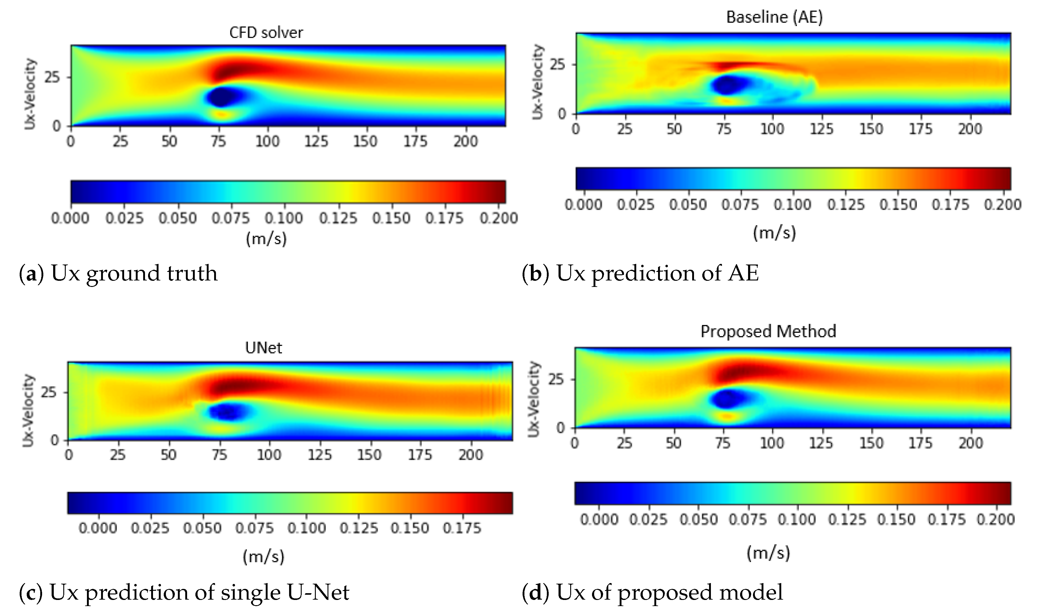
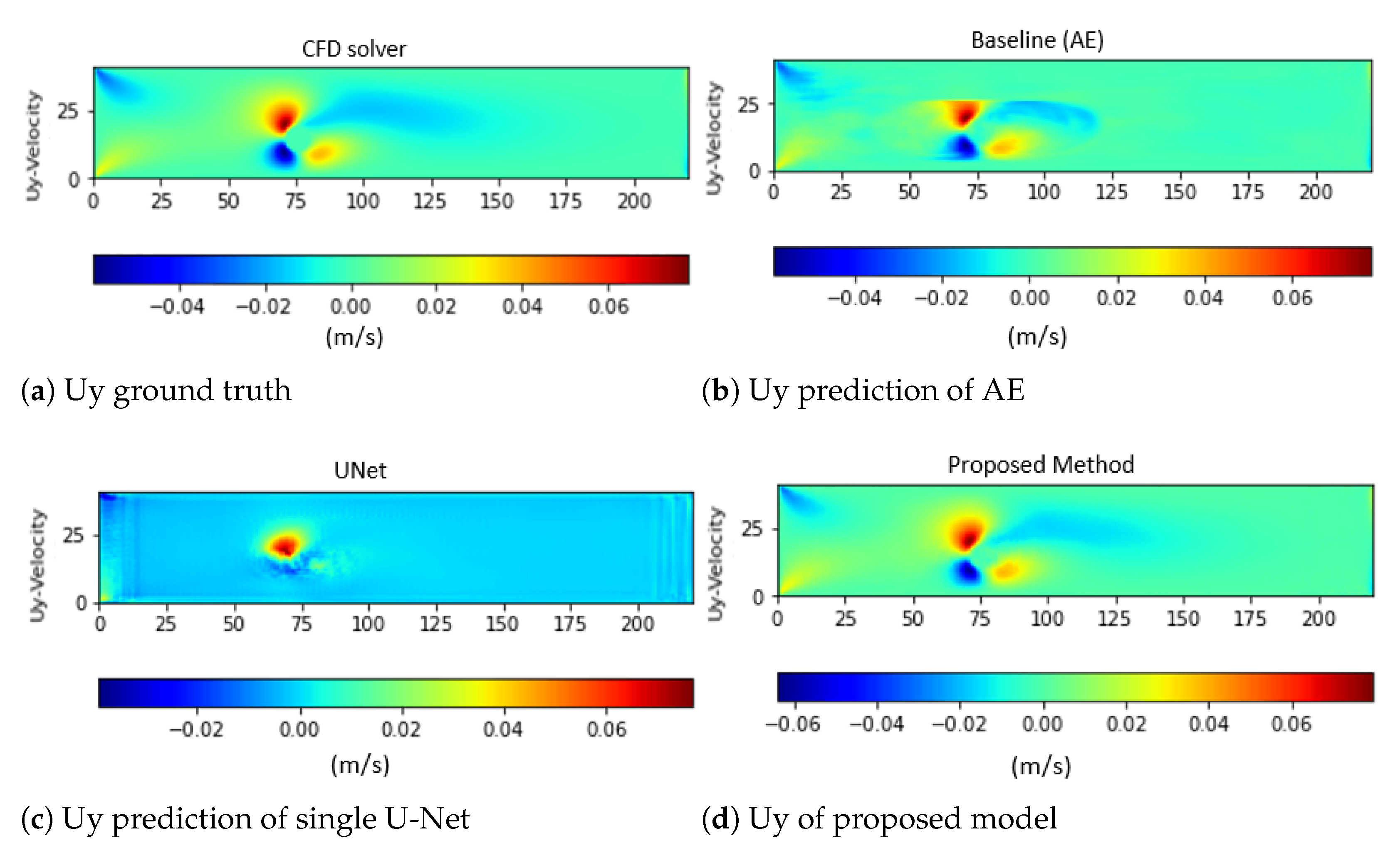
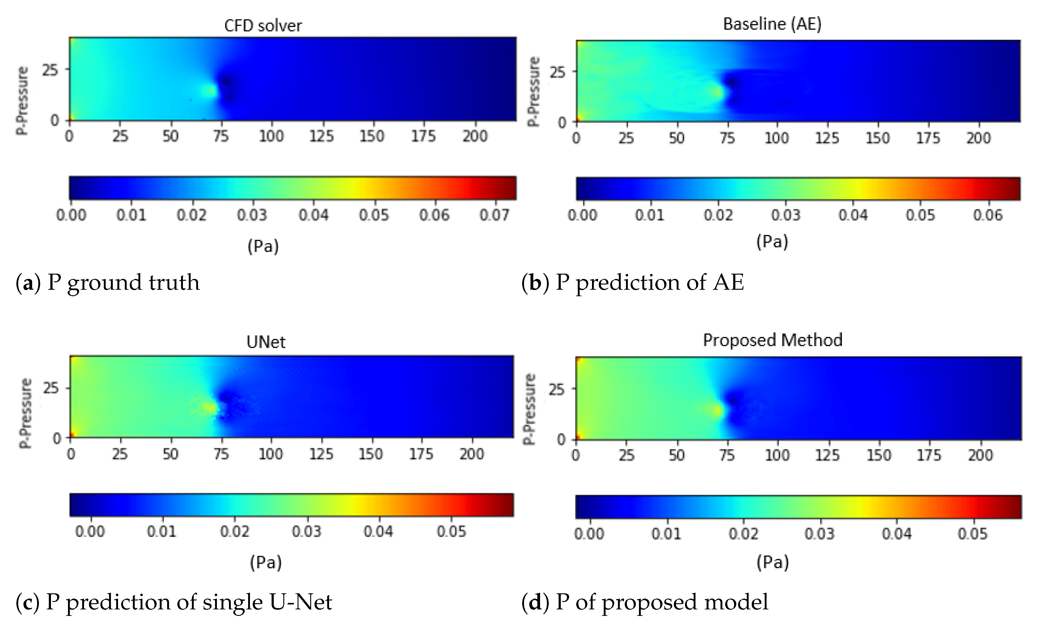
4.2. Performance Evaluation and Comparison to Other Deep Learning Models

In order to assess our model, we evaluated and depicted the MSE losses of the model during the training and testing processes, as shown in Figure 6. The loss graph demonstrates that the suggested strategy can maximize convergence while minimizing loss.

In addition, we experimented using the best hyperparameters determined over the flow predictions of other obstacles. The kernel value is 11 and the kernel size tuple is (16, 32, 64, 64), with the best performance obtained by the proposed method in the flow around cylinder prediction. Hence, we used these values for this experiment on other obstacles at different locations. Each obstacle estimation experiment is presented in

Table 2. Performance of the proposed method with different obstacles.

Obstacle	Train Loss	Test Loss	Ux’s MSE	Uy’s MSE	P’s MSE
Triangle	0.524	1.198	0.903	0.236	0.058
Rectangle	0.541	3.366	3.366	0.081	0.253
Pentagon	3.255	4.855	3.559	0.474	0.821

.

To compare the proposed method with other baseline models, we experimented with two models: AE and a single U-Net with one decoder over the same CFD dataset generated with cylinder, triangle, rectangle, and pentagon obstacles.

Table 3. Comparison of the performance results of the proposed method to other deep learning models.

Model	Training Loss	Testing Loss	Ux’s MSE	Uy’s MSE	P’s MSE
AE	11.183	11.183	12.688	1.125	1.408
Single U-Net	4.599	5.017	1.127	3.861	0.027
Proposed method	0.335	0.345	0.294	0.294	0.015

presents the results of the three approaches. The results show that our deep U-Net approach outperformed the other models (shown in the last bold row).

To illustrate the prediction performance of the proposed method, Figure 7, Figure 8 and Figure 9 show the prediction performance of the two related models and the proposed method. The results show that the proposed method is more accurate than other models. While the AE model obtained less accuracy on $Ux$ prediction (see Figure 7b) and the single U-Net model achieved the worst result for $Uy$ (see Figure 8c), the proposed method achieved the best accuracy for both $Ux$ and $Uy$ estimation (see Figure 7d and Figure 8d), as well as P prediction (see Figure 9d).

5. Conclusions

This paper presents a data-driven model for predicting steady-state flows with arbitrary obstacles in two-dimensional geometry, including cylinders, triangles, rectangles, and pentagons. In preprocessing the raw simulated CFD data, we generated novel interpolated grid features for the model learning data. The deep U-Net model was used to estimate 2D incompressible laminar flow over the generated interpolated feature data. The suggested model is more suited for coupling with numerical simulations, since the deep U-Net model operates directly on body-fitted triangular meshes of laminar flows surrounding the 2D obstacle dataset. According to the estimated results from the technique, the velocity and pressure fields of the issues with various obstacles measured by the proposed model agreed well with the CFD solver FEATool. Despite the different locations and obstacles, the network model can still provide a satisfactory reconstruction. The experimental findings provided accurate estimates of the pressure and velocity fields surrounding a pentagon, triangle, rectangle, and cylinder. In future work, we will consider and extend our work in different criteria experiments such as variations, perturbation, and Reynolds number value changes in simulation environments to evaluate our model performance and predict turbulence flow. Furthermore, we adapt and broaden our methodology to 3D simulated data in order to address pressure and temperature prediction challenges.

References

1. Portwood, G.D.; Mitra, P.P.; Ribeiro, M.D.; Nguyen, T.M.; Nadiga, B.T.; Saenz, J.A.; Chertkov, M.; Garg, A.; Anandkumar, A.; Dengel, A.; et al. Turbulence Forecasting via Neural Ode. 2019. Available online: https://arxiv.org/abs/1911.05180 (accessed on 22 February 2022).
2. Beck, A.D.; Flad, D.G.; Munz, C. Deep neural networks for data-driven turbulence models. CoRR 2018, abs/1806.04482. Available online: http://arxiv.org/abs/1806.04482 (accessed on 25 February 2022).
3. Ling, J.; Kurzawski, A.; Templeton, J. Reynolds averaged turbulence modelling using deep neural networks with embedded invariance. J. Fluid Mech. 2016, 807, 155–166. [Google Scholar] [CrossRef]
4. Tracey, B.D.; Duraisamy, K.; Alonso, J.J. A machine learning strategy to assist turbulence model development. In Proceedings of the 53rd AIAA Aerospace Sciences Meeting, Kissimmee, FL, USA, 5–9 January 2015. [Google Scholar]
5. Hagan, M.T.; Demuth, H.B.; Beale, M.H.; Jesús, O.D. Neural Network Design; PWS Publishing Co.: Cambridge, MA, USA, 2014. [Google Scholar]
6. Wang, Z.; Xiao, D.; Fang, F.; Govindan, R.; Pain, C.C.; Guo, Y. Model identification of reduced order fluid dynamics systems using deep learning. Int. Numer. Methods Fluids 2017, 86, 255–268. [Google Scholar] [CrossRef]
7. Fukami, K.; Fukagata, K.; Taira, K. Superresolution reconstruction of turbulent flows with machine learning. J. Fluid Mech. 2019, 870, 106–120. [Google Scholar] [CrossRef]
8. Fresca, S.; Dedè, L.; Manzoni, A. A comprehensive deep learning-based approach to reduced order modeling of nonlinear time-dependent parametrized PDEs. J. Sci. Comput. 2021, 87, 61. [Google Scholar] [CrossRef]
9. Fresca, S.; Manzoni, A. POD-DL-ROM: Enhancing deep learning-based reduced order models for nonlinear parametrized PDEs by proper orthogonal decomposition. Comput. Methods Appl. Mech. Eng. 2022, 388, 114181. [Google Scholar] [CrossRef]
10. Fresca, S.; Manzoni, A. Real-Time Simulation of Parameter-Dependent Fluid Flows through Deep Learning-Based Reduced Order Models. Fluids 2021, 6, 259. [Google Scholar] [CrossRef]
11. Pant, P.; Doshi, R.; Bahl, P.; Barati, F.A. Deep learning for reduced order modelling and efficient temporal evolution of fluid simulations. Phys. Fluids 2021, 33, 107101. [Google Scholar] [CrossRef]
12. Kang, H.; Tian, Z.; Chen, G.; Li, L.; Wang, T. Application of POD reduced-order algorithm on data-driven modeling of rod bundle. Nucl. Eng. Technol. 2022, 54, 36–48. [Google Scholar] [CrossRef]
13. Gao, H.; Sun, L.; Wang, J.-X. Phygeonet: Physicsinformed geometry-adaptive convolutional neural networks for solving parametric pdes on irregular domain. J. Comput. Phys. 2021, 428, 110079. [Google Scholar] [CrossRef]
14. San, O.; Maulik, R.; Ahmed, M. An artificial neural network framework for reduced order modeling of transient flows. Commun. Nonlinear Sci. Numer. Simul. 2019, 77, 271–287. Available online: https://www.sciencedirect.com/science/article/pii/S1007570419301364 (accessed on 18 March 2022). [CrossRef] [Green Version]
15. Sekar, V.; Khoo, B.C. Fast flow field prediction over airfoils using deep learning approach. Phys. Fluids 2019, 31, 057103. [Google Scholar] [CrossRef]
16. Jin, X.; Cheng, P.; Chen, W.-L.; Li, H. Prediction model of velocity field around circular cylinder over various Reynolds numbers by fusion convolutional neural networks based on pressure on the cylinder. Phys. Fluids 2018, 30, 047105. [Google Scholar] [CrossRef]
17. Guo, X.; Li, W.; Iorio, F. Convolutional Neural Networks for Steady Flow Approximation; ser. KDD ’16; Association for Computing Machinery: New York, NY, USA, 2016; pp. 481–490. [Google Scholar] [CrossRef]
18. Ribeiro, M.D.; Rehman, A.; Ahmed, S.; Dengel, A. Deepcfd: Efficient Steady-State Laminar Flow Approximation with Deep Convolutional Neural Networks. 2020. Available online: https://arxiv.org/abs/2004.08826 (accessed on 13 March 2022).
19. Featool Multiphysics. FEATool Multiphysics. 2013–2022. Available online: https://www.featool.com/doc/quickstart.html (accessed on 12 January 2022).
20. Sarghini, F.; de Felice, G.; Santini, S. Neural networks based subgrid scale modeling in large eddy simulations. Comput. Fluids 2003, 32, 97–108. Available online: https://www.sciencedirect.com/science/article/pii/S0045793001000986 (accessed on 16 March 2022). [CrossRef]
21. Lee, S.; You, D. Data-driven prediction of unsteady flow over a circular cylinder using deep learning. J. Fluid Mech. 2019, 879, 217–254. [Google Scholar] [CrossRef]
22. Kashefi, A.; Rempe, D.; Guibas, L.J. A point-cloud deep learning framework for prediction of fluid flow fields on irregular geometries. Phys. Fluids 2021, 33, 027104. [Google Scholar] [CrossRef]
23. Lui, H.F.S.; Wolf, W.R. Construction of reducedorder models for fluid flows using deep feedforward neural networks. J. Fluid Mech. 2019, 872, 963–994. [Google Scholar] [CrossRef]
24. Tompson, J.; Schlachter, K.; Sprechmann, P.; Perlin, K. Accelerating Eulerian Fluid Simulation with Convolutional Networks. 2016. Available online: https://arxiv.org/abs/1607.03597 (accessed on 28 March 2022).
25. Ribeiro, M.D.; Portwood, G.D.; Mitra, P.; Nyugen, T.M.; Nadiga, B.T.; Chertkov, M.; Anandkumar, A.; Schmidt, D.P.; Team, N.; Team, U.; et al. A data-driven approach to modeling turbulent decay at non-asymptotic Reynolds numbers. In Proceedings of the APS Division of Fluid Dynamics Meeting Abstracts 2019, Provided by the SAO/NASA Astrophysics Data System, Seattle, WA, USA, 23–26 November 2019; p. G16.002. [Google Scholar]
26. Gupta, S.; Girshick, R.; Arbeláez, P.; Malik, J. Learning Rich Features from Rgb-D Images for Object Detection and Segmentation. 2014. Available online: https://arxiv.org/abs/1407.5736 (accessed on 27 March 2022).
27. Socher, R.; Huval, B.; Bhat, B.; Manning, C.D.; Ng, A.Y. Convolutional-recursive deep learning for 3d object classification. In Proceedings of the 25th International Conference on Neural Information Processing Systems, Harrahs and Harveys, NV, USA, 3–8 December 2012; ser. NIPS’12. Curran Associates Inc.: Red Hook, NY, USA, 2012; Volume 1, pp. 656–664. [Google Scholar]
28. Georgiou, T.; Schmitt, S.; Olhofer, M.; Liu, Y.; Bäck, T.; Lew, M. Learning fluid flows. In Proceedings of the 2018 International Joint Conference on Neural Networks (IJCNN), Rio de Janeiro, Brazil, 8–13 July 2018; pp. 1–8. [Google Scholar]
29. Zhang, Y.; Sung, W.-J.; Mavris, D. Application of Convolutional Neural Network to Predict Airfoil Lift coefficient. 2017. Available online: https://arxiv.org/abs/1712.10082 (accessed on 16 March 2022).
30. Viquerat, J.; Hachem, E. A supervised neural 10 VOLUME, 2021Author Le et al.: Towards Incompressible Laminar Flow Estimation Based on Interpolated Feature Generation and Deep Learning network for drag prediction of arbitrary 2d shapes in laminar flows at low reynolds number. Comput. Fluids 2020, 210, 104645. Available online: https://www.sciencedirect.com/science/article/pii/S0045793020302164 (accessed on 2 April 2022). [CrossRef]
31. Ronneberger, O.; Fischer, P.; Brox, T. Unet: Convolutional Networks for Biomedical Image Segmentation. 2015. Available online: https://arxiv.org/abs/1505.04597 (accessed on 4 April 2022).
32. Thuerey, N.; Weißenow, K.; Prantl, L.; Hu, X. Deep learning methods for reynolds-averaged navier–stokes simulations of airfoil flows. AIAA J. 2020, 58, 25–36. [Google Scholar] [CrossRef]
33. Kamrava, S.; Tahmasebi, P.; Sahimi, M. Physics and image-based prediction of fluid flow and transport in complex porous membranes and materials by deep learning. J. Membr. Sci. 2021, 622, 119050. [Google Scholar] [CrossRef]
34. Wang, Y.D.; Chung, T.; Armstrong, R.T.; Mostaghimi, P. Ml-lbm: Machine Learning Aided Flow Simulation in Porous Media. 2020. Available online: https://arxiv.org/abs/2004.11675 (accessed on 5 March 2022).
35. Chen, J.; Viquerat, J.; Heymes, F.; Hachem, E. A Twin-Decoder Structure for Incompressible Laminar Flow Reconstruction with Uncertainty Estimation around 2D Obstacles. 2021. Available online: https://arxiv.org/abs/2104.03619 (accessed on 7 April 2022).
36. Peng, J.-Z.; Liu, X.; Aubry, N.; Chen, Z.; Wu, W.-T. Data-driven modeling of geometryadaptive steady heat conduction based on convolutional neural networks. Case Stud. Thermal Eng. 2021, 28, 101651. Available online: https://www.sciencedirect.com/science/article/pii/S2214157X21008145 (accessed on 10 April 2022). [CrossRef]
37. Eichinger, M.; Heinlein, A.; Klawonn, A. Stationary flow predictions using convolutional neural networks. In ENUMATH, Lecture Notes in Computational Science and Engineering; Springer: Berlin/Heidelberg, Germany, 2019; Volume 139. [Google Scholar]
38. Li, K.; Li, H.; Li, S.; Chen, Z. Fully convolutional neural network prediction method for aerostatic performance of bluff bodies based on consistent shape description. Appl. Sci. 2022, 12, 3147. [Google Scholar] [CrossRef]
39. Nabh, G. On High Order Methods for the Stationary Incompressible Navier-Stokes Equations, ser. Interdisziplinäres Zentrum für Wissenschaftliches Rechnen der Universität Heidelberg. IWR. 1998. Available online: https://books.google.co.kr/books?id=cx4-HAAACAAJ (accessed on 15 April 2022).
Figure 1. The proposed network architecture.
Sustainability 14 11996 g001
Figure 2. Data collection from CFD solver.
Sustainability 14 11996 g002
Figure 3. Example of flow around cylinder simulation.
Sustainability 14 11996 g003
Figure 4. Examples of learning data features generation. The first row is the input feature generated (XX, YY, and OBM). The second row is the output feature generated (Ux, Uy, P).
Sustainability 14 11996 g004
Figure 5. CFD flow fields (velocities and pressure) prediction obtained. The first column is ground truth, the second column is CFD flow fields prediction, and the third column is MSE loss. (a) Ux velocity; (b) Uy velocity; (c) P pressure.
Sustainability 14 11996 g005
Figure 6. MSE loss graphs for training and testing processes.
Sustainability 14 11996 g006
Figure 7. Comparison of velocity (Ux) estimation performance of the proposed method to other related models.
Sustainability 14 11996 g007
Figure 8. Comparison of the proposed method’s velocity (Uy) estimation performance to other related models.
Sustainability 14 11996 g008
Figure 9. Comparison of the proposed method’s pressure (P) estimation performance to other related models.
Sustainability 14 11996 g009