Article

The Role of Digital Soil Information in Assisting Precision Soil Management

1
School of Agriculture, Food and Wine, The University of Adelaide, Adelaide, SA 5005, Australia
2
Department of Soil Resources and Watershed Management, Wollega University, Shambu P.O. Box 38, Ethiopia
3
Organic Recycling Institute (Suzhou), China Agricultural University, Wuzhong District, Suzhou 215128, China
4
Faculty of Process and Environmental Engineering, Lodz University of Technology, Wolczanska Str. 213, 90-924 Lodz, Poland
5
Department of Botany and Microbiology, College of Science, King Saud University, Riyadh 11451, Saudi Arabia
6
Soil Fertility Improvement and Problematic Soil Management Research Team, Nekemte Soil Research Center, Oromia Agricultural Research Institute, Nekemte P.O. Box 81265, Ethiopia
7
Department of Research and Scientific, International Fertilizer Development Center, Addis Ababa P.O. Box 5689, Ethiopia
8
Faculty of Security Engineering and Civil Protection, The Main School of Fire Service, Slowackiego Street 52/54, 01-629 Warsaw, Poland
9
College of Plant Sciences and Technology, Huazhong Agricultural University, Wuhan 430070, China
*
Authors to whom correspondence should be addressed.
Sustainability 2022, 14(18), 11710; https://doi.org/10.3390/su141811710
Submission received: 9 August 2022 / Revised: 16 September 2022 / Accepted: 16 September 2022 / Published: 18 September 2022

Abstract

:
Soil information is the basis for the site-specific management of soils. The study aimed to digitize soil information and classify it into soil mapping units (SMUs) using geostatistics. The study area was grouped into 12 SMUs, or management zones. The pH of the soils ranged from 7.3 in SMU2 to 8.6 in SMU5. Most SMUs exhibited low total nitrogen (TN) that could be attributed to very low soil organic carbon (SOC) in the soils. Available phosphorus (AvP) was very low in all the mapping units. The exchangeable K varied between 0.12 cmol(+) kg−1 (SMU7) and 0.95 cmol(+) kg−1 (SMU10). SMU12 was identified as marginally sodic and at a high risk of developing severe alkalinity unless possible management measures are implemented. Our findings show that a lack of soil information causes an imbalance between soil requirements and external nutrient inputs, negatively affecting crop production. Therefore, high-resolution digital soil information can assist the site-specific application of soil nutrients and amendments based on spatial variability in line with soil requirements.

1. Introduction

To meet global food demand, higher crop production in developed and developing countries has to come from agricultural intensification [1,2]. However, some of the major constraints reducing agricultural yields are soil nutrient deficiencies, suboptimal management of resources, and limited information on soil nutrient availability [3]. Digital soil fertility information is very scarce in developing countries, and land managers are largely unaware of this technology [4,5]. In traditional farming systems, inputs such as fertilizers are applied uniformly for the whole field, although the availability of the nutrients in soils is not homogeneous. For this reason, the application of uniform fertilizer rates to a non-homogeneous area of land based on soil data obtained from a few points results in low crop yield, economic loss, and land degradation [4,6]. This suggests that a lack of up-to-date soil information containing high-resolution soil conditions is one of the major impediments to agricultural intensification in developing countries and anywhere across the world. As a result, knowledge of the spatial heterogeneity of soil properties at the farmland/landscape scale is critical for determining crop production constraints and implementing appropriate soil management practices [7,8].
Though the harmonized soil polygon map of Africa, known as the ‘Soil Atlas of Africa’ recently produced by [9] at scales varying between 1:1M and 1:5M can be useful, it is not at a required resolution to be applied at the farm level. Soil information maps can be produced using a wide range of statistical and mathematical approaches such as machine learning, data mining, regressions, deep learning, and geostatistics [10,11,12,13]. Geostatistics are used to generate maps and thus to estimate the value of soil properties for unsampled sites based on those of sampled sites [14]. Digital soil maps can display the spatial variability of soil nutrients at a finer resolution, assisting landowners in identifying high and low nutrient distributions within their fields [15,16]. As a result, there is a need to generate digital soil information to develop precise nutrient recommendations [17,18,19] and ultimately to mechanize the traditional agricultural systems in developing countries such as Africa [5].
In this regard, digital soil information helps to classify soils into management zones that aid spatially targeted nutrient advisory works, thereby reducing under and/or over-application of nutrients and amendments [13,20]. In addition to its agronomic efficiency, it has also economic benefits in terms of saving farmers’ money through more efficient use of fertilizers. Therefore, the study was aimed to map soils at a finer resolution of 1:10,000, to produce management zones, and to provide soil information for precise nutrient management.

2. Materials and Methods
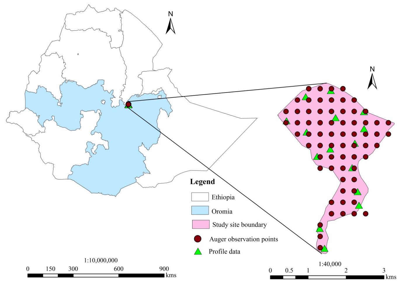
2.1. Study Site

The research was carried out in the Gololcha district of the west Hararghe of Oromia region in Ethiopia. It is located between 8°53′33″ and 8°56′02″ N latitudes and 40°18′30″ and 40°53′33″ E longitudes, at an elevation of 1150 to 1240 m above sea level (Figure 1). The study area covers 489.96 ha of land, excluding rock surfaces. About 54% of the study site comprised of gentle slope (4–8%) and moderate to steep slope classes (8–15%). The remaining portion of the site showed level land (0–4%). Communities residing in the study area practiced the mixed farming system. Cereals (maize, and sorghum), fruits (banana and avocado), stimulants (coffee and chat), and oil crops (groundnuts, Niger seed, and haricot bean) are the main crops grown in the area.

2.2. Research Design and Procedures

2.2.1. Pre-Field Survey

This stage involved office activities such as the preparation of a base map to aid in land surveying. The base maps of landform and land use for the study boundary were produced by overlaying a 30 m resolution Landsat ETM+ and Google Earth image using ArcGIS 10.3 software. The slope classes were generated from a 30 m resolution digital elevation model (DEM) using Global Mapper 30.2 software. Hereafter, the boundary of the study site (i.e., arable land) was delineated from the base maps produced for slope, landform, and land use. The location and number of predefined auger observation points that aided field survey activities were then estimated using a 300 m × 300 m grid size and distributed on the 1:10,000 scale base map. The grid points were encoded into the Global Positioning System (GPS) and used to locate points for soil characterization and sampling activities during the field survey.

2.2.2. Field Survey

First, augering points in the field were identified using predefined sampling points on the map (Figure 1). The soil was then described and sampled for 68 auger observation points. Different landscape variables, for example, Universal Traverse Mercator (UTM) coordinates, elevation, erosion status, slope steepness, and surface drainage conditions were characterized at each auger observation point following [21] guidelines. Furthermore, various soil properties, i.e., soil depth and textural classes, were investigated at every auger observation site.
The slope, soil depth, and texture were used as covariates to categorize the soil samples at the study site into various soil mapping units (SMUs). By combining the data of all coordinates derived from the auger observation points and the mini pits, the entire study site was classified into 12 SMUs. This was accomplished by overlaying maps of the slope, soil depth, and texture to create soil units with similar characteristics. Later on, soil samples were collected from 0–20 cm depth to estimate the soil fertility of the land units. For each grid point, 12 subsamples were collected and mixed to form a composite sample. As a result, a total of 68 composite samples were collected from all the SMUs in the study site.

2.2.3. Post-Field Survey

The post-field survey work focused on soil sample preparation, soil analysis, digital mapping, grouping farmlands into management zones, and placing management recommendations. The final soil map with SMUs was created at a scale of 1:10,000 with ArcGIS 10.3 software. Then, the boundaries of the SMUs or management zones were coded into GPS and navigated on the ground. Consequently, the management zones were used to advise on nutrient recommendations and other soil management practices. Farmers and land users residing in similar management zones were advised to follow the harmonized management decisions.

2.3. Sample Preparation and Analysis

Soil samples were air dried and then ground to pass through a 2 mm sieve size. Selected soil physical and chemical properties were tested based on standard methods. The percentage of sand, silt, and clay in the soils was determined by the modified sedimentation hydrometer method [22]. Soil pH and electrical conductivity (EC) was estimated using a suspension of 1:1.25 soil to water ratio as outlined by [23]. The soil organic carbon was measured using the oxidation method of Walkley and Black [24]. Total nitrogen (TN) was determined by the Kjeldahl method [25]. Available phosphorus (AvP) was determined by the Olsen method [23]. Cation exchange capacity (CEC) was determined by using the 1M ammonium acetate (pH 7) extraction method [23]. The similar ammonium acetate leachate was used to measure the amounts of exchangeable Ca2+ and Mg2+ using an Atomic Absorption Spectrophotometer (AAS), as well as exchangeable K+ and Na+ with a flame photometer.

2.4. Statistical Data Analysis

Statistical analyses including descriptive statistics and principal component analysis (PCA) were carried out using XLSTAT 2015 (version 4.01) software. Geostatistical analysis was performed using ArcGIS 10.3 software. The Pearson correlation coefficient was used to evaluate the relationship between soil variables at a significance level of 0.05.

3. Results

3.1. Descriptive Statistics for the Entire Study Site

Table 1 presents a statistical summary of the measured values for the soil properties representing the entire study area. In this section, the soil properties were interpreted by considering the whole study area as a single unit. The pH of the soil ranged from 7.3 to 8.7, with a mean of 7.9 and a standard deviation of 0.4, indicating a cluster of values close to the mean. The pH values had a skewness coefficient of 0.6 and its distribution was moderately skewed to the right. The minimum and maximum values for total N were 0.08% and 0.24%, respectively. Total N showed a skewness coefficient of 0.21. The values of exchangeable Mg, TN, OC, PBS, Ca:Mg ratio, and K:Mg ratio are fairly symmetrical, with skewness values ranging between -0.5 and 0.5 (Table 1). The AvP content of the soils across the entire study area ranged from 1.14 to 5.34 ppm, with a mean value of 2.69 ppm. The mean percent base saturation (PBS) of the soils was 86.30%, varying between 73.22 and 94.16%.
The first five principal components (PC) accounted for 85.31% (PC1 = 35.29%, PC2 = 16.83%, PC3 = 12.75%, PC4 = 12.18%, and PC5 = 8.27%) of the total variance that best explains the data set (Table 2). The first five components showed eigenvalues greater than 1 (Table 2). As a result, the total variances of the PCs with eigenvalues greater than 1 were used to explore the variability of the data.

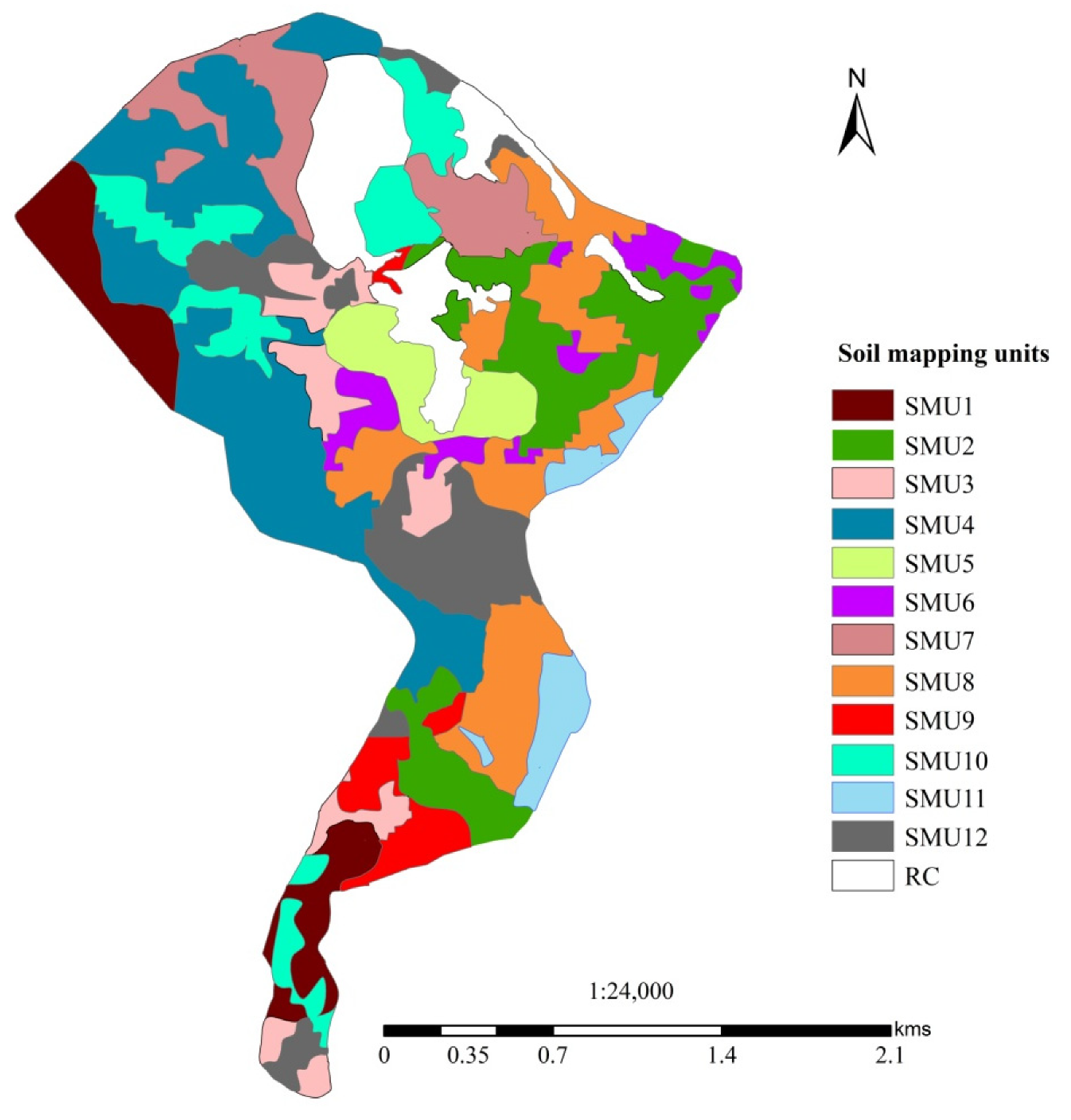
3.2. Extent and Distribution of Soil Mapping Units

In the study area, 12 SMUs were identified (Table 3). SMU4 occupied the largest portion of the study area (20.75%), whereas SMU11 occupied the smallest portion (3.35%) compared with other SMUs. The mapping units demonstrated a range of slope classes, soil depth, and soil texture (Table 3). The SMU1 was formed on a 0–2% slope with a very deep (>150 cm) clay soil throughout the profile. The SMU2 was developed on a 0–2% slope with a moderately deep profile (50–100 cm). However, the SMU5, SMU6, SMU7, and SMU12 were all developed on a slope of 4–6% (Table 3) but differ in their soil depth. The SMU8, SMU9, and SMU10 were all identified on a 6–8% slope, exhibiting soil depth ranging between 100 cm and 150 cm. Exceptionally, the SMU11 occurred on steep slopes of 8–15% with shallow soils (<50 cm).
The distribution of SMUs across the study site was shown in Figure 2. Cambisols differing in soil series and qualifiers were identified in SMU2, SMU5, SMU6, SMU8, SMU9, and SMU12. The Cambisols occupied 41.85% of the total study area. They were formed on recent alluvial deposits. On the other hand, the soils of SMU1, SMU3, SMU4, and SMU7 were Vertisols. Accounting for 37.6% of the entire study area, Vertisols were distributed in areas with slopes below 6%. The remaining SMU10 and SMU11 were occupied by Fluvisols and Leptosols, respectively. The Fluvisols had clay loam throughout the soil profile, indicating that there was little profile development. However, the Leptosols exhibited very shallow soils, which could be attributed to their formation on steep slopes of 8–16% that were prone to erosion. The SMUs on the current soil map were, in general, considered as management zones that could be used to harmonize soil management practices.

3.3. Soil Nutrients and Salinity Problems across the Mapping Units

The concentration of soil nutrients varies from soil unit to soil unit. The average pH ranged from 7.3 (SMU2) to 8.6 (SMU5) (Table 4). All land units have a pH in the alkaline range. The mean TN in the SMU7 ranged from 0.1 to 0.17% in the SMU11. The mean AvP in all SMUs was very low, making it the major limiting nutrient in the study area. All of the SMUs had a very low soil OC (2%), resulting in low TN in the soils; this is because the main source of TN in soils is organic matter.
The mean exchangeable Na content of the soils ranged from low (0.25 cmol(+) kg−1) in SMU2 to very high (3.95 cmol(+) kg−1) in SMU12 (Table 4). However, the rest of the SMUs had moderate to high exchangeable Na. The mean value of exchangeable K ranged from 0.12 cmol(+) kg−1 in SMU7 to 0.95 cmol(+) kg−1 in SMU10. Except for SMU10, which exhibited a high exchangeable K, the remaining SMUs had very low to moderate exchangeable K. This demonstrates that, unlike SMU10, the entire mapping unit requires the application of K fertilizers. The overall mean value of divalent cations (Ca and Mg) in the SMUs was high to very high, forming calcareous soils. In the entire SMUs, the percent base saturation (PBS) was consistently greater than 80%. The balance between exchangeable cations also affects the fertility of soils. Our findings show that the mean Ca:Mg ratio ranged from 2.75 in SMU12 to 7.11 in SMU2, and almost all the mapping units had a low K:Mg ratio (Table 4). Standard deviation (SD) was higher than or equal to the mean for K:Mg ratio in SMUs 3, 4, 5, 6, 8, 9, 11, and 12 (Table 4). This shows that the data for the K:Mg ratio was not normally distributed. In such cases, the mean cannot provide a good measure of central tendency, indicating that K:Mg ratios vary greatly across the landscape.
The mean electrical conductivity (EC) of the soils ranged from 0.20 mS cm−1 in SMU2 to 2.05 mS cm−1 in SMU12. The SD was greater than or equal to the mean for EC in SMUs 4, 6, 8, and 12 (Table 4). This demonstrates that the data for EC was not normally distributed, similar to the K:Mg ratio. Except for SMU12, which was classified as slightly saline (ECe 2–4 mS m−1), all SMUs were currently non-saline. This suggests that farmlands in SMU12 require reclamation before the problem becomes severe. Other SMUs that are not currently saline are also susceptible to developing salinity issues, necessitating regular soil testing and monitoring.
Despite the spatial heterogeneity of soils across the study site, our survey results showed that farmers both inside and outside the study border historically similarly managed their farm plots. For example, they were applying nutrients to all SMUs at blanket fertilizer rates of 150 kg ha−1 DAP and 100 kg ha−1 UREA for all the SMUs. This apparently led to considerable yield gaps in the study area.

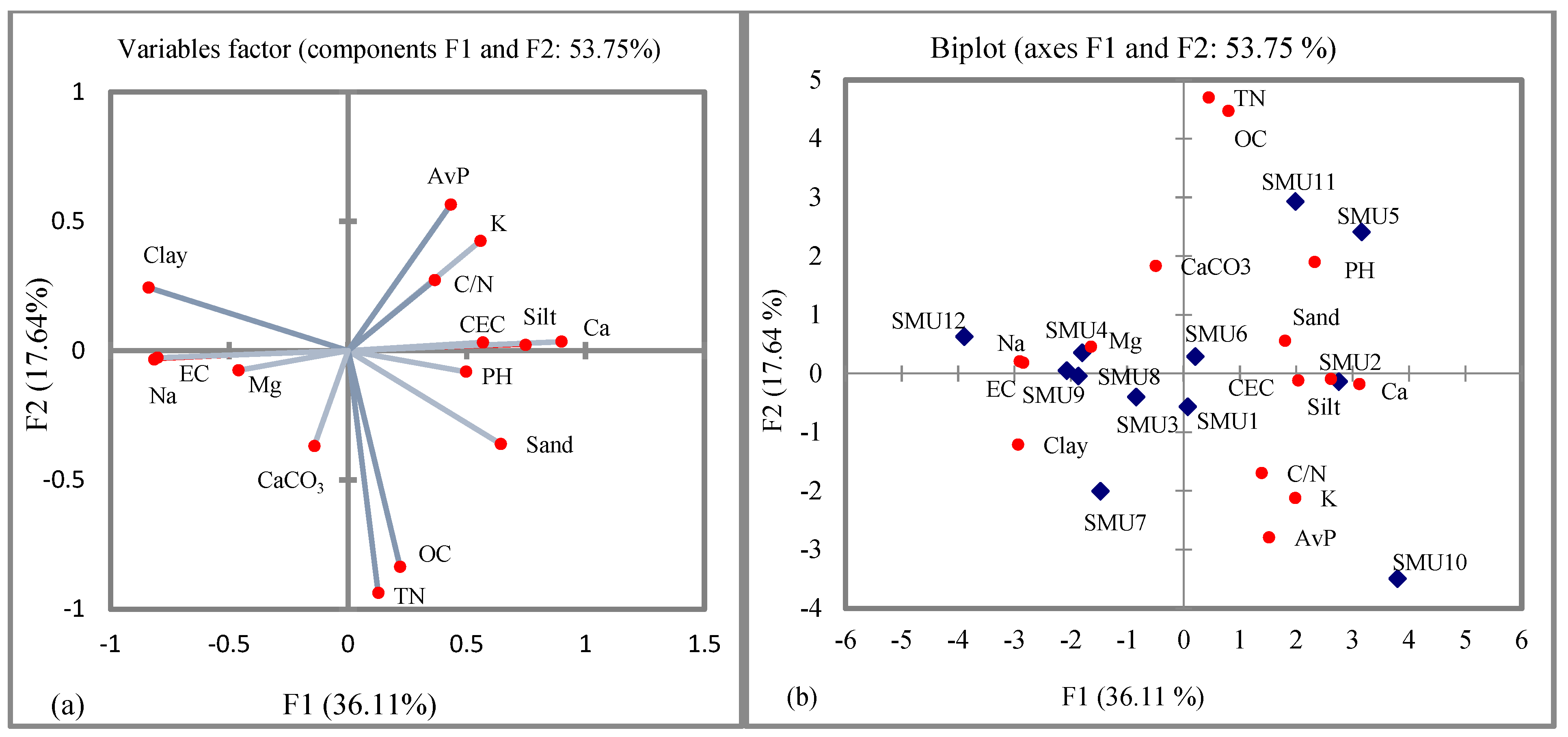
3.4. The Relationship between Soil Properties

A factor plot describing the first two components was used to illustrate the relationship between soil properties (Figure 3a). As observed from the magnitude and direction of correlation lines (Figure 3a), there was a good correlation between TN and OC; Na and EC; AvP and exchangeable K; pH and CEC; silt and Ca. Close correlation lines between TN and soil OC shows that OC was the primary source of TN in the soils. On the factor plot, variables positioned in a straight line or at right angles did not correlate positively. For instance, AvP did not correlate with OC, suggesting that mineral rocks rather than organic matter could be the main source of AvP in the soils of the study site. Similarly, there was a poor correlation between AvP and exchangeable Mg. Figure 3b demonstrates that SMU12 is distinct from other SMUs in terms of its high EC and exchangeable Na, whereas SMU5 stands out for having a comparatively high pH value. In general, the grouping of SMUs based on the magnitude of soil parameters (Figure 3b) can be used for site-specific management decisions.

4. Discussion

4.1. Management Zones for Spatially Targeted Nutrient Management

One of the main causes of low crop production in the study area is a homogeneous soil management practice across varying soils. According to [26], soil management interventions that are not tailored to the specific soil conditions result in lower yields and profitability. This problem is particularly acute in areas where soil information is scarce [27,28]. Uniform management recommendations for spatially heterogeneous soils lead to low agronomic efficiency because it does not consider the site-specific needs of the soils. As a result, a management zone approach that considers the spatial variability of soil requirements is a good option for optimum nutrient management and improved crop production.
The management zone approach divides farmland into mapping units based on site-specific soil requirements. In this study, soils were divided into management zones using the grid sampling approach. Using this method, it is possible to determine how soil potentials and constraints vary between management zones and to target fertilizer sources and rates according to the critical levels of soil nutrients in each SMU. For example, the total N classifications based on [29,30] ratings showed that SMU5 and SMU11 exhibited optimum while the rest of the SMUs contained low TN. As a result, all SMUs require the application of varying amounts of N fertilizers depending on the critical values of TN in each SMU. Since the soils in all SMUs have a pH higher than 7, it is advisable to apply ammonium-containing fertilizers to slow further alkalinization processes in the soils. The low TN in the soils could be due to very low soil OC (SOC). The low to very low SOC in the study site is in turn caused by exhaustive tillage practices and low residue incorporation into the soils [31,32]. As a result, organic amendments that can supply OC and N including compost, vermicompost, manure, biochar, and straws need to be added to the soils.
The poor correlation between AvP and exchangeable Mg in the present study (Figure 3) showed that AvP was fixed by exchangeable Mg in the soils, resulting in low AvP concentrations. Similar to the report of [33], reactions associated with high amounts of Ca and Mg might have inhibited the availability of phosphorous in the soils. The diverging relationship between AvP and CaCO3 (Figure 3) could also show that phosphorus was adsorbed and retained by CaCO3 in calcareous soils, as indicated by [34]. As a result, the application of recommended rates of phosphorous fertilizers is necessary for all land units following the phosphorus calibration test.
Ethiopian soils were previously thought to contain sufficient K nutrient, and thus K was not included in the soil fertilization programs [35,36]. However, the deficiency of soil K and positive responses to the application of K fertilizer have been reported for Ethiopian soils in recent years [37]. Our study results also proved that K is one of the major limiting nutrients in the soils. Except for SMU10, all of the SMUs in the study area showed a deficiency of K nutrient. This demonstrates that site-specific applications of K-fertilizers would help to gain more responses from crops. As K nutrient is involved in many physiological and biochemical processes, its application would play a key role in plant defence mechanisms against abiotic stresses such as drought [38,39]. In general, the primary nutrients (NPK) are lacking in most of the SMUs, necessitating an external source of these nutrients based on their critical value in the soils of each SMU.
In soil fertility management, it is not just the PBS that determines balanced nutrient uptake by plants but the relative proportion of the basic cations and other nutrients in the soils [35,40]. According to [41], a Ca:Mg ratio for balanced Ca and Mg nutrition is 4 to 6. In this regard, only SMU1, SMU3, SMU6, SMU8, and SMU10 showed a balanced and synergetic effect between Ca and Mg. Similarly, plants produce higher yields at a K:Mg ratio of 0.7:1 [42]. Most of the SMUs had a K:Mg ratio below the limit because of low K and high Mg in the soils, suggesting that an absolute lack of K and an Mg-induced K deficiency are the major problems of K deficiency in the study area. The Mg-induced K deficiency or antagonistic effect of Mg on K is attributed to an imbalance between exchangeable K and Mg. When exchangeable Mg is abundant in soils, it dominates soil binding sites, reducing K availability to plants [43]. As a result, optimal K fertilization is a suitable strategy for resolving the antagonistic relationship between Mg and K nutrition [35,40]. In general, digital soil information helps to reveal the spatial variation of soils and aids in matching fertilizer applications with soil fertility problems [44,45].

4.2. Site-Specific Management of Soil Chemical Constraints

Considering the optimum pH for most crops to be around 6.8 to 7.2, except those that tolerate/prefer slightly acidic or slightly alkaline soils [30,46], the entire SMUs showed higher pH values than the preferred range. According to [47] classifications, the salinity effects are negligible in all SMUs of the study area, but the yields of sensitive crops such as beans, carrot, lemon, orange, avocado, pineapple, peach, strawberry, onion, and rose may be restricted in SMU12. This shows that soil salinity is not a potential limitation for irrigation development at this moment, provided that the irrigation water contains EC in the safe range (less than 75 mS m−1) [48]. However, if farmers rely on saline water for irrigation purposes, salinity problems could develop in the future. This is because saline irrigation water is one of the main causes for the development of salinity stress in soils and crops [49,50,51,52,53]. Based on potential and limitations of each SMU, potential correction measures can be advised as indicated in Table 5.
According to [63] soil salinity ratings, SMU12 is currently classified under marginally sodic soils where soil aggregates are susceptible to dispersion when wet. As a result, farmers that live in this mapping unit should consider potential management measures, such as adding chemical amendments such as gypsum [64,65] and acid forming fertilizers [53,66] to reduce the pH of the soil. Furthermore, they are urged to choose crops that can adapt and grow in higher pH environments. Digital soil information can also assist in tracing areas affected by soil pollutants and devise soil pollution control measures [67,68]. In general, the ability to identify production constraints and target specific locations using the principle of digital soil information can improve agronomic efficiency and economic returns from fertilization and amelioration programs.

5. Conclusions

Digital soil mapping is used to classify a variable soil into management zones and to produce detailed soil information to help with precise soil management. Based on a grid survey technique, 12 SMUs or management zones were identified in the study area. The management zones are cost-effective techniques for harmonizing soil management decisions and improving agronomic efficiency. It aids in identifying farmland areas with limited or adequate nutrients and thus improves fertilizer application efficiency. This means that N, P, and K fertilizer applications can be tailored to the specific needs of soils and crops. Digital soil information can also support site-specific soil salinity management and SOC sequestration programs. Finally, we conclude that developing digital soil information at the local level can serve as a foundation for the development of large-scale soil information services at the national level and beyond.

Author Contributions

Conceptualization, B.I. and C.T.; methodology, B.I.; software, B.I. and F.O.; validation, M.K., M.S.E., R.Y. and D.S.; formal analysis, B.I.; investigation, B.I. and R.Y.; resources, B.I. and D.S.; data curation, M.K., A.A.-H. and S.I.; writing—original draft preparation, B.I., A.A.-H., M.S.E., M.K. and R.Y.; writing—review and editing, C.T., B.K., F.O. and S.I.; supervision, B.I. and M.K.; project administration, D.S. and B.I.; funding acquisition, D.S. and B.K. All authors have read and agreed to the published version of the manuscript.

Funding

The authors highly acknowledge the Faculty of Process and Environmental Engineering, Lodz University of Technology, Wolczanska Str. 213, 90-924 Lodz, Poland, for supporting open-access publication. Vat number (ID): 7270021895. Further, the authors extend their appreciation to the Researchers Supporting Project number (RSP-2021/219), King Saud University, Riyadh, Saudi Arabia.

Institutional Review Board Statement

Not applicable.

Informed Consent Statement

Not applicable.

Data Availability Statement

The data that support the findings of this study are available from the corresponding author upon reasonable request.

Acknowledgments

The authors would like to thank soil laboratory technicians for their support during soil analysis and the provision of some field tools. The Ethiopian Mapping Agency was appreciated for providing a topomap of the study area. The principal author greatly acknowledges the University of Adelaide for providing a scholarship and a suitable environment to write this paper. Researchers Supporting Project number (RSP-2021/219), King Saud University, Riyadh, Saudi Arabia.

Conflicts of Interest

The authors declare that there is no potential conflict of interest.

References

  1. FAO. Economic and Social Development Department. World agriculture: Towards 2015/2030; Food and Agriculture Organization of the United Nations: Rome, Italy, 2002. [Google Scholar]
  2. Hengl, T.; Heuvelink, G.B.M.; Kempen, B.; Leenaars, J.G.B.; Walsh, M.G.; Shepherd, K.D.; Sila, A.; MacMillan, R.A.; de Jesus, J.M.; Tamene, L.; et al. Mapping soil properties of Africa at 250 m resolution: Random forests significantly improve current predictions. PLoS ONE 2015, 10, e0125814. [Google Scholar] [CrossRef] [PubMed]
  3. Giller, K.E.; Witter, E.; Corbeels, M.; Tittonell, P. Conservation agriculture and smallholder farming in Africa: The heretics’ view. Field Crops Res. 2009, 114, 23–34. [Google Scholar] [CrossRef]
  4. Stewart, Z.P.; Pierzynski, G.M.; Middendorf, B.J.; Prasad, P.V.V. Approaches to improve soil fertility in sub-Saharan Africa. J. Exp. Bot. 2020, 71, 632–641. [Google Scholar] [CrossRef] [PubMed]
  5. Gobezie, T.B.; Biswas, A. The need for streamlining precision agriculture data in Africa. Precis. Agric. 2022, 1–9. [Google Scholar] [CrossRef]
  6. de Graaff, J.; Kessler, A.; Nibbering, J.W. Agriculture and food security in selected countries in Sub-Saharan Africa: Diversity in trends and opportunities. Food Secur. 2011, 3, 195–213. [Google Scholar] [CrossRef]
  7. Iticha, B.; Takele, C. Soil–landscape variability: Mapping and building detail information for soil management. Soil Use Manag. 2018, 34, 111–123. [Google Scholar] [CrossRef]
  8. Panday, R.; Babu, O.R.; Chalise, D.; Das, S.; Twanabasu, B. Spatial variability of soil properties under different land use in the Dang district of Nepal. Cogent Food Agric. 2019, 5, 1. [Google Scholar] [CrossRef]
  9. Dewitte, O.; Jones, A.; Spaargaren, O.; Breuning-Madsen, H.; Brossard, M.; Dampha, A.; Deckers, J.; Gallali, T.; Hallett, S.; Jones, R.; et al. Harmonisation of the soil map of Africa at the continental scale. Geoderma 2013, 211–212, 138–153. [Google Scholar] [CrossRef]
  10. McBratney, A.B.; Mendonca Santos, M.L.; Minasny, B. On digital soil mapping. Geoderma 2003, 117, 3−52. [Google Scholar] [CrossRef]
  11. Oliver, M.A.; Webster, R. Basic Steps in Geostatistics: The Variogram and Kriging; Springer: Berlin/Heidelberg, Germany, 2015. [Google Scholar]
  12. Taghizadeh-Mehrjardi, R.; Nabiollahi, K.; Kerry, R. Digital mapping of soil organic carbon at multiple depths using different data mining techniques in baneh region, iran. Geoderma 2016, 266, 98–110. [Google Scholar] [CrossRef]
  13. Zeraatpisheh, M.; Jafari, A.; Bodaghabadi, M.B.; Ayoubi, S.; Taghizadeh-Mehrjardi, R.; Toomanian, N.; Kerry, R.; Xu, M. Conventional and digital soil mapping in Iran: Past, present, and future. Catena 2020, 188, 104424. [Google Scholar] [CrossRef]
  14. Hengl, T.; Heuvelink, G.B.M.; Rossiter, D.G. About Regression-Kriging: From Equations to Case Studies. Comput. Geoscie. 2007, 33, 1301–1315. [Google Scholar] [CrossRef]
  15. Vasu, D.; Singh, S.K.; Sahu, N.; Tiwary, P.; Chandran, P.; Durisami, V.P.; Ramamurthy, V.; Lalitha, M.; Kalaiselvi, B. Assessment of spatial variability of soil properties using geospatial techniques for farm level nutrient management. Soil Till. Res. 2017, 169, 25−34. [Google Scholar] [CrossRef]
  16. Ichami, S.M.; Shepherd, K.D.; Hoffland, E.; Karuku, G.N.; Stoorvogel, J.J. Soil spatial variation to guide the development of fertilizer use recommendations for smallholder farms in western Kenya. Geoderma Reg. 2020, 22, e00300. [Google Scholar] [CrossRef]
  17. Shepherd, K.D. Soil spectral diagnostics-infrared, X-ray and laser diffraction spectroscopy for rapid soil characterization in the Africa Soil Information Service. In Proceedings of the 19th World Congress of Soil Science, Brisbane, Australia, 1–6 August 2010. [Google Scholar]
  18. Kamau, M.N.; Shepherd, K.D. Mineralogy of Africa’s soils as a predictor of soil fertility. In Proceedings of the RUFORUM Third Biennial Conference, Entebbe, Uganda, 24–28 September 2012. [Google Scholar]
  19. Song, F.; Xu, M.; Duan, Y.; Cai, Z.; Wen, S.; Chen, X.; Shi, W.; Colinet, G. Spatial variability of soil properties in red soil and its implications for site-specific fertilizer management. J. Integr. Agric. 2020, 19, 2313–2325. [Google Scholar] [CrossRef]
  20. Yao, R.J.; Yang, J.S.; Zhang, T.J.; Gao, P.; Wang, X.P.; Hong, L.Z.; Wang, M.W. Determination of site-specific management zones using soil physico-chemical properties and crop yields in coastal reclaimed farmland. Geoderma 2014, 232–234, 381–393. [Google Scholar] [CrossRef]
  21. FAO. Guidelines for Soil Description, 4th ed.; Food and Agriculture Organization of the United Nations: Rome, Italy, 2006. [Google Scholar]
  22. Bouyocous, G.J. Hydrometer method improved for making particle size analysis of soil. Agron. J. 1962, 54, 3. [Google Scholar]
  23. Van Reeuwijk, L.P. Procedures for Soil Analysis, 7th ed.; Technical Report 9; ISRIC—World Soil Information: Wageningen, The Netherlands, 2006. [Google Scholar]
  24. Walkley, A.; Black, I.A. An examination of the Degtjareff method for determining organic carbon in soils: Effect of variations in digestion conditions and of inorganic soil constituents. Soil Sci. 1934, 63, 251–263. [Google Scholar] [CrossRef]
  25. Bremner, J.M.; Mulvaney, C.S. Total nitrogen. In Methods of Soil Analysis; Black, C.A., Ed.; Part 2; American Society of Agronomy Inc.: Madison, WI, USA, 1982; pp. 1149–1178. [Google Scholar]
  26. Fanuel, L.; Kibebew, K. Explaining soil fertility heterogeneity in smallholder farms of Southern Ethiopia. Appl. Environ. Soil Sci. 2020, 2020, 6161059. [Google Scholar]
  27. Tittonell, P.; Muriuki, A.; Klapwijk, C.J.; Shepherd, K.D.; Coe, R.; Vanlauwe, B. Soil heterogeneity and soil fertility gradients in smallholder farms of the East African highlands. Soil Sci. Soc. Am. J. 2013, 77, 525–538. [Google Scholar] [CrossRef]
  28. Chivenge, P.; Zingore, S.; Ezui, S.; Njoroge, S.; Bunquin, M.A.; Dobermann, A.; Saito, K. Progress in research on site-specific nutrient management for smallholder farmers in sub-Saharan Africa. Field Crops Res. 2022, 281, 108503. [Google Scholar] [CrossRef] [PubMed]
  29. Karltun, E.; Lemenih, M.; Tolera, M. Comparing farmers’ perception of soil fertility change with soil properties and crop performance in Beseku, Ethiopia. Land Degrad. Dev. 2013, 24, 228−235. [Google Scholar] [CrossRef]
  30. Bruce, R.C.; Rayment, G.E. Soil Testing and Some Soil Test Interpretations Used by the Queensland Department of Primary Industries; Bulletin QB8 (2004); Queensland Department of Primary Industries: Brisbane, Australia, 1982.
  31. Yifru, A.; Taye, B. Effects of land use on soil organic carbon and nitrogen in soils of Bale, southeastern Ethiopia. Trop. Subtrop. Agroecosyst. 2011, 14, 229–235. [Google Scholar]
  32. Iticha, B.; Takele, C. Digital soil mapping for site-specific management of soils. Geoderma 2019, 351, 85–91. [Google Scholar] [CrossRef]
  33. Dawit, S.; Fritzsche, F.; Tekalign, M.; Lehmann, J.; Zech, W. Phosphorus forms and dynamics as influenced by land use changes in the sub-humid Ethiopian highlands. Geoderma 2002, 105, 21–48. [Google Scholar]
  34. Von Wandruszka, R. Phosphorus retention in calcareous soils and the effect of organic matter on its mobility. Geochem Trans. 2006, 7, 6. [Google Scholar] [CrossRef]
  35. Laekemariam, F.; Kibret, K.; Shiferaw, H. Potassium (K)-to-magnesium (Mg) ratio, its spatial variability and implications to potential Mg-induced K deficiency in Nitisols of Southern Ethiopia. Agric. Food. Secur. 2018, 7, 13. [Google Scholar] [CrossRef]
  36. Sori, G.; Iticha, B.; Takele, C. Spatial prediction of soil acidity and nutrients for site-specific soil management in Bedele district, Southwestern Ethiopia. Agric. Food Secur. 2021, 10, 59. [Google Scholar] [CrossRef]
  37. Ethiopian Soils Information System (EthioSIS). Soil fertility status and fertilizer recommendation atlas of Amhara National Regional State, Ethiopia; Ethiopian Soils Information System (EthioSIS): Addis Ababa, Ethiopia, 2016. [Google Scholar]
  38. Senbayram, M.; Gransee, A.; Wahle, V.; Thiel, H. Role of magnesium fertilisers in agriculture: Plant–soil continuum. Crop Pasture Sci. 2015, 66, 1219–1229. [Google Scholar] [CrossRef]
  39. Xu, Q.; Fu, H.; Zhu, B.; Hussain, H.A.; Zhang, K.; Tian, X.; Duan, M.; Xie, X.; Wang, L. Potassium improves drought stress tolerance in plants by affecting root morphology, root exudates and microbial diversity. Metabolites 2021, 11, 131. [Google Scholar] [CrossRef]
  40. Osemwota, I.O.; Omueti, J.A.I.; Ogboghodo, A.I. Effect of calcium/magnesium ratio in soil on magnesium availability, yield, and yield components of maize. Commun. Soil Sci. Plant Anal. 2007, 38, 19–20. [Google Scholar] [CrossRef]
  41. Eckert, D.J. Soil test interpretations: Basic cation saturation ratios and sufficiency levels. In Soil Testing: Sampling, Correlation, Calibration, and Interpretation; Brown, J.R., Ed.; SSSA: Madison, WI, USA, 1987; pp. 53–64. [Google Scholar]
  42. Loide, V. About the effect of the contents and ratios of soil’s available calcium, potassium and magnesium in liming of acid soils. Agron. Res. 2004, 2, 71–82. [Google Scholar]
  43. Hillette, H.; Tekalign, M.; Riikka, K.; Erik, K.; Heluf, G.; Taye, B. Soil fertility status and wheat nutrient content in Vertisol cropping systems of central highlands of Ethiopia. Agric Food Secur. 2015, 4, 19. [Google Scholar]
  44. Chianu, J.N.; Chianu, J.N.; Mairura, F. Mineral fertilizers in the farming systems of sub-Saharan Africa. A review. Agron. Sustain. Dev. 2012, 32, 545–566. [Google Scholar] [CrossRef]
  45. Chikowo, R.; Zingore, S.; Snapp, S.; Johnston, A. Farm typologies, soil fertility variability and nutrient management in smallholder farming in Sub-Saharan Africa. Nutr Cycling Agroecosyst. 2014, 100, 1–18. [Google Scholar] [CrossRef]
  46. Amacher, M.C.; O’Neil, K.P.; Perry, C.H. Soil Vital Signs: A New Soil Quality Index (sqi) for Assessing Forest Soil Health; U.S. Department of Agriculture, Forest Service, Rocky Mountain Research Station: Fort Collins, CO, USA, 2007.
  47. US Salinity Laboratory Staff. Diagnosis and Improvement of Saline and Alkali Soils; US Department of Agriculture Handbook 60; US Salinity Laboratory Staff: Washington, DC, USA, 1954. [Google Scholar]
  48. Bauder, T.A.; Waskom, R.M.; Southerland, P.L.; Davis, J.G. Irrigation Water Quality Criteria; Colorado State University: Fort Collins, CO, USA, 2011. [Google Scholar]
  49. Burger, F.; Celková, A. Salinity and sodicity hazard in water flow processes in the soil. Plant Soil Environ. 2003, 49, 314–320. [Google Scholar] [CrossRef] [Green Version]
  50. Rietz, D.N.; Haynes, R.J. Effects of irrigation-induced salinity and sodicity on soil microbial activity. Soil Biol. Biochem. 2003, 35, 845–854. [Google Scholar] [CrossRef]
  51. Shrivastava, P.; Kumar, R. Soil salinity: A serious environmental issue and plant growth promoting bacteria as one of the tools for its alleviation. Saudi J. Biol. Sci. 2015, 22, 123–131. [Google Scholar] [CrossRef]
  52. Minhas, P.S.; Qadir, M.; Yadav, R.K. Groundwater irrigation induced soil sodification and response options. Agric. Water Manag. 2019, 215, 74–85. [Google Scholar] [CrossRef]
  53. Mohanavelu, A.; Naganna, S.R.; Al-Ansari, N. Irrigation induced salinity and sodicity hazards on soil and groundwater: An overview of its causes, impacts and mitigation strategies. Agriculture 2021, 11, 983. [Google Scholar] [CrossRef]
  54. Zaman, M.; Shahid, S.A.; Heng, L. Irrigation Water Quality. In Guideline for Salinity Assessment, Mitigation and Adaptation Using Nuclear and Related Techniques; Springer: Berlin/Heidelberg, Germany, 2018. [Google Scholar]
  55. Ali, Y.; Aslam, Z. Use of environmental friendly fertilizers in saline and saline sodic soils. Int. J. Environ. Sci. Technol. 2005, 1, 97–98. [Google Scholar] [CrossRef]
  56. Selim, M.M. Introduction to the Integrated Nutrient Management Strategies and Their Contribution to Yield and Soil Properties. Int. J. Agron. 2020, 2020, 2821678. [Google Scholar] [CrossRef]
  57. Urra, J.; Alkorta, I.; Garbisu, C. Potential Benefits and Risks for Soil Health Derived From the Use of Organic Amendments in Agriculture. Agronomy 2019, 9, 542. [Google Scholar] [CrossRef]
  58. Xu, X.; Du, X.; Wang, F.; Sha, J.; Chen, Q.; Tian, G.; Zhu, Z.; Ge, S.; Jiang, Y. Effects of potassium levels on plant growth, accumulation and distribution of carbon, and nitrate metabolism in apple dwarf rootstock seedlings. Front. Plant Sci. 2020, 11, 904. [Google Scholar] [CrossRef] [PubMed]
  59. Gómez-Sagasti, M.T.; Hernández, A.; Artetxe, U.; Garbisu, C.; Becerril, J.M. How Valuable Are Organic Amendments as Tools for the Phytomanagement of Degraded Soils? The Knowns, Known Unknowns, and Unknowns. Front. Sustain. Food Syst. 2018, 2, 68. [Google Scholar] [CrossRef]
  60. Bonanomi, G.; De Filippis, F.; Zotti, M.; Idbella, M.; Cesarano, G.; Al-Rowaily, S.; Abd-ElGawad, A. Repeated applications of organic amendments promote beneficial microbiota, improve soil fertility and increase crop yield. Appl. Soil Ecol. 2020, 156, 103714. [Google Scholar] [CrossRef]
  61. Bello, S.K.; Alayafi, A.H.; AL-Solaimani, S.G.; Abo-Elyousr, K.A.M. Mitigating soil salinity stress with gypsum and bio-organic amendments: A review. Agronomy 2021, 11, 1735. [Google Scholar] [CrossRef]
  62. Munns, R.; Husain, S.; Rivelli, A.R. Avenues for increasing salt tolerance of crops, and the role of physiologically based selection traits. Plant Soil 2002, 247, 93–105. [Google Scholar] [CrossRef]
  63. Nicholas, P. Soil, Irrigation and Nutrition; Grape Production Series No. 2; South Australian Research and Development Institute: Adelaide, Australia, 2004.
  64. Horneck, D.A.; Ellsworth, J.W.; Hopkins, B.G.; Sullivan, D.M.; Stevens, R.G. Managing Salt-Affected Soils for Crop Production; PNW 601-E; Oregon State University: Corvallis, OR, USA, 2007. [Google Scholar]
  65. Kumar, P.; Sharma, P.K. Soil Salinity and Food Security in India. Front. Sustain. Food Syst. 2020, 4, 533781. [Google Scholar]
  66. Yadav, S.K.; Soni, R. Integrated soil fertility management. In Soil Fertility Management for Sustainable Development; Springer: Singapore, 2019; pp. 71–80. [Google Scholar]
  67. Arrouays, D.; Mulder, V.L.; Richer-de-Forges, A.C. Soil mapping, digital soil mapping and soil monitoring over large areas and the dimensions of soil security—A review. Soil Secur. 2021, 5, 100018. [Google Scholar] [CrossRef]
  68. Sistani, N.; Moeinaddini, M.; Ali-Taleshi, M.S.; Khorasani, N.; Hamidian, A.H.; Yancheshmeh, R.A. Source identification of heavy metal pollution nearby Kerman steel industries. J. Nat. Environ. 2017, 70, 627–641. [Google Scholar]
Figure 1. Location map of the study site and the distribution of auger observation points and profile pits within the study site boundary.
Sustainability 14 11710 g001
Figure 2. Distribution of soil mapping units (SMUs) in the study site. The study site is located in Gololcha district of Eastern Oromia region, Ethiopia. The area was classified into 12 SMUs, excluding the rock surfaces (RC). The SMUs, also referred to as delineate management zones, are the basis for spatially targeted management of soils.
Sustainability 14 11710 g002
Figure 3. Results of (a) factor plot showing the relationship between soil properties and (b) biplot showing the distribution of soil properties in the mapping units; (b) shows that the SMUs scattered out were considerably different from each other. Soil properties located closer to a given SMU in the biplot exhibited a higher magnitude in that SMU than in the other SMUs.
Sustainability 14 11710 g003
Table 1. Minimum, maximum, mean, standard deviation, and skewness coefficient of selected soil properties for the entire study area.
StatisticpH (H2O)EC (mS cm)Exchangeable Bases
(cmol+ kg−1 Soil)
T.N (%)O.C (%)Av.P (ppm)Ca:MgK:MgPBS (%)
NaKCaMgCEC
Minimum7.30.110.040.0429.744.2742.400.080.981.143.390.0173.22
Maximum8.70.281.161.1342.228.9356.520.242.435.348.660.1694.16
Median7.70.220.240.4437.236.3852.400.151.552.545.840.0687.12
Mean7.90.210.420.4937.096.4451.520.161.692.696.040.0886.30
SD0.400.050.390.284.051.493.290.040.421.271.450.046.43
Skewness0.60−0.580.760.64−0.620.29−1.350.210.480.80−0.070.32−0.50
Table 2. Principal component analysis (PCA) of soil properties.
PC1PC2PC3PC4PC5PC6PC7PC8
Eigenvalue5.292.521.911.831.240.510.150.12
Variability (%)35.2916.8312.7512.188.273.371.020.78
Cumulative (%)35.2952.1164.8677.0485.3188.6889.7090.48
PC—principal component.
Table 3. Selected soil physical characteristics of the studied mapping units.
SMUSlope (%)Soil Depth (cm)Soil Particle Distribution (%)Soil TextureArea (%)
SandSiltClay
SMU10–2>150233047C7.47
SMU20–250–100423424L12.16
SMU30–250–100272746C5.47
SMU42–4100–150262846C20.75
SMU5 4–650–100472726SCL4.45
SMU64–650–100392635CL3.79
SMU74–6>150272944C7.88
SMU86–8100–150372934CL13.17
SMU96–8100–150351253C3.44
SMU106–8>150273934CL8.66
SMU118–15<50354124L3.35
SMU124–6100–150352342C9.42
SMU—soil mapping unit; CL—clay loam; C—clay; L—loam; SCL—sandy clay loam.
Table 4. The (mean values, standard deviation) of soil properties for the upper 20 cm layer.
SMUsnMean, SDExchangeable Bases-Mean (cmol+ kg−1 Soil), SDMean, SDMean, SD
pH (H2O)EC (mS cm−1)Ex. NaEx. KEx. CaEx. MgCECCa:MgK:MgAvP (ppm)PBS (%)OC (%)TN (%)
SMU157.9, 0.280.62, 0.610.28, 0.200.48, 0.2234.48, 2.106.65, 0.4047.31, 3.655.21, 0.490.07, 0.032.21, 1.7488.69, 3.111.53, 0.520.13, 0.04
SMU267.3, 0.060.20, 0.010.25, 0.050.35, 0.0538.47, 1.765.41, 0.0350.90, 2.127.11, 0.290.06, 0.012.79, 1.4387.39, 0.111.45, 0.010.12, 0.09
SMU357.7, 0.020.23, 0.081.43, 0.600.13, 0.1433.48, 5.295.64, 0.5850.90, 3.546.02, 1.560.02, 0.031.44, 0.5179.82, 2.811.30, 0.140.12, 0.03
SMU497.6, 0.401.36, 1.671.67, 1.430.53, 0.4730.92, 2.759.07, 2.5451.82, 2.653.67, 1.150.07, 0.071.66, 1.1681.46, 2.931.43, 0.560.14, 0.06
SMU568.6, 0.030.22, 0.040.49, 0.630.47, 0.3640.64, 1.026.69, 2.9454.59, 3.666.69, 2.790.09, 0.091.81, 0.6188.41, 1.821.66, 0.380.16, 0.06
SMU647.4, 0.230.49, 0.541.05, 1.020.17, 0.2038.47, 5.298.27, 2.7952.39, 1.435.05, 2.340.03, 0.031.35, 0.4991.53, 0.711.37, 0.540.11, 0.06
SMU767.5, 0.120.67, 0.251.34, 0.120.12, 0.0331.40, 1.444.54, 0.6344.07, 2.087.01, 0.990.03, 0.012.22, 0.6284.91, 3.221.10, 0.050.10, 0.02
SMU877.5, 0.221.62, 1.851.23, 1.210.16, 0.1833.57, 3.757.78, 2.0147.07, 1.534.56, 1.470.02, 0.031.80, 0.7990.80, 2.361.40, 0.140.13, 0.01
SMU947.7, 0.141.01, 0.881.34, 1.200.19, 0.2736.06, 4.309.53, 0.8951.47, 1.903.83, 0.830.02, 0.031.39, 0.6091.53, 2.301.48, 0.310.13, 0.02
SMU1068.4, 0.130.23, 0.030.37, 0.270.95, 0.3442.01, 2.397.46, 1.7154.94, 2.645.89, 1.460.13, 0.054.48, 2.4892.60, 5.621.15, 0.260.10, 0.03
SMU1148.0, 0.530.24, 0.040.31, 0.280.16, 0.1737.33, 3.675.83, 1.4747.50, 7.213.72, 4.990.61, 0.852.07, 0.6692.00, 2.201.89, 0.770.17, 0.06
SMU1267.8, 0.142.05, 2.083.95, 2.750.20, 0.1524.75, 4.999.51, 2.2746.07, 3.792.75, 0.970.02, 0.022.83, 1.6283.58, 5.021.41, 0.240.13, 0.03
SMU—soil mapping unit; n—number of observations; SD—standard deviation; pH—power of hydrogen; EC—electrical conductivity; TN—total N; OC—organic carbon; AvP—available phosphorus; Ex. Na—exchangeable sodium; Ex. K—exchangeable potassium; Ex. Ca—exchangeable calcium; Ex. Mg—exchangeable magnesium; Ca:Mg—calcium to magnesium ration; K:Mg—potassium to magnesium ratio; PBS—percent base saturation.
Table 5. Potential management measures for the SMUs.
SMUsPotential Management MeasuresReferences
SMU1Variable rate ammonium containing N and P fertilizers, K-fertilizer, good-quality irrigation water, integrated soil nutrient management, organic amendments such as biochar, compost, animal manures, crop residues, digestate, and biosolids.[54,55,56,57]
SMU2
SMU3
SMU4
SMU5
SMU6
SMU7
SMU8
SMU9
SMU10Ammonium containing N and P fertilizers, good-quality irrigation water, organic amendments.[58,59,60]
SMU11Ammonium containing P fertilizers, K-fertilizer, good-quality irrigation water, organic amendments.[55,56,57,60]
SMU12Gypsum, ammonium containing N and P fertilizers, K fertilizer, good-quality irrigation water, salt tolerant crops, organic amendments.[58,61,62]
Publisher’s Note: MDPI stays neutral with regard to jurisdictional claims in published maps and institutional affiliations.

