Improving Air Pollution Prediction Modelling Using Wrapper Feature Selection

Abstract

Feature selection is considered as one of the essential steps in data pre-processing. However, all of the previous studies on predicting PM₁₀ concentration in Malaysia have been limited to statistical method feature selection, and none of these studies used machine-learning approaches. Therefore, the objective of this research is to investigate the influence variables of the PM₁₀ prediction model by using wrapper feature selection to compare the prediction model performance of different wrapper feature selection and to predict the concentration of PM₁₀ for the next day. This research uses 10 years of daily data on pollutant concentrations from two stations (Klang and Shah Alam) obtained from the Department of Environment Malaysia (DOE) from 2009 until 2018. Six wrapper methods (forward selection, backward elimination, stepwise, brute-force, weight-guided and genetic algorithm evolution and the predictive analytics multiple linear regression (MLR) and artificial neural network (ANN)) were implemented in this study. This study found that brute-force is the dominant wrapper method in most of the best models in selecting important features for MLR. Moreover, compared to MLR, ANN provides more advantages regarding model accuracy and permits feature selection in predicting PM₁₀. The overall results revealed that the RMSE value for next day prediction in Klang is 20.728, while the AE value is 15.69. Furthermore, the RMSE value for next day prediction in Shah Alam is 10.004, while the AE value is 7.982. Finally, all of the predicted models in Klang and Shah Alam can be used to predict the PM₁₀ concentrations. This proposed model can be used as a tool for an early warning system in giving air quality information to local authorities in order to formulate air-quality-improvement strategies.

1. Introduction

Malaysia is an increasingly developed country. In line with this progress, there are plenty of advances in technology that indirectly contribute to air pollution. Moreover, open burning, power plants, motor vehicle emissions and industrial process emissions are the major sources of particulate matter less than or equal to 10 micrometers (PM₁₀) in Malaysia [1].

In observing air quality, Malaysia has been following the Malaysian Ambient Air Quality Standard for allowable air pollutant levels. According to the Malaysian Ambient Air Quality Standard, the acceptable threshold levels of PM₁₀ are 50 µg/m³ per year and 100 µg/m³ per 24 h, which are considered to be safe [2]. These particulate matters can become dissolved and absorbed into the bloodstream, which can later trigger serious biological effects. In addition, it is also one of the factors that cause lung cancer and cardiopulmonary deaths. Thus, in facing this hazardous situation, building optimized forecasting models of PM₁₀ is the best solution in controlling these particle concentrations, and this also helps to prepare for the worst circumstances.

Feature selection is considered as one of the data pre-processing essential steps and is important in solving problems of high dimensionality dataset. This method is significant in discovering correlated features and in removing uncorrelated or redundant features from the original data set. By implementing the feature selection method, the performance of the model will be improved as this method will reduce the error by removing irrelevant and redundant features. However, all of the previous studies in Malaysia were only limited to statistical methods, such as backward, forward and stepwise analysis, and none of these studies uses machine-learning approaches, such as brute-force, weight-guided and GA evolution. Therefore, this study will investigate which approaches are better at selecting features in predicting the PM₁₀ concentration.

Various methods have been used by previous researchers in predicting PM₁₀ concentrations in Malaysia. For instance, a study by [3] determined the best loss function in boosted regression trees (BRT) for the prediction of the PM₁₀ concentration in Alor Setar, Klang and Kota Bharu, Malaysia. A study conducted by [4] suggested that the prediction of PM₁₀ concentrations can be made by considering the conditions of the previous day event. In China, [5,6] applied deep-learning-network models to predict air pollution. Most studies do not focus on optimizing the number of inputs in predicting the PM₁₀ concentration. Therefore, this study investigates the optimal number of inputs and identifies the influence factors for which predictive analytics are suitable for predicting PM₁₀ to compare the performances.

In summary, this study investigates which variables influence the PM₁₀ concentration and which approaches are better in selecting features for predicting the PM₁₀ concentration. Next, this study will investigate which predictive analytics for statistical and machine-learning methods are commonly used in predicting the PM₁₀ and compare which method is best in predicting PM₁₀.

According to [7], the goal of feature selection is to discover features that can precisely and concisely describe the original dataset and later generate new features based on the original dataset. Feature selection is a method using an algorithm or procedure to retain the most vital features and their application domain. Feature selection is beneficial in performance accuracy and complexity reduction as this method removes irrelevant features from the model. It also reduces the integration time and produces a simpler model, which is much easier to debug [8,9,10].

In machine learning, feature-selection techniques are mainly divided into supervised techniques and unsupervised techniques. The difference between these two techniques is whether to select features based on the target variable. The supervised techniques use the target variable in choosing its features. On the other hand, the unsupervised techniques ignore the target variable in selecting its features [11]. Filter methods, wrapper methods and embedded methods are among the feature-selection techniques.

A study conducted by Ibrahim et al. [12] aimed to compare the wrapper and filter methods to maximize the classifier accuracy. Correlation-based and information gain are the filter methods used in this study. The wrapper methods are sequential forward and sequential backward elimination. The study [12] applied the selected feature selection methods obtained from the UCI Machine Learning Repository to measure its performance and the datasets are Pima Indians Diabetes, Breast Cancer Wisconsin and Spam base.

As a result, all of the datasets showed that the wrapper method had higher significant features compared with the filter method. The results also indicated that the logistic regression performed the best with the highest accuracy, specificity and sensitivity using the wrapper methods features. Thus, based on the evidence provided by the previous study, the wrapper method performs better in selecting the features compared to the filter method.

Lastly, a gap in the study was regarding predicting PM₁₀ concentrations using different types of features. The common method is still limited to statistical model approaches in feature selection, such as forward, backward and stepwise selection. When compared to overseas, none of the studies in Malaysia used machine-learning approaches, such as brute-force, weight-guided, or GA evolution for feature selection in predicting the air pollutant concentration. On the other hand, MLR is the most commonly used statistical method for predicting PM₁₀ concentrations, whereas ANN is the most commonly used machine-learning method. Therefore, this study implements both common statistical and machine-learning approaches in selecting its features and uses MLR and ANN in predicting PM₁₀ concentrations.

2. Materials and Methods

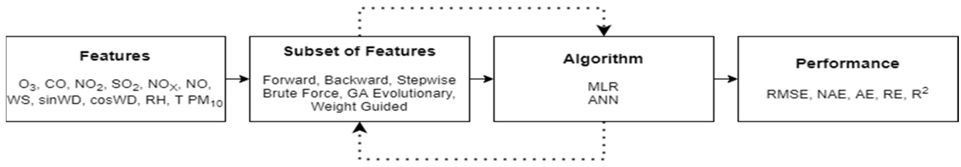
As shown in Figure 1, data acquisition, exploration, cleaning, transform and partitioning the data set are part of the data preparation. As for the feature selection, the partition data will be implemented in six wrapper methods, which are forward selection, backward elimination, stepwise, brute-force, weight-guided and genetic algorithm evolution. The significant variables obtained according to each method later will be used to develop predictive models, and MLR and ANN and will be evaluated using performance indicators. The performance of each model in MLR and ANN later will be compared and ranked according to its performance. The best model for each day of MLR and ANN will be compared again between the predictive analytics model. The best model obtained will be used to predict the concentration of PM₁₀ for the next day.

This section consists of data acquisition, data exploration, data cleaning, data transform and partitioning the dataset. The data acquisition will explain the information of data and parameters included in this study. Second, this study will conduct descriptive analysis in data exploration. Third, data cleaning will explain the technique involved in imputing the data. Next, data transform will explain the transformation on the data before being analyzed. Lastly, data partitioning will explain the partition of the dataset.

As for the data acquisition, this research used ten years of daily data on pollutant concentrations from two stations obtained from the Department of Environment Malaysia (DOE) from 2009 until 2018. The stations included in this study are Klang station located at Sekolah Menengah Perempuan Raja Zarina, Klang and Shah Alam station located at Sekolah Kebangsaan TTDI Jaya, Shah Alam. These two stations were selected because they are surrounded by major roads that experience heavy traffic, particularly during the morning rush hour.

Based on the Exploratory Data Analysis (EDA), this analysis measured the central tendency, dispersion, skewness and graphical representation. This study measured the central tendency of the data by estimating the mean, mode and median. This study also computed the variance, standard deviation and range in measuring the dispersion. Moreover, this research evaluated the skewness to check for the probability distribution of the data.

In this study, linear interpolation and the series mean are used to impute the missing values in the data as suggested by others [13]. Linear interpolation is an interpolation method for single-dimensional data. This method estimates the data point value needed to be interpolated based on the two data points adjacent to that point in the single-dimensional data sequence. Equation (1) shows the formula and graph of linear interpolation. While the series means method was used to impute all missing values with the mean value of the data. Therefore, the data was imputed using linear interpolation first, and the rest was imputed using the series mean.

$$y=y_i+\frac{\left(x-x_i\right)\left(y_2-y_1\right)}{\left(x_2-x_1\right)}$$

(1)

Based on the data retrieved, the readings of each parameter were recorded hourly. As this study predicts the PM₁₀ concentration by day, the data is transformed into a daily format. This study used the average PM₁₀ concentration of hourly data as the daily data. Next, the wind direction parameters in this study were split into two variables following [14]. The variables were the sinusoidal (sinWD) and the cosinusoidal (cosWD).

Before developing the model, the original dataset was divided into three datasets for training, validation and verification so that there would be new data to assess the model. The dataset collected for this study was divided chronologically into 80% for training data (2009–2016) and 20% for validation data (2016–2017). The training data was for estimating the predictive method parameters, while the validation data is for analyzing the accuracy. The proposed model was verified using the new dataset for 2018.

2.1. Feature Selection

Feature selection is the process of minimizing the number of input variables when building a predictive model [15]. In this research, the wrapper method was used to develop air pollution prediction modelling consisting forward selection, backward selection, stepwise selection, brute-force feature selection, Genetic Algorithm (GA) evolutionary and weight-guided.

Forward selection is a type of stepwise regression that begins with a null model. The approach initiates with no variables in the model and step by step adds variables to the model until no variable not included in the model can make a significant contribution to the model’s conclusion. The variable with the highest test statistic that is more than the cut-off value or the lowest p-value with less than the cut-off value is chosen and added to the model.

Backward elimination is the most basic approach to variable selection. This technique begins with a complete model that includes all of the variables in the model. Variables are subsequently removed from the whole model one by one until all remaining variables are sure to have a meaningful impact on the result. The variable with the lowest test statistic or the highest p-value more than the cut-off value is removed from the model. This procedure is repeated until every remaining variable is statistically significant at the cut-off value.

The stepwise selection method is the mixture of forward selection and backward elimination procedures that allow one to go in both directions while adding and eliminating variables at various stages. Forward selection and backward elimination can be applied to begin the process. If stepwise selection begins with forward selection, variables are added to the model one at a time according to the statistical significance. After each step, the model is analyzed. Any variable that is not significant will be removed from the model. The process repeats until every variable in the model is statistically significant.

If stepwise selection begins with backward elimination, the variables are removed from the full model based on statistical significance and then re-added if they show statistical significance afterward. Brute-force is a straightforward approach to solving a problem. It involves iterating through all possible features until the best feature selection is found. Brute-force feature selection tries every potential combination of the variables and provides the highest performing subset. The best subset is chosen by maximizing a defined performance metric in the presence of an arbitrary regressor or classifier. The algorithm will choose each combination and compute its score before selecting the optimal combination based on its score.

For this study, the number of possible subsets is calculated using the best subset regression formula, 2 p, where p equals 11 (the number of predictors). As a result, this method will generate 2048 subsets. Essentially, this method starts with the generation of possible subsets, beginning with one variable, two variables, three variables and so on until eleven predictors are generated. Each subset will have its own regression equation, which will be evaluated using the adjusted R square (${\overline{R}}^2$). The reason for using ${\overline{R}}^2$ rather than R² to compare the performance of subsets is that ${\overline{R}}^2$ values are often artificially inflated as more variables are chosen. The formula for ${\overline{R}}^2$ is stated below:

$${\overline{R}}^2=1-\left(1-R^2\right)\frac{n-1}{n-p-1}$$

(2)

where p is the number of predictors and n is the number of samples. The best subset, which contains the most significant factors to predict PM₁₀ concentration, will be the subset with the highest $R^2$ value.

Next, GA evolution is a type of optimization technique that mimics the concepts of natural evolution. There are three basic concepts in this process, which are selection, crossover and mutation. The first step of an evolutionary algorithm is an initialization phase where it creates a population of air pollution models, each with their unique set of chromosomes. The chromosomes are binary strings; 1 means the feature is included, and 0 means the feature is excluded. The models for the starting population are randomly generated.

A good rule of thumb is to use between 5% and 30% of the total number of features as the population size [16]. For the second step, each model in the population will have their fitness calculated. Models with better fitness have a higher chance of being chosen for recombination. After calculating the fitness value, the third step is that the models will be selected randomly using the roulette wheel method and selected according to their fitness level. The number of selected models is half of the population size.

After selecting the models, the fourth step is the crossover, in which the selected models are recombined to create a new population. In this step, two models will be chosen at random and their features will be combined to produce offspring for the new population until the new population is the same size as the old one. In the crossover, offspring that are genetically identical to their parents may be produced, resulting in a low-diversity new generation. Therefore, in step five, the mutation is done by changing the value of some features in the offspring at random. Lastly, the process is looped to step two until a stopping criterion is met and the best feature selection is obtained.

Finally, the wrapper method used weight-guided via correlation. Equation (3) is the formula of the correlation. A weight is given to the variables, and the highest weight of the variable is considered.

$$r=\frac{n(\sum xy-\left(\sum x\right)\left(\sum y\right))}{\sqrt{[n\sum x^2-{\left(\sum x\right)}^2]}[n\sum x^2-{\left(\sum x\right)}^2]}$$

(3)

2.2. Model Development and Model Evaluation

In this model development, the process of developing MLR and ANN models is explained to conduct predictive modelling. Figure 2 shows the process of the wrapper method in developing a predictive model.

There are four steps in developing a multiple linear regression (MLR) model. First, the development of the MLR model will be based on 80% of the data. Second, the assumption of the MLR models is checked using certain methods and tests, such as histograms and scatter plots. Next, the model is validated based on the performance indicator value using 20% of the data. Finally, the best model of MLR is obtained. The expected MLR models are as shown in Equation (4). The past PM₁₀ daily average concentration was used to predict the next day’s PM₁₀ concentration.

PM_10,D+1 = β₀ + β₁PM_10,D + β₂CO_D + β₃NO_2,D + β₄NO_x,D + β₅NO_D + β₆SO_2,D +
β₇RH_D + β₈T_D + β₉WS_D + β₁₀cosWD_D + β₁₁sinWD_D

(4)

where

PM_10,D+1 = Next day prediction of PM₁₀ concentration.

PM_10,D = Particulate matter (µg/m³).

CO_D = Carbon monoxides (ppm).

NO_2,D = Nitrogen dioxide (ppm).

NO_x,D = Nitrogen oxide (ppm).

NO_D = Nitric oxide (ppm).

SO_2,D = Sulfur dioxide (ppm).

RH_D = Relative humidity (%).

T_D = Temperature (°C).

WS_D = Wind speed (km/h).

cosWD_D = Cosine Wind direction (units).

sinWD_D = Sine Wind direction (units).

β₀ = regression constant.

β_1, …, β₁₁ = regression coefficient for each predictors used.

A feed forward backpropagation neural network (FFBP) was used in this study. The structure of FFBP was composed of three layers of neurons called the input, hidden and output layers. The first layer of neurons consisted of an input layer, representing independent variables. The input layer contained 12 independent variables—namely, O₃, CO, NO₂, SO₂, NO, sinWD, cosWD, NOx, PM₁₀, T, WS and RH. The second layer was the hidden layer, which is responsible for processing the input weight from the input layer and transferring it to the output layer. The third layer was the output layer, which represents the PM_10,D+1 concentrations.

The maximum error used as a criterion for stopping was set at 0.05. In this study, the training process was set to 10,000 iterations or until the maximum error was reached, as suggested by [17]. As a network training function, Levenberg–Marquardt optimization was used to update weight and bias values. As sigmoid units are easier to train than other activation functions, [18] proposed using them. In this case, the layer size was 2 number of attributes + number of classes)/2 + 1 = 8 hidden nodes, as recommended by [19]. This study fitted models with varying learning rate lr (0.01) values, which [20] proposed for the study of air pollution datasets.

Furthermore, [21] stated that changing the momentum rate and learning rate from 0.05 to 1 had no effect on the training and prediction networks’ errors. Performance indicators in this research are used to identify the best method to predict the concentration of PM_10,D+1. The Root Mean Square Error (RMSE), Normalized Absolute Error (NAE), Absolute Error (AE) and Relative Error (RE) are the error measures used to determine the error of the model, while the Coefficient of Determination (R²) is the accuracy measure used to determine the accuracy of the model outcome.

Regarding the model deployment, the dataset from 2009 until 2017 was used to produce prediction models. The prediction models were later deployed on the 2018 dataset. However, there were extreme outliers in ozone concentration for the 2018 dataset for the Klang station. Based on the 2009 until 2017 dataset, the maximum ozone concentration value was 0.056 ppb. Some of the ozone concentration in the 2018 dataset exceeded 0.7 ppb. This situation may happen due to technical errors. Therefore, a total of 29 data were removed before deployment.

3. Results and Discussion

3.1. Descriptive Analysis

Table 1. Descriptive statistics for Klang and Shah Alam.

		Mean	Median	Standard Deviation	Skewness	Minimum	Maximum
	WS (km/h)	5.38	5.80	2.03	4.89	0.47	52.03
	WD (°)	176.78	168.83	46.05	0.579	42.17	318.17
	T (°C)	28.62	28.60	1.52	−0.12	22.56	33.12
K	RH (%)	69.74	69.62	7.07	0.01	46.46	94.11
L	NOX (ppm)	0.037	0.035	0.029	25.60	<0.01	1.14
A	NO (ppm)	0.016	0.014	0.028	31.6	<0.01	1.15
N	SO2 (ppm)	0.004	0.004	0.002	2.25	<0.01	0.03
G	NO2 (ppm)	0.02106	0.021	0.007	0.28	0.001	0.05
	O3 (ppm)	0.019	0.018	0.007	0.78	<0.01	0.06
	CO (ppm)	1.029	0.967	0.412	2.38	0.15	6.21
	${\mathrm{PM}}_{10}(\mathsf{\mu }\mathrm{g}/{\mathrm{m}}^3$)	62.75	56.16	32.52	4.62	17.18	551.54
	WS (km/h)	4.828	4.775	1.908	0.198	0.314	16.529
S	WD (°)	157.15	153.71	52.76	0.50	9.75	337.17
H	T (°C)	28.10	28.09	1.32	0.02	23.31	33.29
A	RH (%)	77.35	77.46	6.11	−0.05	54	94.63
H	NOX (ppm)	0.04	0.04	0.02	0.48	0.004	0.12
	NO (ppm)	0.02	0.02	0.01	1.11	<0.001	0.09
A	SO2 (ppm)	0.003	0.003	0.002	1.74	<0.001	0.02
L	NO2 (ppm)	0.02	0.02	0.01	0.45	0.002	0.06
A	O3 (ppm)	0.02	0.02	0.01	0.86	<0.001	0.08
M	CO (ppm)	0.76	0.73	0.30	1.18	0.09	3.69
	${\mathrm{PM}}_{10}(\mathsf{\mu }\mathrm{g}/{\mathrm{m}}^3$)	50.91	45.33	34.86	17.11	11.92	1332.81

is the descriptive statistics of each parameter in Klang and Shah Alam, Selangor. Based on the table, the maximum concentration of PM₁₀ was 551.542 µg/m³ (Klang) and 1332.814 µg/m³ (Shah Alam). The high concentration was taken on 25 of June 2013 for Klang, while Shah Alam happened during April 2017. Next, the skewness value of PM₁₀ is 4.62 (Klang) and 17.11 (Shah Alam). Since the value is more than 1, the data of PM₁₀ are highly skewed to the right. This may be due to the presence of extreme outliers in this data.

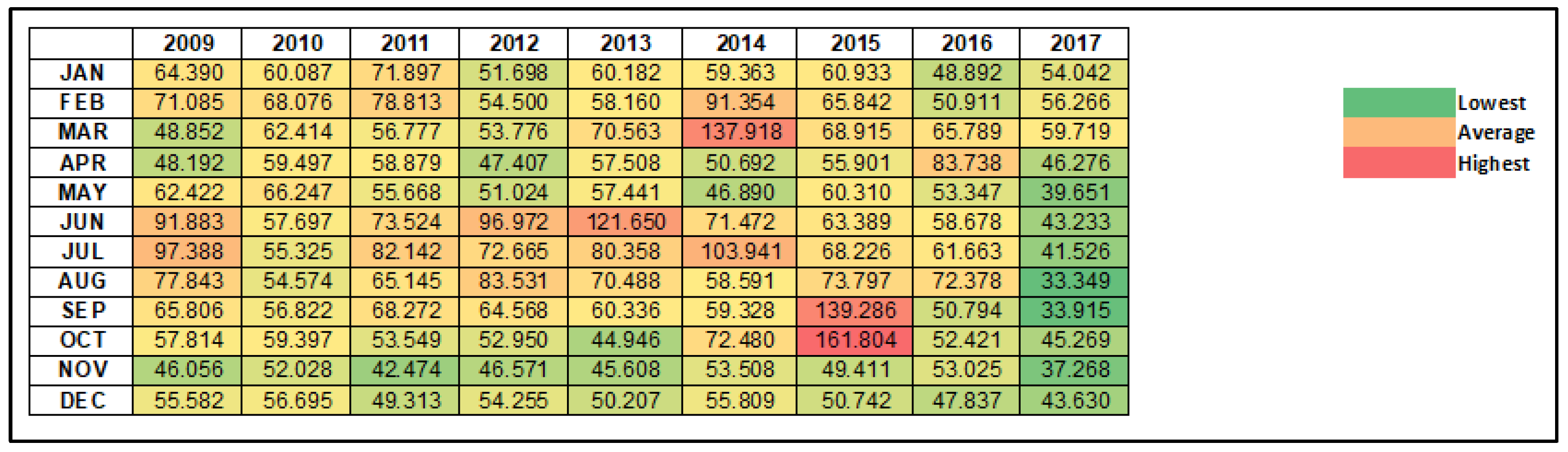
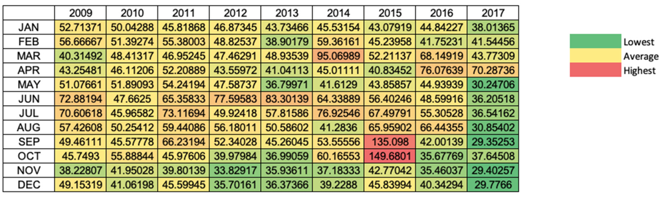
Figure 3 and Figure 4 below are heatmaps of the average PM₁₀ concentrations according to the month and year for Klang and Shah Alam. The greenish parts have the lowest average concentration, and the reddish parts have the highest average concentration. Based on both Figures, it is indicated that October 2015 had the highest average concentration compared to the others. Moreover, the concentration of PM₁₀ in September 2015 was the second-highest concentration. Referring to haze incidents in Malaysia, this supports the outline of the heatmap as there was a hazing incident in 2015 in August and September due to massive land and forest fires in Indonesia [22]. The high PM₁₀ concentration in October 2015 may be due to the backlash of this incident.

In March 2014, there was a high concentration of PM₁₀ in both locations where Klang was slightly higher than Shah Alam. It is also proved by the chronology of haze incidents in Malaysia as haze incidents happened between February and March 2014. This incident occurred due to forest and peatland fires. High PM₁₀ concentration incidents were also detected in June 2013 from both locations. However, Klang had a higher concentration value compared to Shah Alam. This incident may be due to haze incidents that happened from 15 to 27 June 2013 [22]. In addition, both Figures show a low average of PM₁₀ concentration starting from May until December 2017. This situation may be due to zero cases of haze incidents happening in 2017.

In conclusion, the heatmaps of both locations align with the haze chronology in Malaysia. The heatmaps also makes it easier to observe the condition of air pollution in Malaysia.

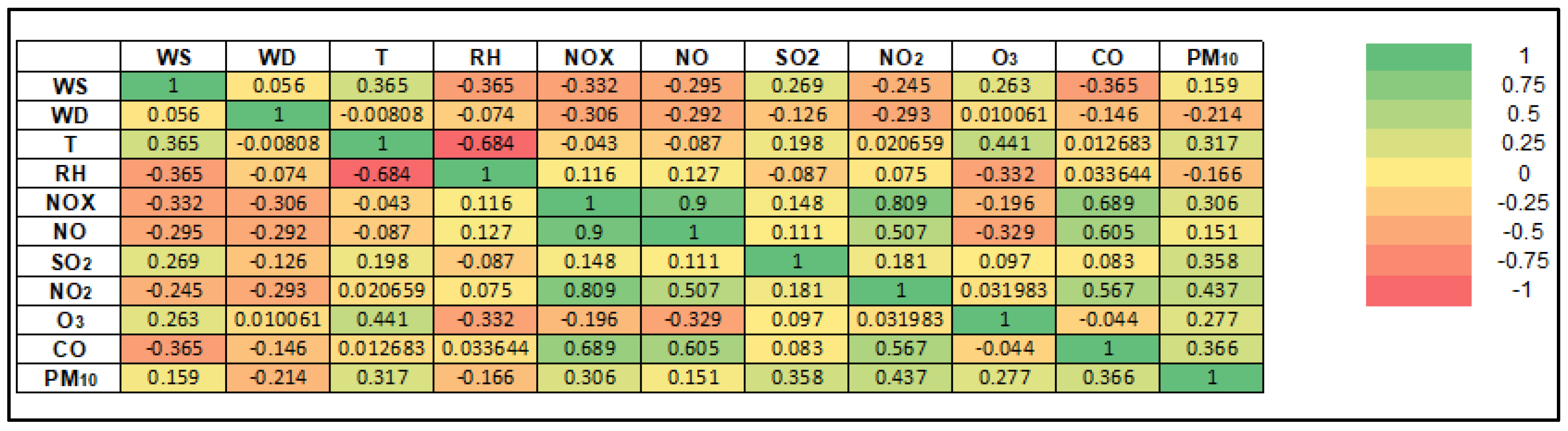
3.2. Correlation of PM₁₀ Concentration with Other Parameters

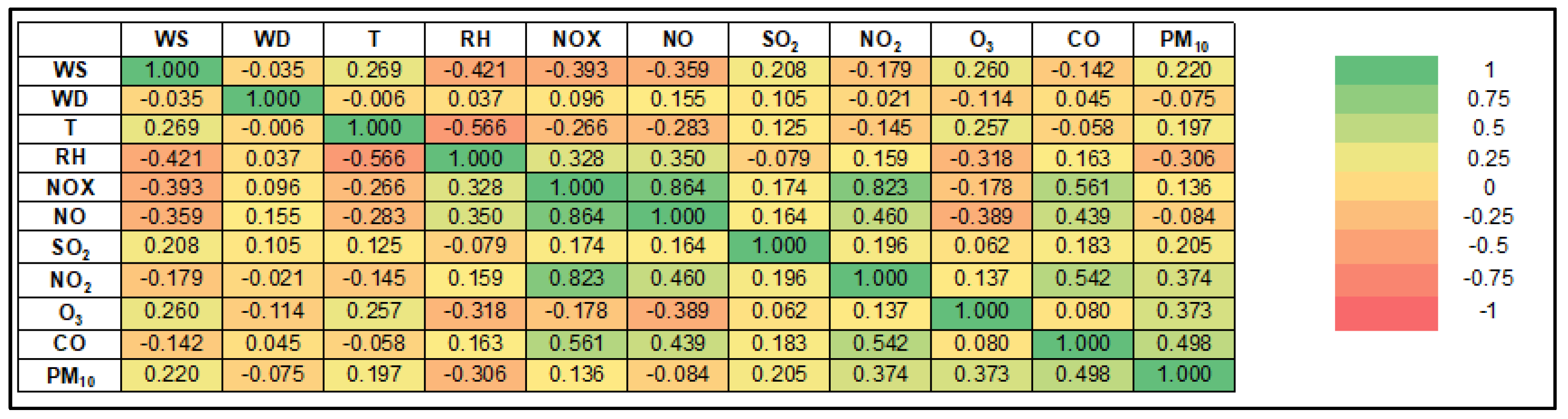
Figure 5 and Figure 6 show the heatmap of the Spearman’s rank correlation coefficient (r) of the PM₁₀ concentration with other parameters in Klang and Shah Alam, respectively. Figure 5 shows that all of the parameters have positive correlation with PM₁₀ except for WD, RH and NO in Klang. It also indicates all of the parameters have moderate-to-very-weak correlations with the PM₁₀ for Klang. CO has the highest correlation PM₁₀ concentration with a positive moderate correlation (r = 0.498), while WD has the lowest correlation with a negative very weak correlation (r = −0.075).

Figure 6 shows that all of the parameters have a positive correlation with PM₁₀ except for WD and RH in Shah Alam. All of the parameters have moderate, weak and very weak correlations with the PM₁₀ concentration. It also indicates that NO₂ has the highest correlation with PM₁₀ concentration with a positive moderate correlation (r = 0.437), while WD has the lowest correlation with PM₁₀ concentration with a positive very weak correlation (r = 0.151).

3.3. Performance Model and Feature Selection

Performance measures for this section used the validation dataset (20%).

Table 2. Performance models of MLR for Klang and Shah Alam for the validation.

Location	Method	RMSE	AE	RE	NAE	R2
Klang	Forward	14.224	10.292	17.97%	0.596	0.709
	Backward	14.186	10.447	18.17%	0.605	0.713
	Stepwise	14.224	10.292	17.97%	0.596	0.709
	Brute-Force	13.694	10.005	17.52%	0.596	0.707
	Weight-Guided	16.27	11.089	19.21%	0.658	0.591
	Evolution	14.367	10.701	18.84%	0.633	0.665
Shah Alam	Forward	15.176	10.932	23.99%	0.709	0.598
	Backward	15.23	11.346	24.77%	0.736	0.502
	Stepwise	15.176	10.932	23.99%	0.709	0.598
	Brute-Force	12.338	9.559	21.77%	0.662	0.632
	Weight-Guided	13.417	10.371	25.92%	0.722	0.596
	Evolution	14.530	11.411	26.84%	0.782	0.531

shows that the performance of all MLR model was compared to find the best model for next day prediction. Based on

Table 3. Ranking performance models of MLR for Klang and Shah Alam.

Location	Method	RMSE	AE	RE	NAE	R2	Total Rank
Klang	Forward	3	2	3	1	2	11
	Backward	2	3	4	2	1	12
	Stepwise	3	2	2	1	2	10
	Brute-Force	1	1	1	1	3	7
	Weight-Guided	5	5	6	4	5	25
	Evolution	4	4	5	3	4	20
Shah Alam	Forward	4	3	2	2	2	13
	Backward	5	4	3	4	5	21
	Stepwise	4	3	2	2	2	13
	Brute-Force	1	1	1	1	1	5
	Weight-Guided	2	2	4	3	3	14
	Evolution	3	5	5	5	4	22

, for Klang, brute-force has the lowest value of RMSE, AE, RE and NAE. The backward method has the highest R² value compared to others.

Therefore, it is shown that brute-force is the best model for Klang as it had the lowest value of error and the lowest total rank with WS, RH, SO₂, O₃ and PM₁₀ as the parameters selected to predict the next day’s PM₁₀ concentration. Furthermore, the performance for all models in predicting PM₁₀ in Shah Alam also shows that brute-force had the lowest error measures for RMSE, AE, RE and NAE and the highest accuracy for R². Therefore, brute-force is the best model with T, RH, SO₂, NO₂, sinWD, NO and PM₁₀ as the parameters selected to predict the PM_10,D+1.

Referring to

Table 4. Selected features of MLR for Klang and Shah Alam.

Location	Method	WS	T	RH	SO2	NO2	O3	CO	Sin WD	Cos WD	NOX	NO	PM10
Klang	Forward		/	/									/
	Backward	/		/	/	/	/	/		/	/		/
	Stepwise			/									/
	Brute-Force			/	/		/						/
	Weight-Guided												/
	Evolution	/		/				/		/			/
Shah Alam	Forward	/		/				/		/			/
	Backward	/			/								/
	Stepwise		/		/		/	/	/	/	/	/	/
	Brute-Force	/			/								/
	Weight-Guided		/	/	/	/			/			/	/
	Evolution												/

, the ticked table means that the parameter is selected in that model. For the best model PM_10,D+1 for Klang (MLR-Brute-Force), RH, SO₂, NO₂, O₃ and PM₁₀ were analyzed to predict the next day for Klang. For the best model PM_10,D+1 for Shah Alam (MLR-Brute -Force), T, RH, SO₂, NO₂, sinWD, NO and PM₁₀ are the parameters selected to predict the next day for Shah Alam.

Based on

Table 5. Performance models of ANN for Klang and Shah Alam for validation.

Location	Method	RMSE	AE	RE	NAE	R2
Klang	Forward	15.517	11.067	19.57%	0.588	0.701
	Backward	15.085	10.272	17.06%	0.574	0.742
	Stepwise	15.517	11.067	19.57%	0.588	0.701
	Brute-Force	14.139	10.282	16.90%	0.605	0.701
	Weight-Guided	17,288	11.779	18.64%	0.699	0.581
	Evolution	14.228	10.335	17.92%	0.563	0.732
Shah Alam	Forward	13.448	9.317	18.93%	0.594	0.715
	Backward	14.071	9.595	20.19%	0.647	0.596
	Stepwise	12.966	9.505	22.30%	0.65	0.691
	Brute-Force	12.252	9.138	20.75%	0.614	0.687
	Weight-Guided	12.463	8.840	18.72%	0.615	0.615
	Evolution	14.003	10.005	21.83%	0.645	0.657

, the performances of all ANN models for next-day prediction in Klang and Shah Alam were compared to determine the best model. For Klang, brute-force had the lowest value of RMSE and RE, and backward had the lowest value AE and highest R² value compared to the others. Evolution had the lowest value of NAE. However, backward is the best model for Klang station as it had the lowest total rank compared to the others with T, RH, SO₂, NO₂, O₃, sinWD, cosWD, NO_x, NO and PM₁₀ as the parameters selected to predict the PM_10,D+1.

Next, the performance for all ANN models in predicting PM_10,D+1 in Shah Alam shows that brute-force had the lowest value for RMSE, weight-guided had the lowest value for AE and RE, and forward had the lowest value for NAE and the highest value for R². However, forward is the best model in predicting PM_10,D+1 since it hd the lowest total rank with WS, NO_X and PM₁₀ as the parameters selected to predict the PM_10,D+1 as shown in

Table 6. Ranking the performance models of ANN for Klang and Shah Alam.

Location	Method	RMSE	AE	RE	NAE	R2	Total Rank
Klang	Forward	4	4	4	3	3	18
	Backward	3	1	2	2	1	9
	Stepwise	4	4	4	3	3	18
	Brute-Force	1	2	1	4	3	11
	Weight-Guided	5	5	5	5	4	24
	Evolution	2	3	3	1	2	11
Shah Alam	Forward	4	3	2	1	1	11
	Backward	6	5	3	5	6	25
	Stepwise	3	4	6	6	2	21
	Brute-Force	1	2	4	2	3	12
	Weight-Guided	2	1	1	3	5	12
	Evolution	5	6	5	4	4	24

.

Referring to

Table 7. Selected features of ANN for Klang and Shah Alam.

Location	Method	WS	T	RH	SO2	NO2	O3	CO	Sin WD	Cos WD	NOX	NO	PM10
Shah Alam	Forward	/									/		/
	Backward				/	/	/		/	/		/	/
	Stepwise	/
	Brute-Force	/	/	/		/	/				/		/
	Weight-Guided												/
Klang	Forward								/		/		/
	Backward		/	/	/	/	/		/	/	/	/	/
	Stepwise								/		/		/
	Brute-Force	/		/	/						/	/	/
	Weight-Guided												/
	Evolution			/		/	/	/		/	/		/

, the ticked (/) table means that the parameter is selected in that model. For the best model PM_10,D+1 for Klang (ANN-Backward), RH, SO₂, NO₂, O₃, PM₁₀, sinWD, cosWD, NO_X and NO were analyzed to predict the next day. For the best model PM_10,D+1 for Shah Alam (ANN-Forward), WS, NO_{X and} PM₁₀ are the parameters selected to predict the next day for Shah Alam using ANN.

As a conclusion, brute-force is the best feature selection to predict the next day’s PM₁₀ concentration in Klang and Shah Alam by using MLR, and the models fulfil the assumptions of MLR. The backward for Klang and forward for Shah Alam are the best feature selections for predicting the next day’s PM₁₀ concentration using the ANN model.

3.4. The Best Model

The best model to predict the PM_10,D+1 for each station was obtained by comparing the performance of models between MLR and ANN. For the overall performance, each predicted day shows that the ANN model had the best performance compared to the MLR model for both Klang and Shah Alam station. This result is supported with

Table 8. Performance ranking of the best model.

Station	Model	Method	RMSE	AE	RE	NAE	R2	Total
Klang	MLR	Brute-Force	1	1	2	2	2	8
	ANN	Backward	2	2	1	1	1	7
Shah Alam	MLR	Brute-Force	1	2	2	2	2	9
	ANN	Forward	2	1	1	1	1	6

as the ANN model for each predicted day for both stations shows the lowest total score. In Klang, ANN with backward elimination is the best model selected, while for Shah Alam, ANN with forward selection is the best model.

Furthermore, Table 9 summarizes the comparison results with other research. This indicates that the results in this study are similar to those in other studies. Regression is involved with linear dependencies, whereas neural networks are involved with nonlinearities. As a result, if the data contains nonlinear dependencies, neural networks should outperform regression.

According to studies [23,24,25], the ANN method predicts the dependent variable more accurately than MLR. Although ANN is regarded as a powerful technique for non-linear models [26], some researchers have used and reported on this linear model better than the regression model [27,28,29]. This showed that our ANN model can be used to predict PM₁₀ concentrations since it improved the performance of the model.

Table 9. Performance indicators results gained from other research.

Authors	Method	Result
[30]	MLR	${\mathrm{R}}^2$ = 0.347–0.614
[31]	MLR	RMSE = 126.728–164.978 NAE = 0.325–0.429 PA = 0.359–0.668
[32]	MLR	${\mathrm{R}}^2$ = 0.3239
[33]	MLR	${\mathrm{R}}^2$ = 0.586–0.715
This Study	ANN-Forward ANN-Backward MLR-Brute-Force	R2 = 0.63–0.74 RMSE = 12.33–15.08

Table 9. Performance indicators results gained from other research.

Authors	Method	Result
[30]	MLR	${\mathrm{R}}^2$ = 0.347–0.614
[31]	MLR	RMSE = 126.728–164.978 NAE = 0.325–0.429 PA = 0.359–0.668
[32]	MLR	${\mathrm{R}}^2$ = 0.3239
[33]	MLR	${\mathrm{R}}^2$ = 0.586–0.715
This Study	ANN-Forward ANN-Backward MLR-Brute-Force	R2 = 0.63–0.74 RMSE = 12.33–15.08

3.5. Model Verification

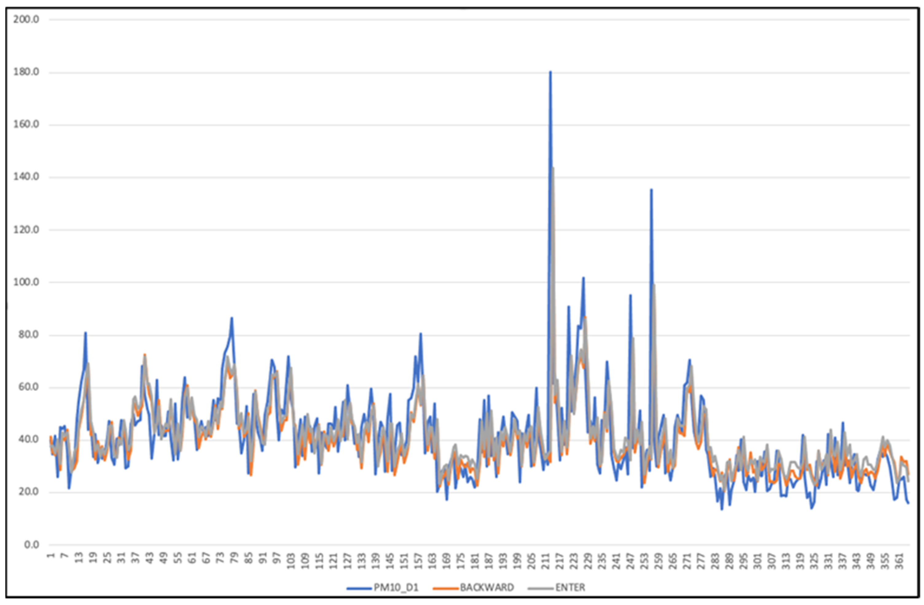
For the model verification, the dataset from 2009 until 2017 was used to develop prediction models. The proposed prediction models were used to predict the PM₁₀ concentration using the 2018 dataset [30,31,32,33,34,35]. Figure 7 and Figure 8 below show line charts of the observed and predicted values of the PM₁₀ concentration in Shah Alam and Klang.

This predictive model used ANN with backward elimination using RH, SO₂, NO₂, O₃, PM₁₀, sinWD, cosWD, NO_X and NO as a parameters in Klang. For the best model PM_10,D+1 for Shah Alam (ANN-Forward), WS, NO_X and PM₁₀ are the parameters selected to predict the next day for Shah Alam using ANN.

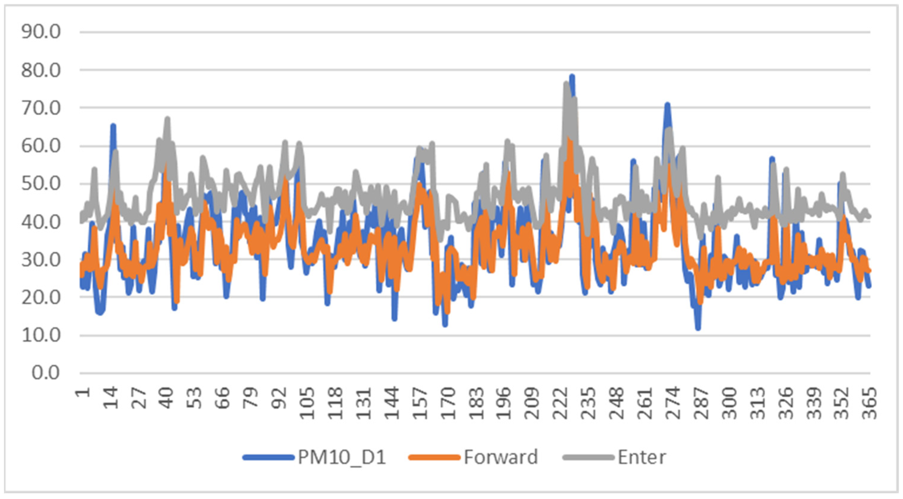
Figure 7 shows the comparison of the line chart between the observed and predicted value for PM_10,D+1 for model ANN-forward selection and predicted ANN using all variables. Referring to the line chart, it shows that, on average, the observed and predicted values have a slight gap. Most of the prediction values exceed the observed value; however, in some cases, the observed value exceeds the prediction value. Furthermore, the enter method has a large gap since, in 2018, there was a slight increase in the value of ozone, causing the prediction using all parameters to be higher than the observed value. Therefore, it shows that the predicted values of the PM₁₀ concentration were not notably affected by the ozone concentration.

Overall, the values of RMSE and AE of this model are 20.728 and 15.69, respectively. Hence, this model can be used for unseen data since there is no huge difference between the observed and predicted values. Figure 8 shows the comparison of the line chart between the observed and predicted values for PM_10,D+1 for the model ANN-forward selection and predicted ANN using all variables. Referring to the line chart, it shows that, on average, the observed and predicted values have a minimum gap between each other with the value of RMSE at 10.004 and value of AE at 7.982. Most of the prediction values exceed the observed value, and in only a few cases does the observed value exceed the prediction value. Hence, this model can be used for unseen data since there is no great difference between the observed and predicted values.s

The prediction error in Klang is higher than in Shah Alam because the industrial area of Klang suffers from severe haze, while Shah Alam is only a residential area. Furthermore, if all variables based on previous studies are selected to predict PM₁₀ concentrations for the next day, it will take more time to determine the best model and reduce the maintenance data cost for the future.

4. Conclusions

In this study, the wrapper methods of six different feature selections were analyzed and compared to determine the best feature selection method. The methods included were forward, backward, stepwise, brute-force, weight-guided and GA evolution. These methods were analyzed together with the predictive analytics methods MLR and ANN. The performance of the models determined the best model to predict the next day. This study found that the best feature selections were backward elimination, forward selection and brute-force in predicting the PM₁₀ concentration in Malaysia.

Based on the results, the best feature selection method to predict the PM_10,D+1 in Klang was the backward method with the parameters T, RH, SO₂, NO₂, O₃, PM₁₀, sinWD, cosWD, NOX and NO. For Shah Alam, the best feature selection method to predict PM_10,D+1 was the forward method with the parameters WS, NO_X and PM₁₀.

The prediction of the ANN model for PM_10,D+1 was deployed in the 2018 dataset. Based on the line chart in Figure 7 and Figure 8, the gaps between the observed and predicted lines show a minimum difference. The RMSE value in Klang for PM_10,D+1 was 20.728, while the AE value was 15.69. In addition, the line chart of observed and predicted of each predicted day in Shah Alam also shows a minimum gap between each line with the RMSE value for PM_10,D+1 of 10.004, while the AE value was 7.982. In conclusion, all of the predicted models in Klang and Shah Alam can be used for unseen data.

There are a few recommendations for improving the performance of air pollution modelling that can be suggested to other researchers. This study used the cross-sectional method, and for future research, we suggest using time series, since the time-series forecasting method is better at predicting extreme events compared to the cross-sectional method. Apart from the MLR and ANN models, a new approach can be implemented to the predicted modelling to forecast the concentration of PM₁₀ using machine-learning methods, such as long short-term memory (LSTM), gated recurrent units (GRU) and deep learning [36].

Other methods, aside from wrapper methods, can be applied to conduct feature selection for air pollution modelling, such as the filter method, embedded method and hybrid method. Hence, various approaches to predicted modelling and feature selection methods for air pollution modelling will be beneficial as they will produce better results. In addition, predictions for other particulate matter, such as PM_2.5, should be made since the DOE began to include PM_2.5 in calculating the API from 2018. In addition, PM_2.5 is more dangerous since the size of the particles is smaller compared to PM₁₀. Therefore, predicting PM_2.5 may help to improve the performance of air pollution modelling. Lastly, this output can be used by the authorities as it will be helpful to reduce the impact of air pollutants.

For example, the DOE’s prediction of air pollutants can be used for early alertness to help in performing the relevant procedures. Hopefully, this recommendation will help improve air pollution modelling and help the authorities to pay early attention to the air pollutants in Malaysia. The limitation of this research is that the model can only be used when the sources and conditions of the characteristics of PM₁₀ remain the same. Therefore, it may not be suitable for the other locations. For instance, if there is a sudden forest fire or storm in a selected area, this would affect the PM₁₀ concentration.