Implications of the Emergence of Autonomous Vehicles and Shared Autonomous Vehicles: A Budapest Perspective

Abstract

The introduction of autonomous vehicles (AVs) and shared autonomous vehicles (SAVs) is projected to enhance network performance and accessibility. The future share distribution of AV and SAV is not yet apparent, nor is which of these two future transport modes will become dominant. Therefore, this research deploys a simulation-based dynamic traffic assignment using Visum software to investigate the impact of varying the share distribution of AVs and SAVs on Budapest’s network performance and consumer surplus in three projected future traffic scenarios for the years 2030 and 2050 compared to the Base scenario for 2020. The three future scenarios are presented and characterized by different penetration rates of AVs and SAVs to reflect the uncertainty in the market share of these future cars as follows: Mix-Traffic scenario for 2030, and AV-Focused and SAV-Focused scenarios for 2050. The results revealed that the emergence of AVs and SAVs would improve the overall network performance, and better performance was observed with increasing the share distribution of SAVs. Similarly, the consumer surplus increased in all future scenarios, especially with increasing the share distribution of AVs. Consequently, the advent of AVs and SAVs will improve traffic performance and increase consumer surplus, benefiting road users and authorities.

1. Introduction

The vehicle industry, policymakers, and academia pay attention to rapid global research and innovation connected to autonomous vehicles (AVs), shared autonomous vehicles (SAVs) [1], and their projected appearance on roadways [2,3]. Due to their benefits, AVs and SAVs are projected to dominate automobile markets [4]. Additionally, several laws relating to the deployment of AVs and SAVs have been effectively implemented in many nations and areas [5]. Thanks to the evolution of information and communication technology and mobile solutions, ride-sharing services have become more popular in several cities since the 2010s [6]. Such services provide users with cheaper and more versatile commuting options [7]. Moreover, they are associated with lower vehicle ownership [8] and greenhouse gas emissions [9]. Because of their rising popularity and cheaper travel costs compared to privately owned vehicles, shared mobility services are predicted to prosper in the future and provide the first appearance of self-driving cars in the frame of SAVs [10]. This is especially true with electric SAVs, which are expected to be widely adopted and provide a more viable society [11,12]. Furthermore, SAVs are expected to emerge as a demand-responsive service [13].

The benefits of automated vehicles are predicted to be significant, notably in terms of traffic safety, energy usage, and accessibility [14]. In terms of traffic, AVs and SAVs will assist in relieving congestion by lowering the number of accidents due to human mistakes, shortening headways, and optimizing the use of intersections [15]. Furthermore, as these vehicles do not require human interaction to finish the journey, users of AVs and SAVs may better use their travel time by doing other activities like studying or relaxing instead of monitoring the road or navigating [16]. Nevertheless, AVs and SAVs are anticipated to boost the number and mileage of the trips driven by providing new groups of users, who were before unable to travel by cars owing to various considerations such as age or disability, with more flexibility in commuting, resulting in increased traffic [14]. As a result, the impacts of AVs and SAVs on road congestion are yet unclear [17], and they may exacerbate existing traffic issues [18]. Furthermore, the research studies on self-driving vehicles’ influence on various areas of mobility, such as traffic performance, travel behavior, and social welfare, are rapidly growing [19]. This study introduces AVs and SAVs together utilizing the simulation-based dynamic traffic assignment (SBA) using Visum software for the city of Budapest to answer the following research questions:

• What effects do AV and SAV deployments in Budapest have on the following traffic performance parameters (TPP): average and maximum queue lengths, delays, volume, density, utilization (scaled density), velocity, and vehicle kilometers traveled (VKT)? What are the implications of implementing AVs and SAVs concerning consumer surplus (CS)?
• How do varying the share distribution of AVs and SAVs affect traffic performance and CS?

To that end, we compare the impact of deployment of AVs and SAVs on Budapest’s network traffic performance and CS in alternative future traffic scenarios to the Base scenario, which describes the current traffic situation in Budapest based on projected travel demand for the year 2020. Three possible future traffic scenarios are presented, each characterized by varying AV and SAV replacement rates of conventional vehicles (CC), to reflect the uncertainty in self-driving vehicles’ emergence possibilities based on projected travel demand for the years 2030 and 2050. The travel demand of the developed scenarios was obtained from The Centre for Budapest Transport (BKK) projections for the respective years. The Mix-Traffic scenario for 2030 combined CC, AVs, and SAVs as all coexisting on the network. Two more alternative future scenarios are based only on the inclusion of AVs and SAVs in the network and were set for the year 2050, with the AV-Focused scenario implying a strong reliance on commuting by privately owned AVs, and the SAV-Focused scenario implying a high reliance on using the fleet of SAV.

As this research investigates the implications of introducing new mobility solutions and alternative vehicles, including conventional, electrical, and automated vehicles, along with introducing a shared mobility system, it is related to the following concepts, which amount to relevant current and future challenges: sustainable mobility at the urban level and the possibility of preparing national, local, and regional transport plans [20,21]. Sustainable mobility as a service (MaaS) includes managerial components “sharing mobility” and material components “autonomous mobility” [22]. While the evolution of mobility concerns people’s future mobility patterns [23].

The rest of the work is presented as follows: an explanation of the Budapest network model, as well as the SBA framework for AVs and SAVs, which was built using the Visum software and utilized in this study in Section 2. Then Section 3 delves deeper into the development of future traffic scenarios. After presenting and discussing the results in Section 4, the research’s conclusions are emphasized Section 5.

2. Research Methodology

This section goes through the dynamic traffic assignment framework while providing an outline of the Visum software developed by Planung Transport Verkehr (PTV) and the Budapest transport model, Egységes Forgalmi Modell (EFM), adopted in this research; and provides a comprehensive overview of AV and SAV implementation methods.

2.1. PTV Visum and EFM Macroscopic Model

Budapest is Hungary’s capital, with a community of over 1.76 million people who live in a 525-square-kilometer space and more than 4.61 million travelers visiting annually [24]. PTV Visum software has been used to design Budapest’s transport network. Visum is a software for traffic macroscopic simulation, which can model various modes of transportation and simulate their traffic demands utilizing calculated Origin-Destination (O-D) matrices while keeping in view a specified road network. It lets users integrate network data from a wide variety of providers, like Open Street Map. Moreover, it is often utilized to design as well as evaluate transport networks, initiatives, and solutions, involving individual and collective traffic patterns. This is built on the well-known four-step modeling approach (viz., trip generation, trip distribution, mode choice, and route assignment). The Visum software was picked for this research to plan and examine the implications of different possibilities of emerging AVs and SAVs in future traffic situations. The key reasons for choosing it are: the essence of the evaluation, which is a macro-simulation that depends on different features of traffic flow, including density, velocity, volume, and delay; the provision of a fully prepared network model for Budapest in Visum titled the EFM Model, which contains relevant information like O-D matrices, free-flow velocity, and traffic volumes; and Visum can assign and evaluate new modes of transportation (i.e., AVs and SAVs).

BKK used Visum software to produce the EFM Model for the city of Budapest and the vicinity. It comprises over 30,000 links that symbolize mainly roads and rails, as well as their actual traffic characteristics like permitted velocity, permissible types of vehicles, and the number of lanes. Around 15,000 nodes indicate the beginning and ending of every link, as well as the network’s intersections. 1200 zones were defined as the origin and destination of the network’s trips. The model was created and calibrated with information from a critical examination of traffic situations in 2014 that took into account a list of factors, including population, motorization, and economic situations. The three aspects of macroscopic modeling are included in the EFM Model (i.e., demand model, network model, and impact model). Likewise, the model provides a prediction of travel demand for the years 2020, 2030, and 2050, taking into consideration demographic estimations, motorization projections, and the effects of economic growth; these anticipated travel demands were used during the modeling process of future traffic scenarios. The following traffic prediction Equation (1) was used in the model:

$$C_t=S/\left(1+\left(\frac{S-C_0}{C_0}\right).e^{\frac{-g_0·S·t}{\left(S-C_0\right)}}\right)$$

(1)

where $C_t$ is the motorization value throughout the given year, $S$ is the motorization concentration degree (saturation), $C_0$ is the base year’s motorization degree, $g_0$ is the growth rate, and $t$ is the number of years since the base year.

Moreover, the EFM model is calibrated and validated for every mode of transport (i.e., taxis, freight transport, bicycles, and public transport (PuT)) in a careful way to emulate an accurate depiction of the traffic situations of network components with a small error range, thus providing reasonable estimations. The O-D matrices were calibrated utilizing around 240 cross-sections spaced across the city, and the estimated tolerance was calculated using the Geoffrey E. Havers (GEH) formula. The calibration results revealed that the values of cross-sectional traffic are tolerable relative to the counted traffic values. Since this investigation utilized SBA rather than static equilibrium assignment, a supplementary calibration was conducted to validate that the model is applicable to dynamic traffic assignment. The GEH function has been used for the new calibration with the highest value of 5 as an appropriate tolerable limit, similar to the first calibration. The calibration results show that 86% of the measured sections have a GEH index less than 5, which is recommended as it shows a good match between the modeled traffic volumes and observed traffic volumes [25].

In conclusion, the EFM Model is expertly developed and depicts an accurate version of the Budapest transport network; it can be applied to design, create, and accurately predict transport modifications in Budapest and its vicinity.

For more information related to the EFM model and the Visum Software, see [26,27].

2.2. SBA Implementation for AVs

The automation degree and the provision of appropriate infrastructure are key attributes in incorporating AV and SAV driving behavior into the transport network. If a segment of the network supports Vehicle-to-Vehicle (V2V) and Vehicle-to-Infrastructure (V2I) connectivity, AVs and SAVs can interact with one another, enabling the automated cars to drive in a defined headway and even form platoons. In this paper, such network links are termed “S/AV-ready”. The following two sub-sections cover the AV modeling approach and the parameters of dynamic traffic assignment, followed by a description of the applied utility function, the selected value of travel time (VOTT), and the CS calculation method in the final sub-section.

2.2.1. SBA Reaction Time

The influence of the emergence of AVs and SAVs in Budapest’s network on traffic performance and CS is investigated in this research. The first task was to implement AV and SAV behavior using SBA into the Budapest network. SBA, in PTV Visum, models the network by using the car following model approach. The following vehicle response, in AV and SAV context, is based on the vehicles in front and the vehicle itself. When two driverless cars approach one another, for example, there would be a shorter headway than that when AVs or SAVs follow CCs. In other terms, different vehicle combinations are used to simulate AVs and SAVs, considering the reaction time factor. Therefore, the link attribute “SBA is reaction time factor transport system dependent” was used as it allows a consideration of the transport system of the vehicle itself and the transport system of the vehicle in front to identify the following vehicle’s behavior. Consequently, on links where the attribute “SBA is reaction time factor transport system dependent” is activated, the reaction time factor can be defined for the following vehicle, and this is how the following vehicle’s behavior was identified.

In typical settings, the SBA reaction time factor for CCs is generally equivalent to 1. Due to the shorter reaction time needed by AVs and SAVs for stopping, this value lowers as the degree of automation in the cars rises. This implies a tighter headway and greater link capacity. For instance, when two links have identical functionalities, such as the lane numbers and maximum allowed velocity. However, the SBA reaction time factor for the first link is 0.5 and for the second link is 1.0, then the capacity of the first link is greater than the capacity of the second because of the narrower headways, resulting from reduced reaction time.

Previous studies adopted a module to reflect the increase in capacity resulting from tighter headways and a lower reaction time factor needed by automated vehicles, where they found that the capacity increases by a factor of 1.5 and 1.2 in the case of fully automated vehicles operating on the network at a penetration rate of 100% and 50%, respectively [15,28]. According to PTV Group [27], the capacity in SBA can be calculated from Equation (2):

$$C=3600l/(r+\frac{e}{v})$$

(2)

where $C$ is the SBA capacity [veh/h], $l$ is the number of lanes, $e$ is SBA effective vehicle length [m], $v$ is the link’s velocity [km/h], and $r$ is SBA reaction time factor. In this research, the assumed penetration rates for AVs and SAVs are 50% and 100% for the years 2030 and 2050, respectively. Consequently, the required change in capacity (i.e., 1.2 and 1.5) was achieved by setting $r$ values to 0.65 and 0.5, respectively.

This research looks at Level 5 driverless cars. As an outcome, six main categories defining the SBA reaction time factor were assigned, taking into account the various combinations of the transport network.

Table 1. Factor values of SBA reaction time factor.

Category No.	1	2	3	4	5	6
Leading Vehicle	AV	AV	SAV	Other TSys	Other TSys	Other TSys
Following Vehicle	AV	SAV	AV	AV	SAV	OtherTSys
SBA reaction time factor–PrTSysx-PrTSysy	0.5	0.5	0.5	0.65	0.65	1

Note: TSys: Transport System, PrTSys: Private Transport System.

illustrates that when both the leading and following vehicles are automated, the SBA reaction time factor has the lowest value of 0.5, as the time needed for braking is lower due to a faster reaction time which implies narrower headways and more space. Suppose the leading vehicle is not automated and the following vehicle is. In that case, the SBA reaction time factor rises to 0.65, and it is presumed to be 1 among other forms of CC.

2.2.2. Parameters of SBA

The SBA models can be used to simulate a complex flow of traffic, which provides useful operational solutions for applications in real-time [29]. The SBA model was built in three steps. The first is a network system that was expertly developed and planned by using EFM Model. Throughout this step, the network was adjusted to be S/AV-ready, which separated driverless vehicles from CCs across the network by separately detecting the features of each transport mode (i.e., CC, AV, SAV).

The analysis period (AP) is defined in the second step. The EFM model used travel demand percentage share to define the standard time series. In this research, the morning rush hour (7:00–8:00) was defined as AP since it contains the highest share of private transport demand for one hour (7.15%) relative to daily traffic demand.

The SBA model’s outcome reliability is calculated by evaluating each iteration’s variation in volume to a specified tolerance level, which defines the acceptable inaccuracy in the final solution. Reducing the tolerance limit produces more accurate findings but increases the computational time [30]. Consequently, determining the parameters influencing traffic assignment results in the SBA procedure is the third step. The termination condition, which sets traffic assignment duration, is among the SBA parameters utilized in this study. When one of two conditions, the maximum number of iterations or maximum gap, is achieved, the traffic assignment ends. Greater iteration numbers produce more accurate and credible findings but take much longer computational time. In this study, due to computational limitations, the maximum number of iterations was set to 10 and the maximum gap was 0.01. It might happen that the maximum gap condition is met, yet some vehicles continue in the system, hindering the termination condition from being achieved. A third criterion, the maximum number of additional iterations, is set and generated here to verify that all vehicles have left the network following the last iteration.

2.2.3. Parameters of the Model and Calculation of CS

Typically, the utility function is defined by cost, time, or distance. These three parameters are used in the EFM Model in a combined manner. In every situation, distribution parameters are applied to differentiate between time and distance and calculate the proportion of time and distance for specific motorists and PuT branches. Additionally, the EFM model modifies these parameters among origin and destination zones to increase the accuracy of results (including vehicle travel distance and access time, PuT distance and traveling time, transfer numbers, and parking charges). The utility function is used in the model’s third stage, “Mode Choice”, to distinguish traffic between departure and arrival points based on transport modes. This approach is carried out using a logit model, wherein users choose the route with the maximum utility for the intended trip. “U_Car” represents the utility function for vehicle drivers; see Equation (3). Equation (3)′s constant and parameters were determined using stated preference survey data, which was conducted during the creation of the EFM model by BKK [26,31,32].

$$U_{Car}=ASC+{\beta }_{cost}*cost+{\beta }_{time}*time+{\beta }_{PC}*PC+{\beta }_{PT}*PT+{\beta }_{WT}*WT$$

(3)

where $ASC$ is alternative-specific constants ($ASC$ = 1.05), $\beta$ is the factor that illustrates each of the variable sensitivity, $PC$ is the parking charges (${\beta }_{PC}$ = −0.015), $PT$ is the search time for parking (β_PT = −0.1416), and $WT$ is the time used for walking (β_WT = −0.0904). The values of each of ${\beta }_{cost}$ and ${\beta }_{time}$ are −0.002 and −0.1, respectively.

The impedance function is utilized in the assignment procedure to allocate each user the route choice. Usually, the impedance function determines the user’s route by calculating travel cost parameters such as trip distance and time. The impedance, in this research, was calculated using the following criteria: trip length, trip time, toll value, and Tehertilt, which relates to the “Freight Transport Strategy for Budapest” by establishing limited mass areas for cargo transportation to regulate vehicle entry and alleviate environmental consequences.

Rather than using a volume delay function (VDF), like in static assignment, the SBA in Visum uses a reaction time factor. Consequently, static assignment governs AV execution by modifying the passenger car unit (PCU), which changes the travel time on links due to VDF. Using the reaction time parameter in SBA to deploy AVs, on the other hand, will largely do AV execution in terms of capacity. SBA was used in this study’s modeling method because it provides several benefits over static traffic assignment. Simulating the flow of traffic with SBA, for example, corresponds to congestion and travel time; if the link inflow is higher than the link outflow, the link will experience greater density and reduced velocity; static assignment methodologies, on the other hand, do not instantly link traffic throughput with physical indicators characterizing congestion, such as velocity or queue length [33]. Furthermore, SBA illustrates travel options in greater detail and is able to analyze a variety of modern traffic management approaches [34].

VOTT is an essential part of the modeling procedure since it can transform the dimension of time into financial worth. VOTT would be factored into the generalized cost function, ultimately determining which path users should take. VOTT diminishes in AV and SAV environments because users can use their travel time for other things such as reading, working, or resting instead of monitoring the road while driving. Several research papers have looked into the possibility of reducing VOTT in the era of AVs and SAVs utilizing different methodologies, the most common of which is supposing one or more coefficients for the prospective decrease in VOTT [4]. AVs are deemed private cars in this study, whereas SAVs are employed in the context of a dynamic demand-responsive ride-sharing system (DRS), implying that AVs have more privacy and luxury (i.e., fewer constraints) than SAVs.

Consequently, the VOTT for AVs and SAVs is assumed to equal 50% and 75% of the VOTT for CCs, respectively. The VOTT for CC is 6871 Hungarian Forints (HUF)/h for a work-related trip, according to the latest CBA guide on transport infrastructure projects in Hungary, where 1 HUF is equal to 0.0029 USD (Google, 10 April 2022). Lastly, VOTT changes by users (e.g., low-income vs. high-income) and by travel purpose (e.g., work-related vs. non-work-related trip); taking these factors into account will yield more reliable outcomes. Nevertheless, because it was outside the focus of this study, users were not divided into distinct categories, and journeys were not distinguished based on particular features of the trip. This limitation could be addressed in later research.

The CS concept was utilized, in this research, to approximate the user’s benefits or losses from the emergence of AVs and SAVs in the network. CS calculates the difference in consumer expenses like travel time and travel cost between the “Do-Minimum” situation (without any intervention, the Base scenario) and “Do-Something” situation (in this study, future traffic scenarios) to determine whether users’ benefits increased or decreased in the new situation. For that purpose, the Rule of Half (RoH) is appropriate here because it approximates how deploying AVs and SAVs will impact CS [35]. As per Winkler [36], the application of the RoH based solely on observed costs (i.e., trip operation cost and travel time) is appropriate. As a result, the CS is determined using Equation (4).

$$\Delta CS={\displaystyle \sum }_i{\displaystyle \sum }_j\frac{1}{2}(g{c}_{ij}^0-g{c}_{ij}^1)(T_{ij}^0+T_{ij}^1)$$

(4)

where ∆CS is the change in CS, $g{c}^0$ and $g{c}^1$ are the trip’s generalized cost before and after AVs and SAVs emergence, respectively, and $T^0\mathrm{and} T^1$ are the number of trips before and after AVs and SAVs emergence, respectively. The trip generalized cost function ($gc$) calculates the trip’s costs and was estimated as shown in Equation (5).

$$gc=U_{Car}/{\beta }_{cost}$$

(5)

where in this situation, the operation cost and travel time attributes vary as a result of the intervention, and travel cost can be obtained as follows: the distance traveled during the trip in kilometers multiplied by the cost of operation per kilometer which equals 24.45 HUF/km according to BKK, plus the travel time in hours multiplied by the VOTT in HUF/h.

2.3. SAV Modeling by SBA

The SAV scheme was designed using a DRS. As a result of this application, the O-D matrices (i.e., zone demand) were disaggregated to node-level by dispatching the zone demand to the assigned nodes via a random process inside a buffer area of 20 m that determined the spatiotemporal characteristics for each trip request. This was accomplished using Visum’s Generate Trip request procedure, which includes beginning and ending nodes, loading/unloading points, and preferred departure and arrival times for every trip request. Furthermore, because of the anticipated advantages and expected high penetration rates of pure-electric vehicles in the near future [11,37], this study deployed an SAV fleet comprised of pure-electric vehicles. The following two sub-sections illustrate the SAV system modeling and SAV supply modeling.

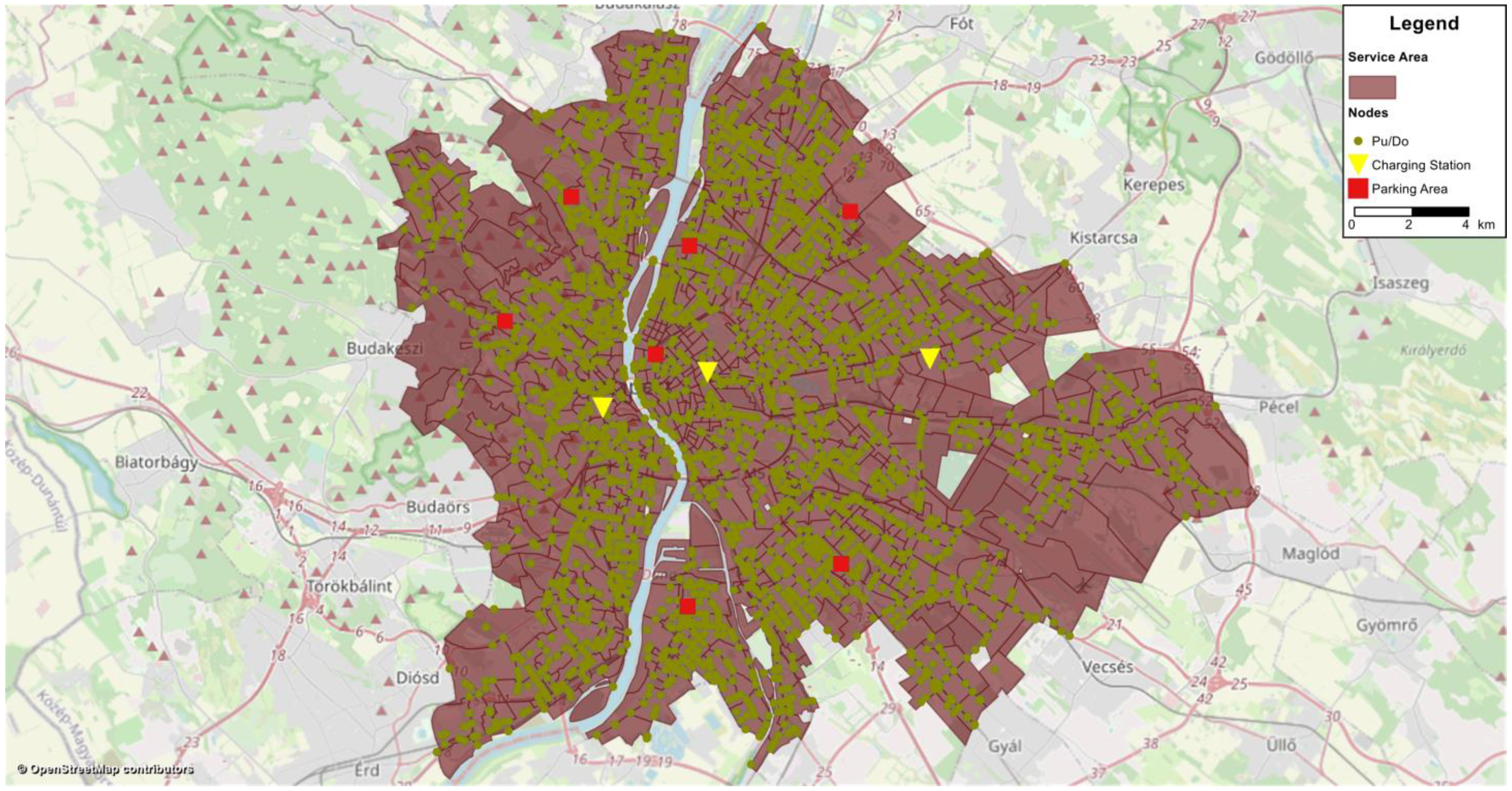
2.3.1. Conceptual Framework of the Simulation of an SAV System

The operation of DRS for SAVs starts when a user requests a trip at a certain location and time. The trip requests are then assigned to the SAV, which goes to the closest loading/unloading point rather than the exact location of the trip request. Similarly, the users would be provided with directions from their location to the closest loading point; noting that, from the SAV’s and user’s location to the loading point, the search of shortest path is executed. The assigned SAV must arrive at the loading point within the maximum arrival time calculated by Equation (6):

$$\mathit{Maximum}\mathit{ }\mathit{AT}\mathit{=}\mathit{EDT}\mathit{+}\mathit{IDT}\mathit{+}\mathit{MIN}\mathit{ }\mathit{\left(}\mathit{MAX}\mathit{ }\mathit{\left(}\mathit{\right(}\mathit{DF}\mathit{-}\mathit{1}\mathit{)}\mathit{ }\mathit{*}\mathit{ }\mathit{IDT}\mathit{,}\mathit{ }\mathit{ADT}\mathit{)}\mathit{,}\mathit{ }\mathit{MDT}\mathit{\right)}$$

(6)

where the arrival time is represented by $\mathit{AT}$, the earliest departure time is $\mathit{EDT}$, the ideal travel time is $\mathit{IDT}$, the detour factor is $\mathit{DF}$, the acceptable detour time is $\mathit{ADT}$, and the maximum detour time is $\mathit{MDT}$.

The detour factor is calculated by dividing the real (including detouring) travel time by the ideal (excluding detouring) travel time, with a maximum detour factor of 2, a maximum detour duration of 30 min, and a usually acceptable detour time of 10 min.

Users get into the SAV if it meets the maximum arrival time constraint and arrives at the loading point. Using the shortest path, the SAV leaves for the closest loading point to the final user destination while continuing to look for trip requests considering the capacity of the SAV, the accepted detour factor, and power constraints. When the passengers exit the SAV at the closest unloading point, they walk to their final destination and the SAV continues driving to the next loading/unloading point, using the shortest path.

Before each assignment, the electric power level in SAVs is checked to guarantee that they will be able to finish the assigned trips smoothly, with a maximum range of 150 km per charge for a four-seat SAV. If this is not the case, the SAV would be sent to the closest charging point. Similarly, if a car is idle for more than 30 min, it will also be directed to the closest charging point or car parking place.

2.3.2. Supply Modeling of SAV

Infrastructure and SAV fleet size are included in the supply modeling of DRS of SAVs. Defining the service area of SAVs in the network, parking spaces, charging points, and loading/unloading points are all part of the infrastructure supply modeling process. Similarly, the SAV fleet supply modeling entails defining the fleet size of SAVs and their features, on-road behaviors, and interactions with other automobiles. The rest of this section explains the most significant aspects of supply modeling in more detail.

The SAV service area is 475 km² in Budapest and contains 906 zones. Most of these zones, which consist of inner-city zones, have a medium to high demand intensity. Throughout operating, SAVs are allowed to exit the allocated zone; however, loading/unloading of passengers is only permissible within the defined zone of the SAV service area.

Passengers and SAVs can travel on allowed walking paths and private vehicle links, respectively, but not alternative types of links. Visum’s function walking transport mode [DRT Walk] was used to distinguish the walking routes of passengers from their location to the loading point and from the unloading point to their end location.

Inside the SAV service area, accessible loading/unloading points by walking and private vehicles were constructed at 1979 points. Despite users’ preference for door-to-door service, our model simulation environment does not enable it, necessitating the creation of loading/unloading points over the network.

The fleet size (i.e., the number of active and idle SAVs) should be identified to efficiently meet the users’ trip requests. Accordingly, in each scenario, the optimum SAV fleet size required to meet the demand of the generated trip requests inside the service area during the AP was identified by running a warm-up simulation consisting of twenty different random seed values of the function “Generate Trip Request and Tour Planning Procedures”. This approach yielded twenty different numbers for the necessary fleet size; additionally, these values represent the number of trip requests and their spatial-temporal randomness. In each scenario, the average of these values, obtained from the warm-up simulation, was used to calculate the size of the SAV fleet, which was 1100, 1640, and 4387 in the Mix-Traffic scenario, in the AV-Focused scenario, and the SAV-Focused scenario, respectively.

Various studies predicted a decrease in the necessary car parking slots, notably in the city center, with the emergence of SAVs [38], so parking spaces were assigned at seven nodes (already existing parking locations in Budapest) inside the service area. As stated before, the SAV fleet is entirely comprised of electric vehicles. As a result, charging stations were installed at 10 points throughout the service area, primarily at parking spaces, petrol stations, and established electric vehicle charging sites. Additionally, before the assignment, the charging period and power status of the battery are checked; charging the battery from 0 to 80 percent requires 4 h, and from 80 percent to 100 percent needs 3 h. Carrying an optimization to assign the SAV facilities locations, comprising charging stations, parking spaces, and loading/unloading points, is necessary to enable more efficient servicing of the SAV fleet; it can be carried out using the Capacitated Facility Location Problem (CFLP). Nevertheless, because implementing such an application would broaden the study area, this constraint is left for a subsequent study. Figure 1 depicts the SAV’s service area, the loading/unloading points as well as the charging facilities and parking spaces.

The adopted SAV model in this research depends on a real-time sharing system. In other words, the dispatcher receives only the spatiotemporal information about the trip requests when a passenger requests a trip, noting that booking an SAV in advance is not possible here. Therefore, a module that allows dynamic online dispatching is required. The vehicle routing problem (VRP) is suitable in this case as it provides the possibility of dynamically serving the maximal number of trip requests by utilizing the SAV fleet [39]. The VRP module was deployed within the tour planning procedure in Visum, which connects the generated trip requests (demand), SAV fleet (supply), and SAV infrastructure (loading/unloading point, parking, and charging areas) for the dispatching process. Various constraints were considered while executing the tour planning procedure; some of them were addressed before in this section, including vehicle capacity, charging duration of the battery, maximum detour factor and time, maximum range per charge, and inactive time. Other constraints were related to passengers, including the maximum allowed waiting time as well as desired pick-up and arrival time. All these constraints were considered within the assignment process.

3. Proposed Future Traffic Scenarios

This study compared the impact of the emergence of AVs and SAVs on traffic and CS in three distinct future traffic scenarios to the Base scenario. The alternative future scenarios seek to encompass the different possibilities for the advent of AVs and SAVs in Budapest in the years 2030 and 2050. The future scenarios’ travel demand was derived from BKK predictions for the relevant years. The overall predicted demand stayed the same; however, a change took place by substituting CC in the private travel demand with the assumed proportion of AV and SAV in each scenario. The creation of O-D matrices for AVs and SAVs was accomplished by multiplying every cell in the O-D matrix of private travel demand by the relevant diffusion percentages for AV and SAV in every scenario considering their service area zones. Simultaneously, the proportion of CC in the private travel demand matrix was reduced by the same percentage as the diffusion percentages of AV and SAV. In the years 2020, 2030, and 2050, the total predicted private travel demand was 2.16, 2.23, and 2.31 million trips per day, respectively. Although the modal shift may occur from various modes of transport like PuT and cycling, this study examined the effect of substituting CC in the private travel demands with AV and SAV while assuming the modal split stays the same and comparing the results to the Base scenario in terms of traffic performance and CS.

The first scenario, Base scenario, utilizes the expected private travel demand for Budapest in 2020 without including AVs or SAVs. For pragmatic reasons, the expected travel demand for the year 2020 was chosen above the actual travel demand, which was markedly reduced as a result of the COVID-19 pandemic and restrictions applied; thus, rather than compare such low travel demand with much higher ones for the year 2030 and 2050, we used the projections of private travel demand in all investigated scenarios that would provide more consistency in the results. The Mix-Traffic scenario is the second scenario, which uses the forecasted travel demand for Budapest in 2030 and blends CC, AV, and SAV modes. By 2030, it is projected that self-automated vehicles will be on the roads [4], and passengers may switch to AV and SAV. However, owing to their expected initial high prices, the adoption of automated vehicles might be limited [2,40]. As a result, in this scenario, the primary mode of private transport is CC, which accounts for 50 percent of private travel demand, trailed by AV and SAV, which account for 40 and 10 percent of demand, respectively. The simulated region depicted in Figure 2 reflects Budapest and its vicinity.

Full substitution of CCs by AVs and SAVs was assumed in the second and third scenarios, where BKK’s predicted travel demand for Budapest in 2050 was utilized in the simulation procedure. Many studies anticipated that AVs would completely or largely replace CCs by 2050 [1,3]. The relative distribution of AVs and SAVs, on the other hand, is still unclear, as is which of these two future modes will become the dominant transport mode [15]. Thus, two alternative scenarios were created to reflect the two possibilities for the introduction of AVs and SAVs. In the AV-Focused scenario, CCs in Budapest’s private travel forecasted demand for 2050 were replaced by AVs and SAVs, with AVs accounting for 85 percent and SAVs for 15 percent. In this scenario, it is assumed that the majority of vehicle owners and those with access to private vehicles will change from CCs to privately owned AVs, with just 15 percent switching to SAVs. Contrarily, in the SAV-Focused scenario, the SAV mode is considered to be easily obtainable, widely available, and has a high adoption rate of 40 percent of private travel demand, compared to 60 percent for the AV mode. SAV fleets are projected to operate on city streets in the near future to accommodate travel demand, as ride-hailing companies spend heavily on establishing SAV fleets in cities as an alternate form of transportation [41]. Chen & Kockelman [11] anticipated that a fleet of electric SAVs might account for between 14 and 39 percent of the mode share in a mid-sized city under specific conditions. Based on these results, the expected penetration rates of SAVs for the second and third scenarios were chosen as 15 and 40 percent, respectively. The rest were assigned to AV mode.

4. Results and Discussion

The findings reported in this section show the influence of the introduction of AVs and SAVs on TPP and the change in CS in the proposed future traffic scenarios compared to the Base scenario. The examined TPPs are average and max queue length, delay, volume, density, utilization, velocity, and VKT. The following paragraphs explain each of these parameters and the change in CS.

The SBA queue length outputs show the average and maximum queue lengths (lane average and lane max) on the link edges assigned to lanes in meters at each analysis time interval (ATI). It is derived by multiplying the average accumulated vehicle length on the lane during the ATI by the proportion of time spent waiting for vehicles at the end of a lane divided by the ATI. The effect of implementing AVs and SAVs in the network on average and maximum queue lengths differs according to their penetration rates. Considering the summation of average queues accumulated on each link in the network for every scenario shows that the highest value occurred at 8:00 AM in the Base scenario, where the summation of average queues was 60 km. This value decreased significantly, when deploying AVs and SAVs in the road network by 78%, 93%, and 99% for Mix-Traffic, AV-Focused, and SAV-Focused scenarios, respectively. SBA handles queues dynamically and passes on congested vehicles to the next time interval; in the case of the last ATI, the queue would be dissolved in the extension time interval. Noting that the smaller SBA reaction time parameter changes the behavior of following vehicles by reducing the headways; consequently, more vehicles can pass over a link in one hour before queues form.

The SBA max queue length shows the maximum queue length accumulated on each link at each ATI. Figure 3 depicts the summation of the average queue length on the left y-axis and the maximum of the SBA max queue length on the right y-axis for each scenario in the whole network at 8:00 AM. The maximum of max queue length (i.e., the longest queue occurred in the network at 8:00 AM in every scenario) followed a similar pattern to average queue length, where it decreased by 44%, 45%, and 95% in Mix-Traffic, AV-Focused, and SAV-Focused scenarios, respectively. In a wider perspective, the percentage change in the summation of SBA max queue lengths on all links in the network yields again a similar pattern of the change in the summation of average queue length with approximately the same percentages.

The SBA calculates delay by comparing the travel time in a network with no volume (t₀) to the average travel time when the volume is taken into account (t_cur) during the AP. Figure 4 shows the percentage changes in delay due to the emergence of AVs and SAVs into the road network for each scenario. The percentage change in delay illustrates that deploying self-driving vehicles into the road network significantly reduced the delays. In the Mix-Traffic scenario, the delays were decreased by 77%, and a further reduction took place in AV-Focused and SAV-Focused scenarios at 94% and 97%, respectively. The reason behind such reduction refers to the reduction in queue lengths, which implied that vehicle waiting times at the end of the links was much smaller. Additionally, the reduction in traffic volumes as a smaller number of SAVs replaced many CCs, which resulted in fewer traffic volumes on the links and smaller difference between t₀ and t_cur, consequently reducing the delays. It was noticed that the emergence of AVs and SAVs in the network reduced the summation of average queue lengths and the delays by almost the same percentage in every scenario.

The SBA calculates the volume for each link in the network as the count of vehicles that crossed the network links during the AP [Veh/h]. Although implementing Avs would cause shorter headways, which would most likely generate more capacity due to better utilization of the roads, resulting in more vehicles passing through a certain point within a certain time unit (i.e., capacity), the traffic volume decreased in the investigated future traffic scenarios. The reason behind this reduction is associated with replacing CCs with SAVs. In the Mix-Traffic, AV-Focused, and SAV-Focused scenarios, 1100, 1640, and 4387 SAVs served 15,945, 24,775, and 66,066 trips of private travel demand during the AP, respectively. Figure 5 shows the total volume in the network in all scenarios during the AP and the percentage reduction in the volume for the proposed future traffic scenarios compared to the Base scenario. The volume decreased with increasing the penetration rate of AVs and SAVs, and the maximum reduction was reached in the SAV-Focused scenario at 45%.

SBA density is a simulation’s output that refers to the average number of vehicles per kilometer on the link during ATI. Similar to the previously investigated TPPs (i.e., queue length, delay, and volume), the density was reduced when including AVs and SAVs in the simulation procedure. The reduction in average traffic density during the AP compared to the Base scenario was 16%, 25%, and 55% for the Mix-Traffic, AV-Focused, and SAV-Focused scenarios, respectively. Figure 6 illustrates the reduction in average density resulting from the emergence of AVs and SAVs during AP at each ATI. It is evident that a higher replacement rate of CCs by SAVs affected the average density more; for instance, the average traffic density at 8:00 AM in the Base scenario was 5.8 [Veh/km], and it was reduced to 4.2, 3.4, and 2 [Veh/km] for the Mix-Traffic, AV-Focused and SAV-Focused scenarios, respectively.

SBA utilization is an output attribute obtained during the simulation and corresponding to scaled density. It shows how much of the link’s capacity is being used based on the fundamental diagram, which connects volume and density values. A visualization of the SBA utilization attribute at 8:00 AM that compared the three proposed future traffic scenarios to the Base scenario is depicted in Figure 7. The green color in the figure illustrates less traffic on the links allowing more cars to use it until reaching the critical density; hence utilization is improved, whereas the red color shows the opposite. The most significant effects on utilization occurred in the city center and on the ring around Budapest in all scenarios, with a noticeable increase in the green color and diminishing red color as the replacement rate of CCs by AVs and SAVs increases. The comparison showed that the maximum improvement in the network took place in the SAV-Focused scenario, followed by AV-Focused and Mix-Traffic scenarios.

SBA velocity attribute is calculated from SBA length, including the vehicle and the link lengths, and the average travel time of vehicles that crossed the link during the AP. Then, the average velocity of all vehicles that used that link is sorted in Visum as a link attribute. The average vehicles’ velocity in the whole network (i.e., the average of all link’s average velocities) increased with the advent of the AVs and SAVs. The average vehicles’ velocity for all links in the network and the percentage increment in the velocity in the future traffic scenarios compared to the Base scenario are depicted in Figure 8. The velocity increased with the emergence of AVs and SAVs by 2% in the Mix-traffic scenario, 4% in the AV-Focused scenario, and more increment took place in the SAV-Focused scenario to reach 5% compared to the Base scenario.

In reference to the Base scenario, the results revealed that VKT increased in the Mix-Traffic scenario by 18%. On the contrary, it decreased in the AV-Focused scenario by 2%, and by 36% in the SAV-Focused scenario. The reduction in the VKT was associated with the reduction in the volume. It is worth mentioning that if the boarding passengers in SAV have the same destination, the trip is considered one trip. Otherwise, passengers with different destinations are considered as several trips. For example, if two passengers board together and head towards the same destination, this is counted as one trip of the demand. However, if these two passengers have two different destinations, they are counted as two trips of demand. This shows the effect of SAVs on reducing the number of private transport trips by personal car through applying the DRS to serve the private travel demand. However, one of the major characteristics of self-driving vehicles is the ability to drive unoccupied [42], and this aspect was investigated here. The total VKT by SAVs increased with the increment in the share distribution of SAVs, where more than 96% of VKT, which SAVs covered in every scenario, were occupied trips.

Table 2. VKT [km] in the network during AP.

VKT [km]	Base	Mix-Traffic	AV-Focused	SAV-Focused
Total VKT	17,228,943	20,510,993	16,923,120	10,991,717
Total VKT by SAV	-	82,673	128,518	466,572
Occupied VKT	-	79,629	124,094	453,275
Unoccupied VKT	-	3044	4424	13,297

shows all scenarios’ total, occupied, and unoccupied VKT in kilometers.

A statistical analysis of the acquired data was utilized to find the significant differences between the three proposed future traffic scenarios (Mix-Traffic, AV-Focused, and SAV-Focused) and the Base scenario for each parameter in the TPPs described above. Friedman and Wilcoxon signed-rank tests (non-parametric tests) were used to compare future traffic scenarios to the Base scenario since the data did not fit a normal distribution. The Friedman test with Bonferroni correction revealed that the distribution of all TPPs among the possible combinations (i.e., Mix-Traffic–Base, AV-Focused–Base, and SAV-Focused–Base) is not the same.

For pairwise comparisons, the Wilcoxon signed-rank test was used for all pairings that had different distributions according to the Friedman test. The results showed a significant difference for all TPPs in the investigated combinations (p < 0.001).

Table 3. Wilcoxon signed-rank test results for investigated TPP.

TPP	Mix-Traffic–Base		AV-Focused–Base		SAV-Focused–Base
	Z	r	Z	r	Z	r
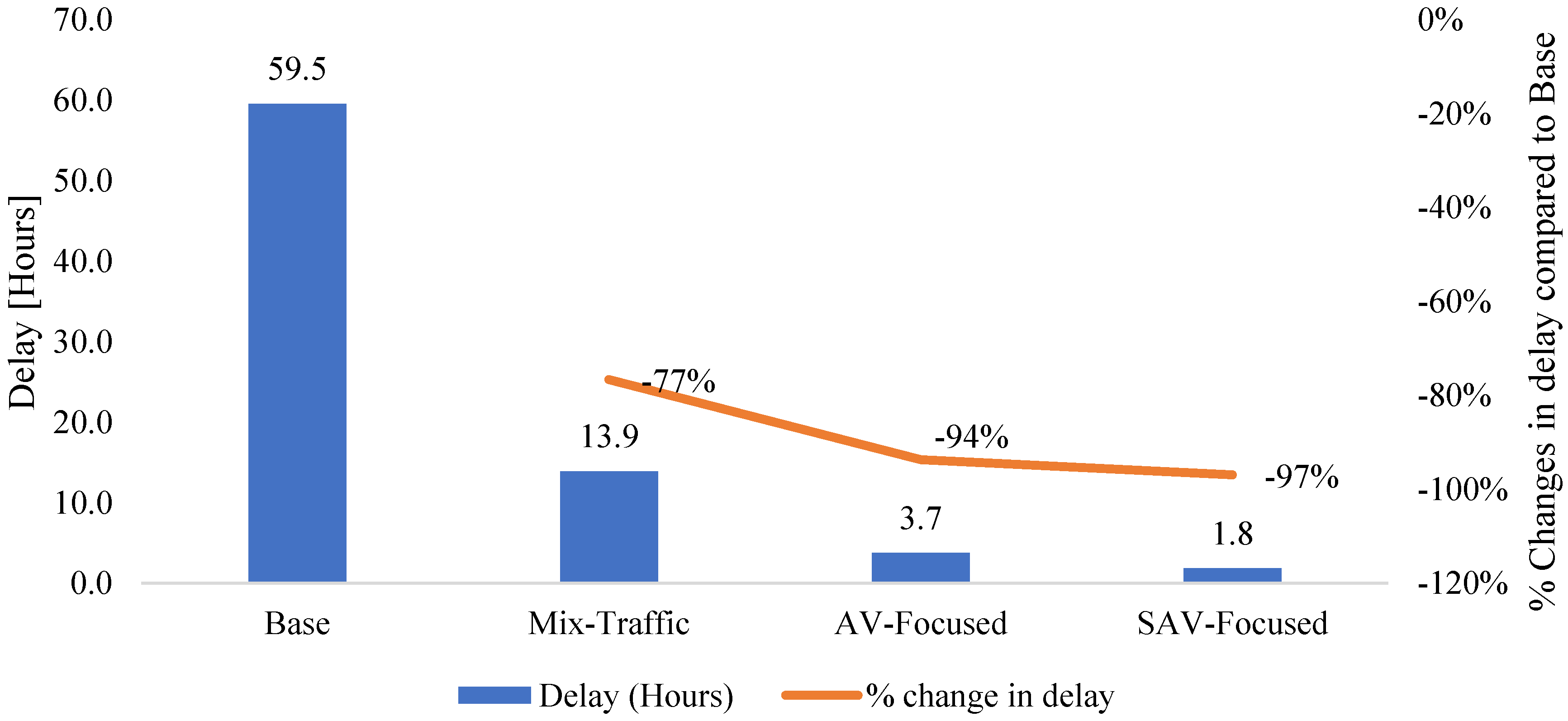
Delay	−19.940 a	0.11	−52.255 a	0.30	−60.033 a	0.34
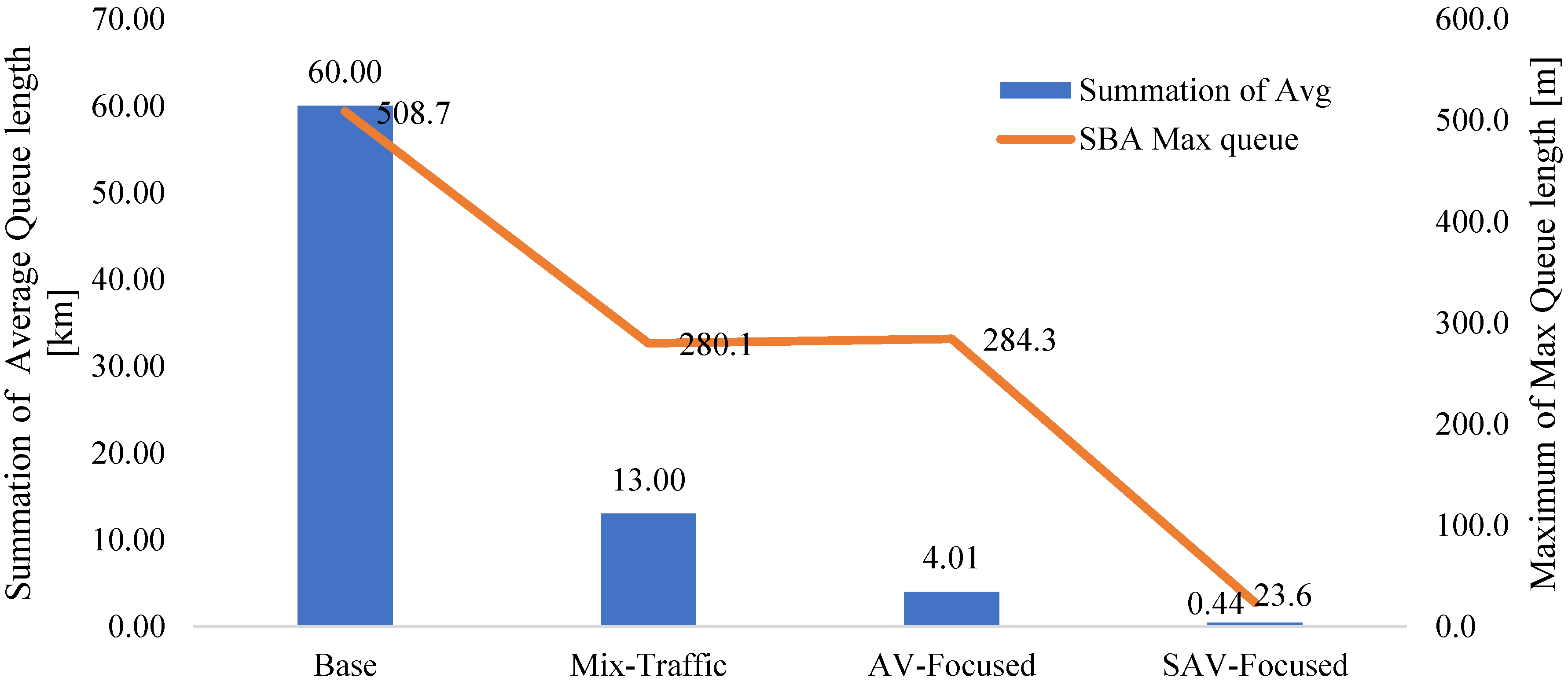
Average Queue Length	−26.792 a	0.15	−48.064 a	0.28	−64.769 a	0.37
Max Queue Length	−26.359 a	0.15	−47.633 a	0.27	−64.388 a	0.37
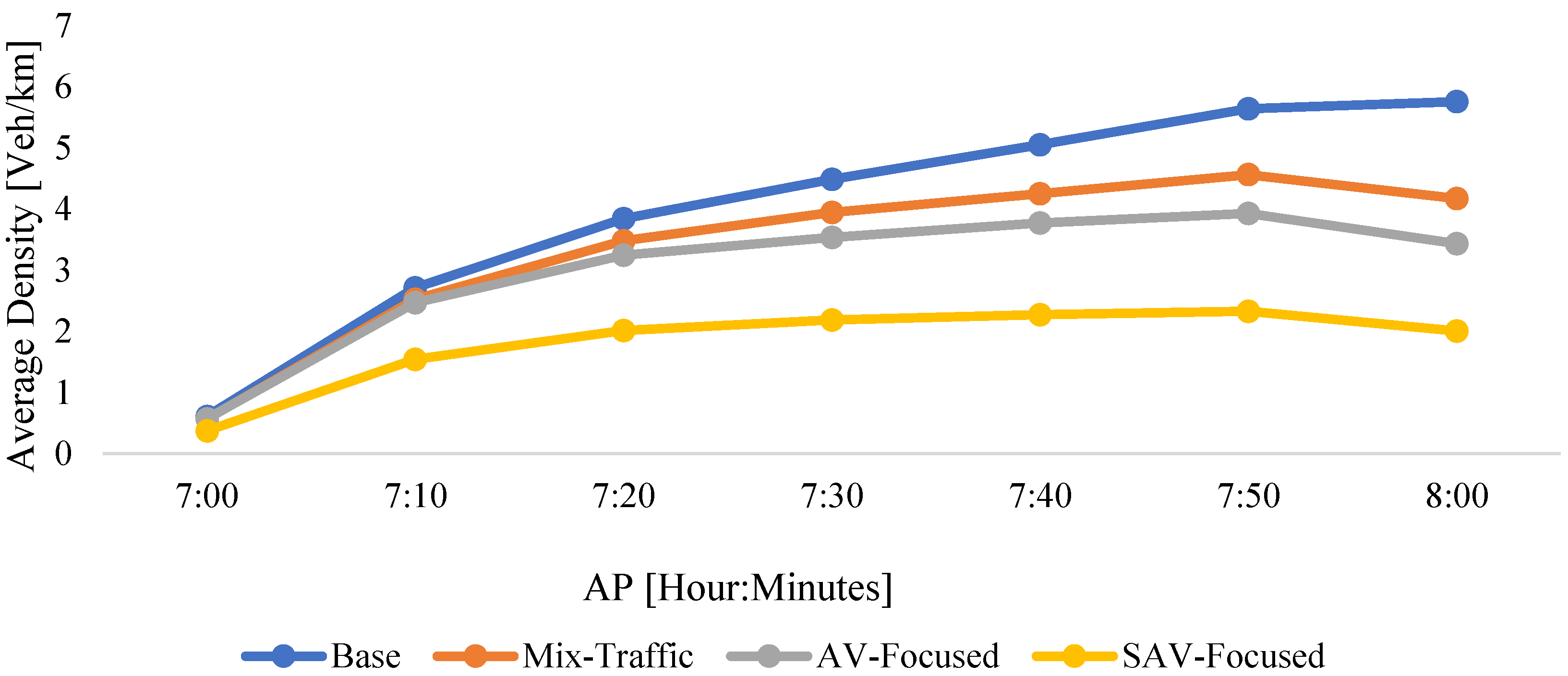
Average Density	−20.623 a	0.12	−42.973 a	0.25	−98.263 a	0.56
Volume	−76.876 a	0.44	−78.007 a	0.45	−112.498 a	0.65
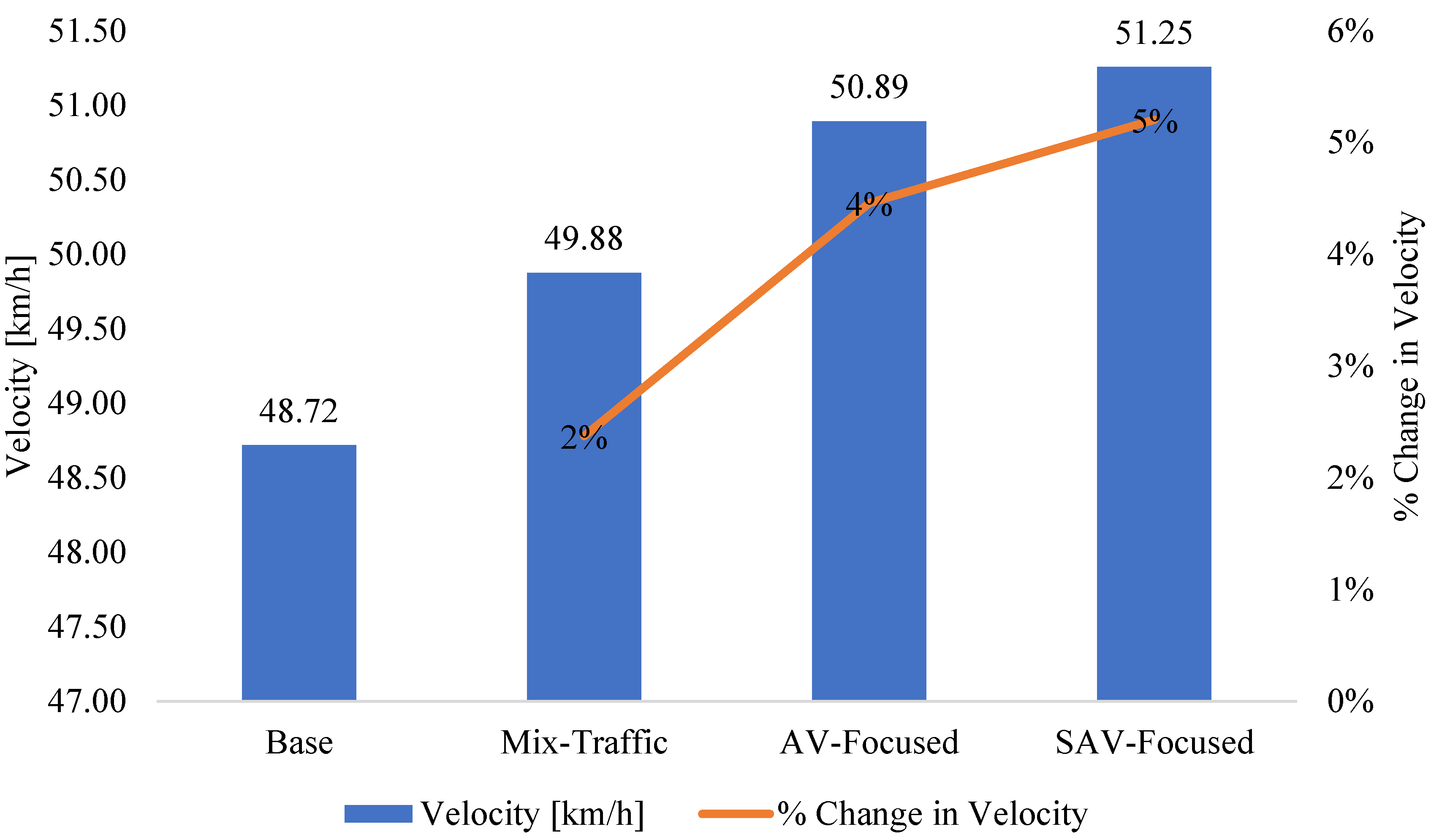
Average Velocity	−41.129 b	0.24	−56.012 b	0.32	−60.978 b	0.35
VKT	−69.995 b	0.40	−30.744 a	0.18	−102.861 a	0.59

Note: ^a. Based on positive ranks (p < 0.001); ^b. Based on negative ranks (p < 0.001).

shows the Z-values and effect sizes (r) obtained by dividing the z value by the square root of observations (N). The effect size increased with the increment in AV and SAV share distribution; moreover, higher values for (r) were noticed in the SAV-Focused scenario. Exceptions were found in the case of (AV-Focused scenario–Base scenario) for VKT, where the effect size had a smaller value than in (Mix-Traffic scenario–Base scenario).

The user’s benefit (i.e., CS) resulting from the emergence of AVs and SAVs is displayed in Figure 9. It can be noticed that the emergence of AVs and SAVs caused a positive change in CS in all scenarios. The increased CS is reasonable considering the lower assumed VOTT for AVs and SAVs in this research. The highest increment in the CS occurred in the AV-Focused scenario, and the positive change in CS was approximately the same in Mix-Traffic and SAV-Focused scenarios.

5. Conclusions

The introduction of AVs and SAVs into the transportation sector is anticipated to provide several benefits with regard to the road network. However, the share distribution of AV and SAV is not yet evident. Therefore, three alternative future traffic scenarios reflecting various AV and SAV emergence possibilities were devised to explore the potential consequences of varying AV and SAV penetration rates on the network performance and total change in CS in the city of Budapest.

In the modeling procedure for the Base and future traffic scenarios, the forecasted travel demands for Budapest for the years 2020, 2030, and 2050 were used. The future traffic scenarios consisted of the inclusion of CCs, AVs, and SAVs for 2030 in the Mix-Traffic scenario and the replacement of all trips made with CCs by AV and SAV modes for 2050 in the other two scenarios. This included two separate approaches: (1) AVs were considered to be widely utilized as a private self-driving vehicle in the AV-Focused scenario, and (2) SAVs were assumed to be largely used in the SAV-Focused scenario. The simulation was carried out using the SBA with Visum software based on an existing and validated traffic model, the EFM Model.

The utilization of a professionally designed and calibrated EFM model; deploying SBA in the network loading process within the assignment and involving the forecasted travel demand of the investigated years (2020, 2030, and 2050) in the analysis allow for more stable results in terms of network performance and changes in CS. In addition, the DRS was used to model the SAV system, taking into account several essential qualities that are predicted in SAV structures, such as in-route check and acceptance of other trip requests based on detour factor, the vehicle power level and recharge, and time constraints for the vehicle to pick-up a request. However, this research can be further extended by overcoming some limitations. In this study, only private transportation modes are taken into account while analyzing the implications of the emergence of AVs and SAVs; therefore, this research can be expanded to examine the impact of such emergence on the mobility behavior of people, such as mode choice. As mentioned earlier, VOTT can be assigned for different categories of users and based on trip purpose. Similarly, using an optimization method to determine the locations of the SAV facilities, including loading/unloading points, charging stations, and parking spaces would allow more efficient application of the SAV fleet.

The results show that the advent of AVs and SAVs in the Budapest network will enhance the TPPs and increase the CS. The network performance witnessed additional improvements with a higher replacement rate of CCs by SAVs, where the lowest queue lengths, minimum delays, maximum velocities, and lowest VKT took place in the SAV-Focused scenario, followed by AV-Focused and Mix-Traffic scenarios, respectively. Similarly, the CS increased in all future scenarios, especially with increasing the share distribution of AVs (i.e., AV-Focused scenario). Hence, road users and authorities will benefit from the emergence of AVs and SAVs; however, a higher replacement rate of CCs by SAVs will have a more positive impact on traffic status, while a higher replacement rate of CCs by AVs will increase road user’s benefits. The improved network performance might induce additional travel demand, which may necessitate applying travel demand management like road pricing [43,44]; this aspect was not analyzed here as it falls beyond the research scope. Moreover, this research analyzed the implications of replacing CCs with AVs and SAVs in alternative future scenarios while assuming no changes would occur in the modal share; however, it could be interesting for future research to broaden the research area to cover the impact of AVs and SAVs on the public’s mobility behavior, mode choice, and the possibility that a great part of mobility could involve public transport.

References

- Litman, T. Autonomous Vehicle Implementation Predictions: Implications for Transport Planning; Victoria Transport Policy Institute: Victoria, BC, Canada, 2020; p. 45. [Google Scholar]
- Webb, J.; Wilson, C.; Kularatne, T. Will People Accept Shared Autonomous Electric Vehicles? A Survey before and after Receipt of the Costs and Benefits. Econ. Anal. Policy 2019, 61, 118–135. [Google Scholar] [CrossRef]
- Bansal, P.; Kockelman, K.M. Forecasting Americans’ Long-Term Adoption of Connected and Autonomous Vehicle Technologies. Transp. Res. Part A Policy Pract. 2017, 95, 49–63. [Google Scholar] [CrossRef]
- Kockelman, K.; Boyles, S.; Stone, P.; Fagnant, D.; Patel, R.; Levin, M.W.; Guni, S.; Simoni, M.; Albert, M.; Fritz, H.; et al. An Assessment of Autonomous Vehicles: Traffic Impacts and Infrastructure Needs—Final Report; University of Texas at Austin. Center for Transportation Research: Austin, TX, USA, 2017. [Google Scholar] [CrossRef]
- Autovista Group. The State of Autonomous Legislation in Europe. Available online: https://autovistagroup.com/news-and-insights/state-autonomous-legislation-europe (accessed on 20 May 2020).
- Ferrero, F.; Perboli, G.; Rosano, M.; Vesco, A. Car-Sharing Services: An Annotated Review. Sustain. Cities Soc. 2018, 37, 501–518. [Google Scholar] [CrossRef]
- Hall, J.V.; Krueger, A.B. An Analysis of the Labor Market for Uber’s Driver-Partners in the United States. ILR Rev. 2018, 71, 705–732. [Google Scholar] [CrossRef]
- Chen, T.D.; Kockelman, K.M. Carsharing’s Life-Cycle Impacts on Energy Use and Greenhouse Gas Emissions. Transp. Res. Part D Transp. Environ. 2016, 47, 276–284. [Google Scholar] [CrossRef]
- Martin, E.W.; Shaheen, S.A. Greenhouse Gas Emission Impacts of Carsharing in North America. IEEE Trans. Intell. Transp. Syst. 2011, 12, 1074–1086. [Google Scholar] [CrossRef]
- Matalqah, I.; Shatanawi, M.; Alatawneh, A.; Mészáros, F. Impact of Different Penetration Rates of Shared Autonomous Vehicles on Traffic: Case Study of Budapest. Transp. Res. Rec. 2022, 03611981221095526. [Google Scholar] [CrossRef]
- Chen, T.D.; Kockelman, K.M. Management of a Shared Autonomous Electric Vehicle Fleet: Implications of Pricing Schemes. Transp. Res. Rec. 2016, 2572, 37–46. [Google Scholar] [CrossRef]
- Meszaros, F.; Shatanawi, M.; Ogunkunbi, G.A. Challenges of the Electric Vehicle Markets in Emerging Economies. Period. Polytech. Transp. Eng. 2020, 49, 93–101. [Google Scholar] [CrossRef] [Green Version]
- Krueger, R.; Rashidi, T.H.; Rose, J.M. Preferences for Shared Autonomous Vehicles. Transp. Res. Part C Emerg. Technol. 2016, 69, 343–355. [Google Scholar] [CrossRef]
- Fagnant, D.J.; Kockelman, K. Preparing a Nation for Autonomous Vehicles: Opportunities, Barriers and Policy Recommendations. Transp. Res. Part A Policy Pract. 2015, 77, 167–181. [Google Scholar] [CrossRef]
- Simoni, M.D.; Kockelman, K.M.; Gurumurthy, K.M.; Bischoff, J. Congestion Pricing in a World of Self-Driving Vehicles: An Analysis of Different Strategies in Alternative Future Scenarios. Transp. Res. Part C Emerg. Technol. 2019, 98, 167–185. [Google Scholar] [CrossRef]
- Van den Berg, V.A.C.; Verhoef, E.T. Autonomous Cars and Dynamic Bottleneck Congestion: The Effects on Capacity, Value of Time and Preference Heterogeneity. Transp. Res. Part B Methodol. 2016, 94, 43–60. [Google Scholar] [CrossRef]
- Shatanawi, M.; Ghadi, M.; Mészáros, F. Road Pricing Adaptation to Era of Autonomous and Shared Autonomous Vehicles: Perspective of Brazil, Jordan, and Azerbaijan. Transp. Res. Procedia 2021, 55, 291–298. [Google Scholar] [CrossRef]
- Wadud, Z.; MacKenzie, D.; Leiby, P. Help or Hindrance? The Travel, Energy and Carbon Impacts of Highly Automated Vehicles. Transp. Res. Part A Policy Pract. 2016, 86, 1–18. [Google Scholar] [CrossRef]
- Milakis, D.; van Arem, B.; van Wee, B. Policy and Society Related Implications of Automated Driving: A Review of Literature and Directions for Future Research. J. Intell. Transp. Syst. 2017, 21, 324–348. [Google Scholar] [CrossRef]
- Russo, F.; Rindone, C. Regional Transport Plans: From Direction Role Denied to Common Rules Identified. Sustainability 2021, 13, 9052. [Google Scholar] [CrossRef]
- Banister, D. The Sustainable Mobility Paradigm. Transp. Policy 2008, 15, 73–80. [Google Scholar] [CrossRef]
- Rindone, C. Sustainable Mobility as a Service: Supply Analysis and Test Cases. Information 2022, 13, 351. [Google Scholar] [CrossRef]
- ADAC. The Evolution of Mobility; ZukunftsInstitut: Frankfurt am Main, Germany, 2018; p. 45. Available online: https://www.adac.de/-/media/pdf/dko/adac-studie-evolution-der-mobilitaet-englisch.pdf (accessed on 27 July 2022).
- Hungarian Central Statistical Office. Available online: https://www.ksh.hu/?lang=en (accessed on 28 December 2021).
- Department for Transport. TAG UNIT M3.1. Highway Assignment Modelling; Department for Transport: London, UK, 2020; p. 76.
- Főmterv Ltd.; Közlekedés Ltd.; Trenecon Ltd. Egységes Forgalmi Modell; Centre for Budapest Transport: Budapest, Hungary, 2015; p. 71. [Google Scholar]
- PTV Group. PTV Visum Online Manual. Available online: https://cgi.ptvgroup.com/vision-help/VISUM_2021_ENG/Content/TitelCopyright/Index.htm (accessed on 28 December 2021).
- Maciejewski, M.; Bischoff, J. Congestion Effects of Autonomous Taxi Fleets. Transport 2018, 33, 971–980. [Google Scholar] [CrossRef]
- Mahmassani, H.S. Dynamic Network Traffic Assignment and Simulation Methodology for Advanced System Management Applications. Netw. Spat. Econ. 2001, 1, 267–292. [Google Scholar] [CrossRef]
- Ahmed, A. Integration of Real-Time Traffic State Estimation and Dynamic Traffic Assignment with Applications to Advanced Traveller Information Systems. Ph.D. Thesis, University of Leeds, Leeds, UK, 2015. [Google Scholar]
- Matrai, T.; Abel, M.; Kerenyi, L.S. How Can a Transport Model Be Integrated to the Strategic Transport Planning Approach: A Case Study from Budapest. In Proceedings of the 2015 International Conference on Models and Technologies for Intelligent Transportation Systems (MT-ITS), Budapest, Hungary, 3–5 June 2015; pp. 192–199. [Google Scholar]
- Berki, Z. Tackling Sustainable Urban Transport Policy Measures in Transport Models. In Proceedings of the 2015 International Conference on Models and Technologies for Intelligent Transportation Systems (MT-ITS), Budapest, Hungary, 3–5 June 2015; pp. 356–361. [Google Scholar]
- Chiu, Y.; Bottom, J.; Mahut, M.; Paz, A.; Balakrishna, R.; Waller, T.S.; Hicks, J. Dynamic Traffic Assignment: A Primer; Transportation Research Board of the National Academies: Washington, DC, USA, 2011. [Google Scholar]
- Sundaram, S.; Koutsopoulos, H.N.; Ben-Akiva, M.; Antoniou, C.; Balakrishna, R. Simulation-Based Dynamic Traffic Assignment for Short-Term Planning Applications. Simul. Model. Pract. Theory 2011, 19, 450–462. [Google Scholar] [CrossRef]
- Vadali, S.; Kruse, C.J.; Kuhn, K.; Goodchild, A. Guide for Conducting Benefit-Cost Analyses of Multimodal, Multijurisdictional Freight Corridor Investments; Transportation Research Board: Washington, DC, USA, 2017; p. 24680. ISBN 978-0-309-45545-9. [Google Scholar]
- Winkler, C. Transport User Benefits Calculation with the “Rule of a Half” for Travel Demand Models with Constraints. Res. Transp. Econ. 2015, 49, 36–42. [Google Scholar] [CrossRef]
- Weiss, J.; Hledik, R.; Lueken, R.; Lee, T.; Gorman, W. The Electrification Accelerator: Understanding the Implications of Autonomous Vehicles for Electric Utilities. Electr. J. 2017, 30, 50–57. [Google Scholar] [CrossRef]
- Zhang, W.; Guhathakurta, S.; Fang, J.; Zhang, G. Exploring the Impact of Shared Autonomous Vehicles on Urban Parking Demand: An Agent-Based Simulation Approach. Sustain. Cities Soc. 2015, 19, 34–45. [Google Scholar] [CrossRef]
- Maciejewski, M.; Bischoff, J.; Hörl, S.; Nagel, K. Towards a Testbed for Dynamic Vehicle Routing Algorithms. In Proceedings of the Highlights of Practical Applications of Cyber-Physical Multi-Agent Systems; Bajo, J., Vale, Z., Hallenborg, K., Rocha, A.P., Mathieu, P., Pawlewski, P., Del Val, E., Novais, P., Lopes, F., Duque Méndez, N.D., Julián, V., Holmgren, J., Eds.; Springer International Publishing: Cham, Germany, 2017; pp. 69–79. [Google Scholar]
- Menon, N.; Barbour, N.; Zhang, Y.; Pinjari, A.R.; Mannering, F. Shared Autonomous Vehicles and Their Potential Impacts on Household Vehicle Ownership: An Exploratory Empirical Assessment. Int. J. Sustain. Transp. 2019, 13, 111–122. [Google Scholar] [CrossRef]
- Kang, C. No Driver? Bring It On. How Pittsburgh Became Uber’s Testing Ground. The New York Times, 14 September 2016. [Google Scholar]
- Cokyasar, T.; Larson, J. Optimal Assignment for the Single-Household Shared Autonomous Vehicle Problem. Transp. Res. Part B Methodol. 2020, 141, 98–115. [Google Scholar] [CrossRef]
- Shatanawi, M.; Abdelkhalek, F.; Mészáros, F. Urban Congestion Charging Acceptability: An International Comparative Study. Sustainability 2020, 12, 5044. [Google Scholar] [CrossRef]
- Shatanawi, M.; Alatawneh, A.; Mészáros, F. Implications of Static and Dynamic Road Pricing Strategies in the Era of Autonomous and Shared Autonomous Vehicles Using Simulation-Based Dynamic Traffic Assignment: The Case of Budapest. Res. Transp. Econ. 2022, 101231. [Google Scholar] [CrossRef]