Article

Assessment of the Usability of Some Bio-Based Insulation Materials in Double-Skin Steel Envelopes

1
Univ. Orleans, Univ. Tours, INSA-CVL, LaMé —EA7494, 8 Rue Léonard de Vinci, 45072 Orléans, France
2
Department of Transportation Infrastructure and Foundations, Faculty of Civil Engineering and Building Services, “Gheorghe Asachi” Technical University of Iași, 1 Prof. D. Mangeron St., 700050 Iași, Romania
3
Enveloppe Métallique du Bâtiment, 6/14 Rue la Pérouse, CEDEX 16, 75784 Paris, France
*
Author to whom correspondence should be addressed.
Sustainability 2022, 14(17), 10797; https://doi.org/10.3390/su141710797
Submission received: 14 June 2022 / Revised: 15 August 2022 / Accepted: 24 August 2022 / Published: 30 August 2022
(This article belongs to the Special Issue Studies on Sustainable Rehabilitation of the Built Environment)

Abstract

:
In this paper, a double-skin steel building-demonstrator, set up using panels of five bio-based insulators and a classical mineral insulating material, is studied. The panels used in the demonstrator are made from industrially manufactured and commercialized bio-materials. To assess the suitability of these panels for use in cold formed steel envelope buildings, their advantages and/or the drawbacks (if any) of the synchronized records of temperatures, relative humidity and thermal flux of each panel are obtained using a system of continuous measurements. Data from 6 months of records in the roof of the demonstrator are used to assess the infield properties of the panels and the seasonal evolution of these properties in relation to the presence of the vapor barrier. The thermal resistance of each panel is determined from these data using two methods: the ISO 9869-1:2014 based on the Heat Flow Meter (HFM) method and an inverse problem identification method. All bio-sourced panels manifest higher thermal resistance than the classical insulation system, whatever conditions of use with or without barrier vapor. The seasonal variations of thermal properties are attenuated when a vapor barrier is used. No risk for water condensation inside the bio-insulations is revealed so far.

1. Introduction

Since 2020, a European Union directive (2010/31/EU) requires all new buildings in the European Community to be virtually carbon-free. A near zero-carbon building is defined as a high energy efficiency structure that meets energy needs using renewable sources [1,2]. The thermal regulation in France (RE2020) implies, among other factors, the optimization of the carbon footprint of buildings warmed above 12 °C. Such objectives are obtained by an overall optimization of the design (building shape, orientation), constructive systems, materials and devices for energy control and production.
Nowadays, in context of energy market tensions, the design of performant thermal building envelopes represents a successful economic strategy for energy consumption reduction, conservation of natural resources and reduction of greenhouse gas effects. Indeed, as the thermal performance of the building affects the energy consumption, performant insulation is a cheap and widely available technology that saves energy and money, all by reducing CO2 emissions at the same time.
The insulating materials used in buildings work on the principle of trapping air in more or less confined space and providing barriers for heat transfer. Along with the mineral and synthetic insulating materials, such as polystyrene, polyester, glass wool, mineral wool, etc., more and more bio-based materials such as hemp, cellulose wadding, bio-fibers, wood fibers, recycled textiles, just to mention only some of them, are used nowadays as insulating materials in construction and renovation [3,4,5].
For a long time, mineral and synthetic insulating materials were almost the only ones used in buildings and were considered good cheap insulators. However, in the framework of worldwide efforts to minimize the human impact on climate change, and in the context of raw materials rarefication, alternative bio-based insulating materials are widely used nowadays. An effective insulation strategy is part of a holistic approach to sustainability, including among others, evaluation of critical factors such as performance, durability, health, wellbeing economic costs [6]. The adoption of low-carbon materials such as bio-based insulation, considered to be long-term carbon sinks, is one of efficient tools to be used to meet climate change goals [7].
Bio-based insulation offers the advantage of storing CO2 from the atmosphere throughout its lifetime, reducing the climatic impact [8], yet providing very interesting thermal properties compared to conventional insulation [9]. In addition, bio-based insulations are non-irritating and less polluting when it comes to waste management as they are biodegradable, making them more user-friendly.
Bio-based insulators assist in passive control of indoor air conditions for temperature and humidity through hygroscopicity [10]. In most cases, these insulators have a fibrous structure, which explains their regulator hygroscopic properties and high moisture buffering values [6,11,12,13].
However, because of these hygroscopic properties, these materials are also subject to a particular vigilance and monitoring because they represent a significant risk for liquid water condensation. In turn, water condensation could create favorable conditions for mold growth, insect and/or rodent activity that could be of concern for the health of habitants and/or for that of the structure [11,12,13].
Likewise, due to their inherent carbon-based chemical structure, the use of such insulators could be a source of volatile organic compounds (VOC) emission [14].
The bio-based insulating materials are also a response to the problem of rarefaction of raw materials [15,16]. Most often, the bio-based materials, such as wood fibers, textiles, straw fibers and so on, are secondary products of agriculture or various industries [1,17].
The durability of materials is their ability to withstand long-term damage and preserve their functionality [6]. For that, the insulating building materials must outlive the building and should satisfy the exigencies of a targeted thermal performance throughout their lifetime [2]. In general, the lifespan of bio-based materials varies from 10 to 50 years [6,18]. In particular, the thermal performance and the lifespan of bio-based insulators are highly impacted by their thermal and hygric properties, by the effective properties resulting from the materials and the constructive systems and by the conditions of their use. The coupled thermo-hygroscopic behavior of construction materials is manifested by an evolution of their thermal properties when the moisture content varies. Since the humidity variation depends not only on materials themselves, but also on constructive systems, and on conditions of their use, infield thermal properties identification using in-field measurements is necessary for thermal efficiency evaluation of the whole system [19,20]. This complex dependency of the thermal properties of insulant materials on constructive systems and conditions of their use, true for all construction materials, but in particular for bio-based ones, explains that their industrial-scale use is often generalized after a proof-of-concept demonstrator performance evaluation.
This paper is a contribution to evaluating the usability of some bio-based materials in double-skin steel cladding and roofing building systems. While this evaluation is an on-going wider project, this work responds to the following questions: As compared to mineral-based insulation-systems, classically used in double-skinned steel buildings, do the infield thermal properties of walls resulting from bio-based panels offer any advantage (or do they have any disadvantage)? How does the variation of the air humidity impact the seasonal thermal response of these bio-based insulant panels? What is the impact of the vapor barriers used with such systems? Is their use necessary? Is there any risk for water condensation inside the walls and in panels?
The method chosen in this paper for comparison of the classical, mineral-based system with alternative, bio-based insulants systems consists of infield properties evaluation of all these systems while undergoing the same environmental conditions variations. Monitoring thermal and physical variables variation on all panels during several seasons, and deducing their thermal properties, allows to finally respond to the above-formulated questions.
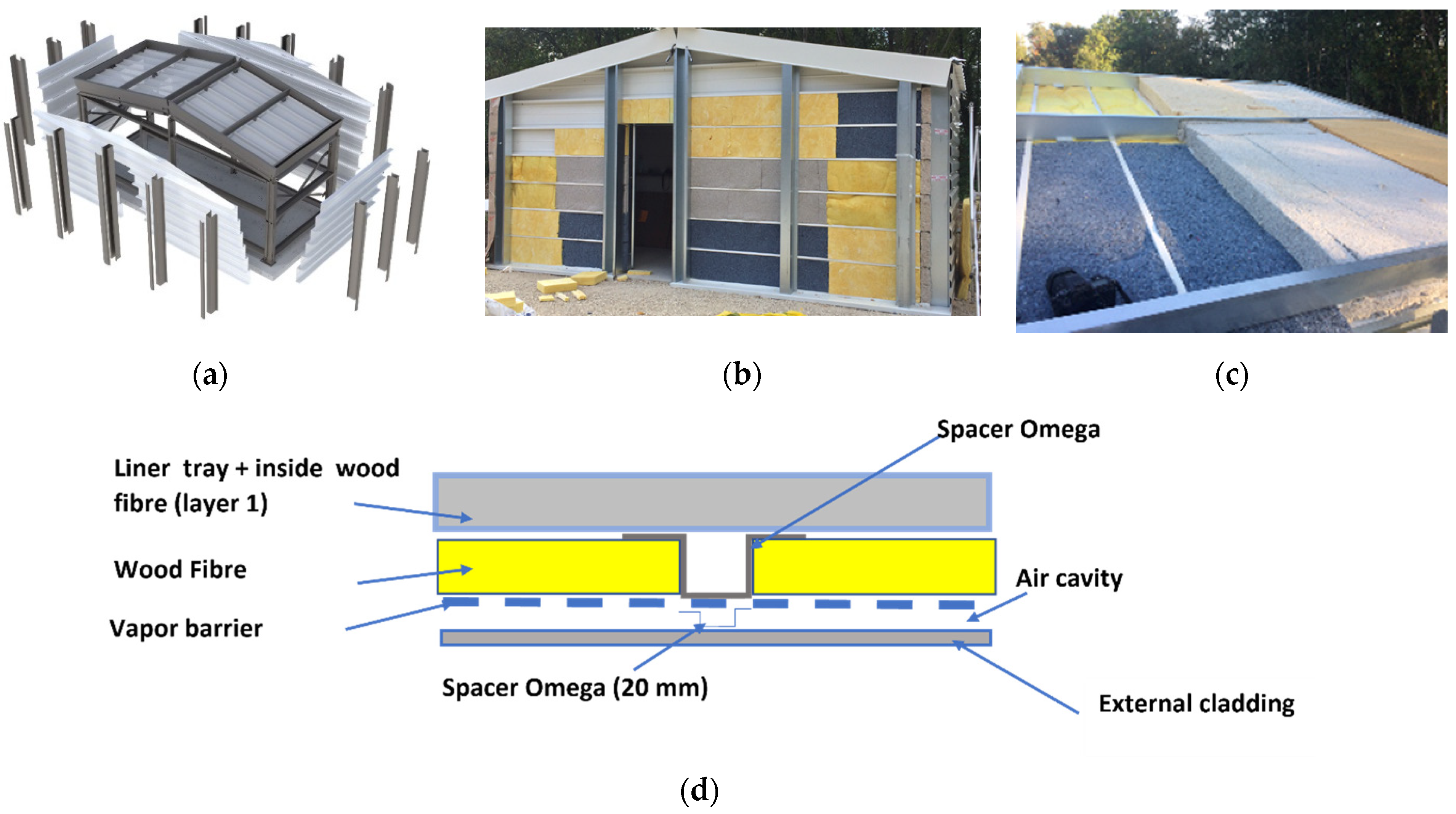
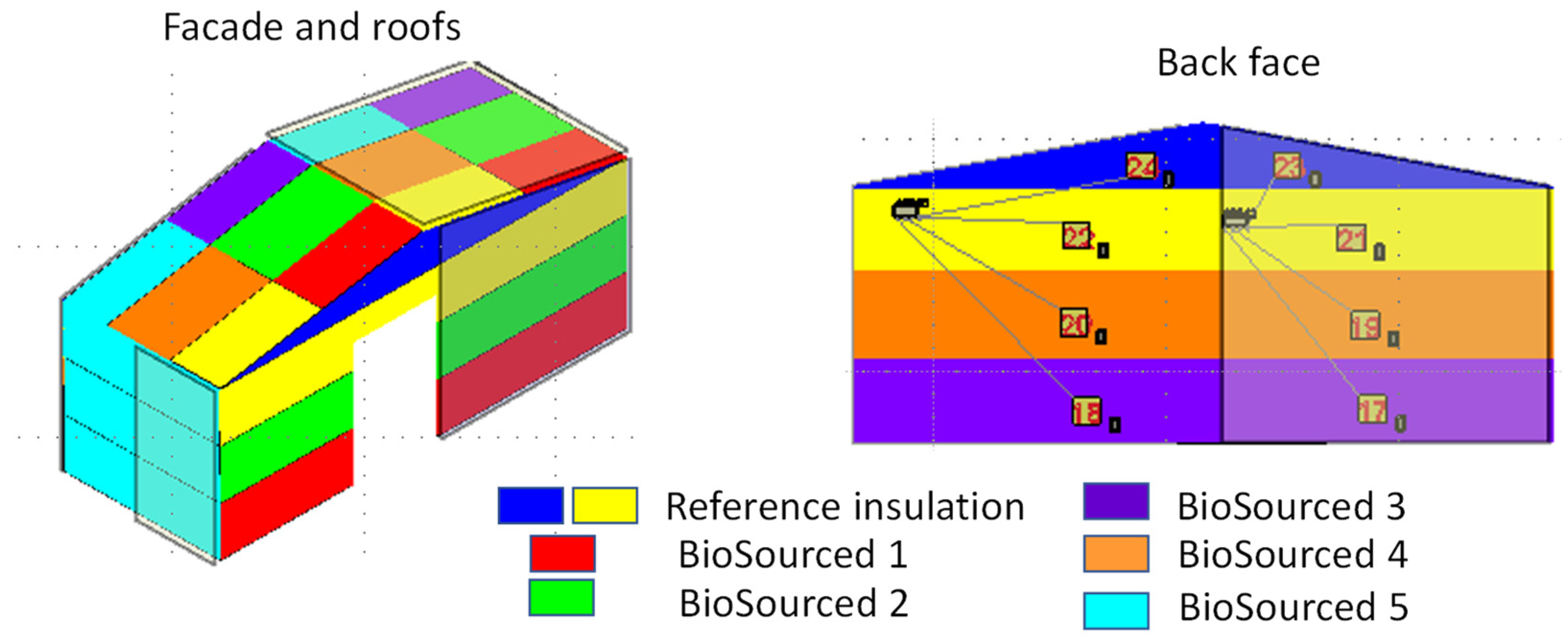
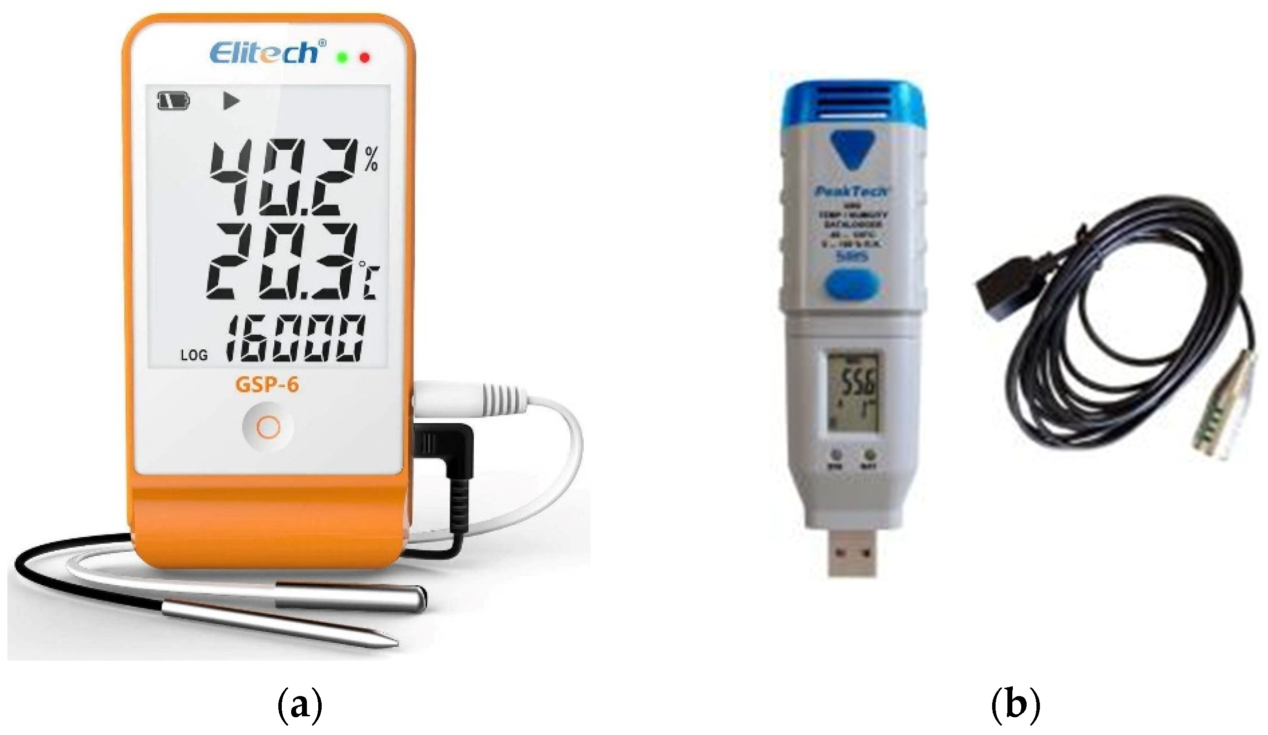
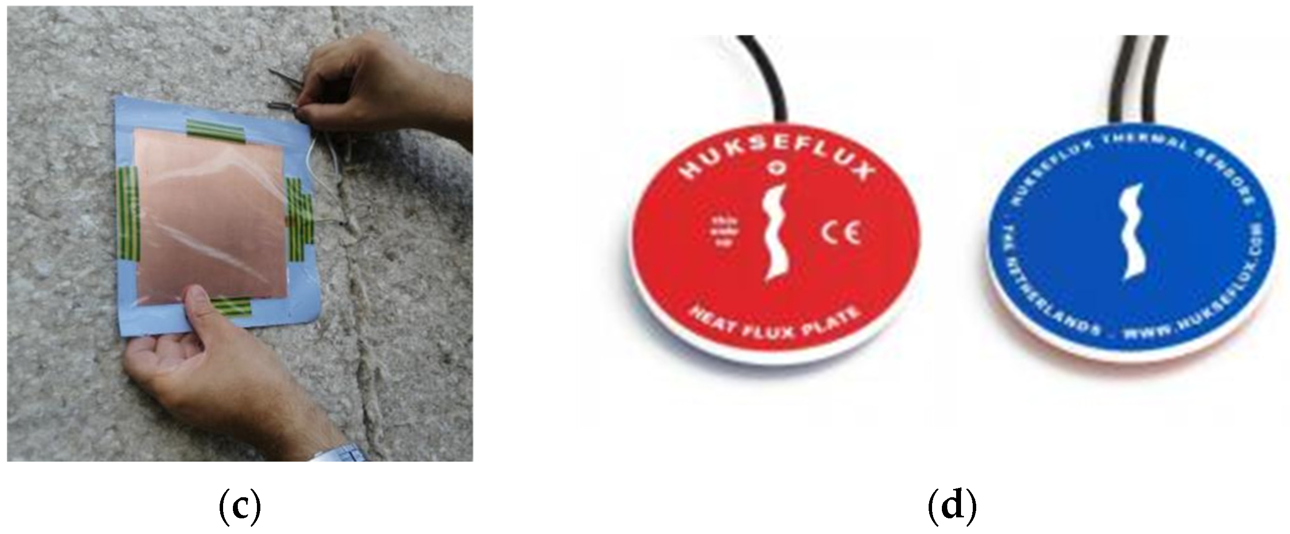
In this paper, firstly, the demonstrator building designed and constructed in the framework of the PROFEEL program [21,22] is described. The walls and the roofs of the demonstrator are made with panels of different insulating materials, including, on one hand, five bio-based insulating materials and, on the other hand, a classical mineral insulator, used as a bench material. Bio-based insulators used in the demonstrator are all manufactured by treating naturally derived components to form fibers, particularly, hemp, cellulose wadding, bio fibers, wood fibers and recycled textiles. A system for longtime, continuous monitoring and recording of temperature, relative humidity and thermal flux on each panel is designed and installed. The details of this measurement system follow the description of the demonstrator. Then, the analyses performed on recorded data for estimation of thermal resistance of each panel are presented along with associated theoretical and numerical models. Two alternative analyses are performed. Firstly, the normative analyses are performed following the ISO 9869-1:2014. This normative estimation is based on the Heat Flow Meter method (HFM) and so-called “averaged model” [23], which, when the conditions of use are respected, gives acceptable estimation of thermal resistance [24]. Secondly, a more rigorous numerical approach is used on the same data, making use of a parameter identification technique and an inverse analysis. A similar problem of thermal parameters identification from in-field data using coupled thermo-hygric modeling [24,25,26,27] was resolved in [19,28,29]. In the inverse analysis method proposed here, unlike a previous work by some of the authors in this paper, a semi-analytic method is used to solve the direct problem instead of the use of a finite difference software [29], estimated to be more time-consuming. The base for this semi-analytical method for the direct problem is the quadrupole model [9,24,28]. The principal contribution of the semi-analytical method proposed here resides in the adaptation of the quadrupole model for long, uncontrolled time-series data. The discussion of results and general conclusions close the paper.

2. Materials and Methods

2.1. In-Field Measurements and Data Recording

The demonstrator was designed and erected in the framework of the program PROFEEL [21] managed by the French Quality Construction Agency (AQC) in collaboration with the French Ministry of Sustainable Development. This program groups, among others, the producers of cold formed metal profiles for structures, envelopes and sandwich panels, members of the organization “Enveloppe Métallique du Bâtiment” [22] and French producers of bio-based insulators. The demonstrator was designed and equipped to answer the questions about the usability of existing bio-based insulation materials on steel-coated envelops, about the evolution of the efficiency of such systems with the variation of environmental conditions, in particular with the humidity variation, and finally about the durability and resistance of these systems to bio-agents such as fungus, insects or rodents.

2.1.1. Description of the Non-Structural Cold Formed Steel Envelope and Structural Portal Frame Constituting the Demonstrator

The cold formed structure (portal frames, rails, purlins and bracing system), the walls and pitched-roof double-skin system of the demonstrator building (Figure 1a–c) were purchased by Joris Ide Group. Arcelor Mittal Construction, France, carried out the assembly. The demonstrator is a typical double-skin steel building, designed following the normative rules for such type of buildings. The only difference of classical double-skin steel systems is that the walls and the pitched roof use panels of five bio-based insulating materials and panels from a bench mineral insulation (Figure 1d). In the clad, each wall consists of internal liner trays (height h = 400 mm; width w = 92 mm; thickness t = 0.75 mm), omega spacers (h = 180 mm, t = 1.5 mm), added omega spacer (h = 20 mm, t = 1.5 mm) and external horizontal profiled sheets conformed with European norm EN 14782 (t = 0.75 mm).
The role of omega spacers is to maintain a 20 mm air gap between the outer skin and the bio-based insulation layer, to ensure a natural ventilation. An acoustic system (perforated liner tray) is equipped in one of the gables. It is insulated with bench material panels and bio-based panels, some placed in contact direct with the perforation, and the other part using a vapor barrier between panels and outer cold formed steel sheet.
The roof is constituted by two non-ventilated double-skin systems: one with an in-side skin and a non-perforated liner tray (h = 400 mm; w = 92 mm; t = 0.75 mm) and the other using perforated inside profiled sheets (t = 0.63 mm). Both systems use insulating panels of bench insulator (mineral wool) and bio-based insulators. A vapor barrier is added on the up-right side of the pitched roof, between the insulating panels and outer skin. In all cases, omega spacers (h = 160 mm; t = 1.5 mm) and the classical external profiled sheet (length L = 1000 mm; w = 333 mm; t = 3 mm) and spacers (h = 45 mm; t = 0.63 mm) are used. A 35 µm organic coating was applied to all faces of the steel profiles in contact with the bio-based insulation, while a Z275 metallic coating was applied to spacers. The steel grade of the liner tray is S320 GD and for the other profiles, S280 GD. Steel fixing and stainless-steel fasteners (diameter 6.3 mm) are used.
Five bio-based insulation materials, including hemp, cellulose wadding, bio fibers, wood fibers and recycled textiles, all industrialized materials used in construction techniques, along with glass wool, fill the panels used in double-skin walls and the roof. Glass wool, a widely used mineral insulation in steel-clad buildings, is the benchmark for the comparative study. Two types of glass wool differing in density, representing the most common insulations used in the practice of steel buildings, are used in walls and in the roof.
The panels of the same wall or of the same pitched roof side are randomly distributed spatially, as reported in Figure 2.

2.1.2. Measurements and Recording System for Relative Humidity, Temperature and Thermal Flux Monitoring

The design of the measurements system is performed before the demonstrator construction with the objective to assure a sufficient time resolution, yet a continuous longtime monitoring and recording of physical parameters of interest. The sensors for temperature, relative humidity and thermal flux in the center of panels, are installed during the demonstrator construction (Figure 3), while those on the internal and external sheets of the envelope, immediately after construction.
All data are recorded at a rate of four entries per hour (but the selected devices can record data up to one entry per second if necessary). For each panel, the in-wall temperature and relative humidity probes are connected to a single autonomous data logger (Figure 3a), while the thermal heat flow is measured and recorded by a second couple probe-data logger. Note, that the thermal heat flowmeters are installed between two layers of insulators, inside each panel, avoiding any convective or radiation flux. The fluxmeters used in the roof panels are designed by CAPTEC® (Fareham, UK) (Figure 3c) with a sensitivity of at least 120 µV/W/m2, twice that of commercial HFP01 heat fluxmeters from Hukseflux® (Delft, The Netherlands) (Figure 3d), used for wall panels, with a sensitivity of 60 µV/W/m2.
All recorded data are time footprinted to ensure the traceability of data and a post-logging synchronization of all data.
In parallel with these in-wall data monitoring, specialized sensors were installed on the outside and the inside of each demonstrator face (Figure 3b) to record the air temperature and relative humidity on the surface of the walls and pitched roof.
All data loggers for the thermal flux are equipped with a DC tension recording device at a 5 µV resolution, so that the thermal flow is measured with a precision of 0.04 W/m2 for the CAPTEC® flowmeters (used in the roof), and a resolution of 0.07 W/m2 for Hukseflux® flowmeters (used in walls). The devices used for temperature measurements are certified with an absolute error smaller than 0.5 °C in the interval −30 °C to 60 °C, while relative humidity (RH) is measured from sensors with absolute error smaller than RH = 3%.

2.2. Methodology for Thermal Properties Estimation from In-field Data

2.2.1. Global Transmittance Value U of Insulant Panels Using Heat Flow Meter (HFM) Method ISO 9869-1:2014 Recommendations [19,30,31,32]

The method for thermal transmittance value estimation from in situ measurements recommended by norm ISO 9869-1:2014 is based on the theoretical model known in the domain of building physics as “average method” [19,20,23]. Supposing that the thermal flux crossing the wall, as well as the temperatures on two faces of the wall, are recorded in long synchronized data series, the average method gives the simplest way to estimate the thermal transmittance (or alternatively thermal resistance). Noting the ith record of temperatures measured on the outer face by T i , e x t , the inner face temperature by T i , i n t and the thermal flux φ i , the average method recommended in the ISO 9869-1:2014 standard calculates the transmittance factor U (in K−1 m−2 W) for an element using Equation (1), in which, the summation runs over all records of the chosen period:
U = i φ i i ( T i , e x t T i , i n t )
The thermal resistance is the inverse of the thermal transmittance, and in consequence, one could use for its estimation the inverse of Equation (1), i.e.,
R = i ( T i , e x t T i , i n t ) i φ i
If the flux used in these equations is not purely conductive (for example if it contains some contributions of convective or radiation heat exchange), the parameters estimated in such a way by the Heat Flowmeter method (HFM) should be considered as effective ones [33]. In this work, since the fluxmeters are installed inside the envelope, between two layers of insulant material of each panel, no radiative or convective flux is measured, so the estimated values are the true ones. The use of Equation (1) and/or Equation (2) should be done with precautions when the flux and the temperature difference of outer and inner wall faces inverse signs during the period considered in calculus. Since this inversion sign of flux is observed in our data, in Equations (1) and (2), we use the absolute value instead of signed values suggested in these equations. The use of the average method is sometimes known as absolute value technique [34]. Further, as suggested in [19,20,32], we use longer and longer time series records, up to a convergence of estimated values of U and R.

2.2.2. Thermal Properties Estimation as a Problem Identification Problem

Unlike the thermal properties of insulation materials guaranteed by manufacturers and certified by laboratory tests, the in situ thermal properties of the panels constituted by heterogenous layers of different materials and voids (see Figure 1d) could only be estimated using special techniques, adapted for parameter estimation from in-field recorded data analyses [20,28,29,35,36]. The estimation of thermal properties from recorded data belongs to the well-known parameter-identification class of problems, for which various solution strategies are elaborated [9,24]. In particular, thermal parameters identification is known to be an ill-posed problem [24]. Contrary to a direct problem, that calculates the response of a system for known material parameters and boundary conditions, the parameter-estimation problem estimates the unknown parameters of a system given the conditions of its use and its response. The general strategy to solve a parameter-estimation problem consists of using a numerical or analytical model to solve the direct problem for a fixed, arbitrary chosen, yet physical meaningful, set of vector parameters θ that should be identified. Let note by Y c a l ( θ ,   x , t ) , the response of the system calculated by the direct problem for the fixed vector of parameters θ . The response Y c a l ( θ ,   x , t ) is a vector that contains the calculated values for some physical variables (here, thermal flow) in all points of space and time when some measured values Y m e s ( x , t ) are known. The parameter identification could be seen as a minimization problem of an objective function, also called cost or, loss function, formulated as: find among all physically acceptable vector parameters θ , the one θ * that minimize the loss function i.e., find θ * in order to obtain F ( Y c a l ( θ * , x , t ) ,   Y m e s ( x , t ) ) m i n .
The cost function could be as simple as the “Euclidian distance” between measured and calculated data, as in the least squares method (LSM), i.e.,:
m i n   F ( Y c a l ( θ * , x , t ) ,   Y m e s ( x , t ) ) = m i n i , j ( Y c a l ( θ * , x i , t j ) Y m e s ( x i , t j ) ) 2
Equation (3) could be used for a very different kind of physical problem and quite general approaches of minimization could be used independently from the physical problem, which intervene only through direct problem response calculation Y c a l ( θ , x , t ) . In this paper, the invers problem is solved using a gradient descent method (Levenberg-Marquardt algorithm) implemented in lsqnonlin solver from Matlab® (The MathWorks, Natick, MA, USA).
The specific physical problem resolved in a particular study of the inverse problem, intervenes in the inversion process through the direct problem. Here, the direct problem is the coupled heat and moisture transfer through the building envelope (see Appendix A). Due to strong nonlinearity of coupled heat and moisture transfer equations, even for the 1D problem, there is no known analytical solution for arbitrary boundary conditions and usually a numerical method is used to get the solution of the direct problem [29]. In order to avoid time-consuming numerical methods, here we do not resolve a system of a coupled differential solution. The strategy that allows for this simplification is simply inspired by the observation that if one splits the time analyses in shorter time sequencies during which the relative humidity varies little (such as to be considered as almost constant), then the equations could be resolved for each time sequencies separately. In particular, the thermal problem could be resolved by considering thermal properties during that sequency in which there is little or no variation of hydric conditions. This approach drastically simplifies the problem, since in that case, only the heat problem with constant thermal properties over a chosen time-sequency should be solved. In consequence, however, this problem has to be resolved over all time-sequences resulting from the splitting of the original data. Here, the choice of the time-sequences over which the relative humidity is considered as (almost) constant and their length is indicated in each inverse analysis performed (see Section 3).
For a time-window, for which thermal properties could be considered as constants, the obtained linear heat diffusion problem, in the 1D plan wall, could be resolved using the (semi)analytical quadrupole model [28,35]. For a one-layer homogenous slab, and a pure thermal diffusion problem, the temperatures and thermal flux on two faces of the slab are related in the Laplace transform space by (see [9,20,28]):
[ Φ ˜ 1 T ˜ 1 ] = [ M ] [ Φ ˜ 2 T ˜ 2 ] = [ A B C D ] [ Φ ˜ 2 T ˜ 2 ]
For our application, the Φ ˜ i , T ˜ i ( i = 1 , 2 ) in Equation (4) are the Laplace transform flux and temperatures, respectively, on two faces of the considered part of the building envelope. The terms of the quadrupole matrix [M] are:
[ M ] = [ A B C D ] = [ c o s h ( R · b p ) s i n h ( R · b p ) / b p b p s i n h ( R · b p ) c o s h ( R · b p ) ]
In this last equation, R and b are the thermal resistance of the slab wall ( R = e / λ in [K m2 W−1]) and its thermal effusivity ( b = λ · ρ · C p in [W s1/2 m−2 K−1]), respectively, while p is the formal Laplace transform variable. From the quadrupole Equation (4), one could calculate any two quantities Φ ˜ i , T ˜ i ( i = 1 , 2 ) if two other ones are known. In particular, the Laplace transform flux could be expressed as a function of the only two Laplace transform temperatures in the two faces:
Φ ˜ 1 = D B T ˜ 1 1 B T ˜ 2
To use Equation (6), one needs to obtain Laplace transform signals of temperatures on two sides of the slab. In active measurements inversion practice in laboratory, these signals are controlled and imposed during the test [28]. Usually, during experiments in laboratory, a sinusoidal signal is imposed on experiments on one side of the wall and the other side temperature is kept constant. Under such conditions, the Laplace transform variables in Equation (6) are easily calculated analytically.
Unfortunately, in infield conditions, one could not control the temperatures in the outside surface of the envelope skin: the environmental conditions are those produced by the local weather. For uncontrolled, discrete measured data, to obtain a Laplace transformation of temperatures T ˜ i ( i = 1 , 2 ) in Equation (6), represents some difficulties. Due to natural evolution of the weather in the demonstrator place, the temperatures do not follow some analytical function, so no analytical Laplace transform could be performed. A z-transform of the original signal, with discrete long data series, is generally not recommended, and here an alternative strategy is adopted. Firstly, signals of temperatures on both sides of the wall are represented as sums of Fourier series terms. Generally, a small number of terms of such series is sufficient to accurately describe the variation of time-series data as those collected in our demonstrator. From our tests varying the number of terms for temperature presentation, we found that 30 terms are quite sufficient. Nevertheless, in order to minimize the loss of information during the transformation, we adopted a representation of the temperature signal using 52 terms of Fourier series. A truncation of modelized data in both extremities of series is systematically performed in order to avoid bord effects (see later Section 4.1).
Once the temperatures are represented as a sum of Fourier series, using the properties of Laplace transform, the Laplace transform temperatures T ˜ i ( i = 1 , 2 ) are calculated as a sum of Laplace transform terms of Fourier series. The Laplace transform flux Φ ˜ 1 could then be calculated using the Equation (6).
The final step, obtaining the thermal flux in the real space, is performed by an inverse Laplace transform of calculated Φ ˜ 1 . For inverse Laplace transform (ILT) from discrete numerical data, various algorithms could be used. Our choice, to use the so-called CME algorithm [37,38], is guided by its robustness, its performance and above all, from its capacity to produce a response with no shift. We are not going further with details of this algorithm; regarding features and details of this algorithm, the interested reader is invited to consult the two cited references as well as the others cited therein for a detailed description.
To avoid any confusion, it is worth underlining here, the fact that the model used here for the direct problem is different from well-known Pentaur or GullfibR models [34] or even gray box ARX approaches [35]. Implication of these differences are discussed further in Section 4.1 of this paper.

3. Results

The demonstrator setup dates back to 2020 and the monitoring process is ongoing. Various documents of the PROFEEL program report the data of the first-year monitoring of the demonstrator. The object of this study are the measurements obtained during the second observation period, which lasted from July 2021 to December 2021. The recorded data are available in Supplementary Material of this paper. All measuring stations provide comparable results, but this article only presents and discusses recorded measurements on the pitched roof. This choice, to limit our analyses on pitched roof panels only, has the advantage to avoid the dependency of results on the orientation of walls. In fact, environmental conditions on various faces of the building are dependent on their orientation. It is unlikely that the roof panels, despite the moderated pitching of the roof, are exposed in almost identical outside environmental conditions.

3.1. Raw Data Description and Illustration

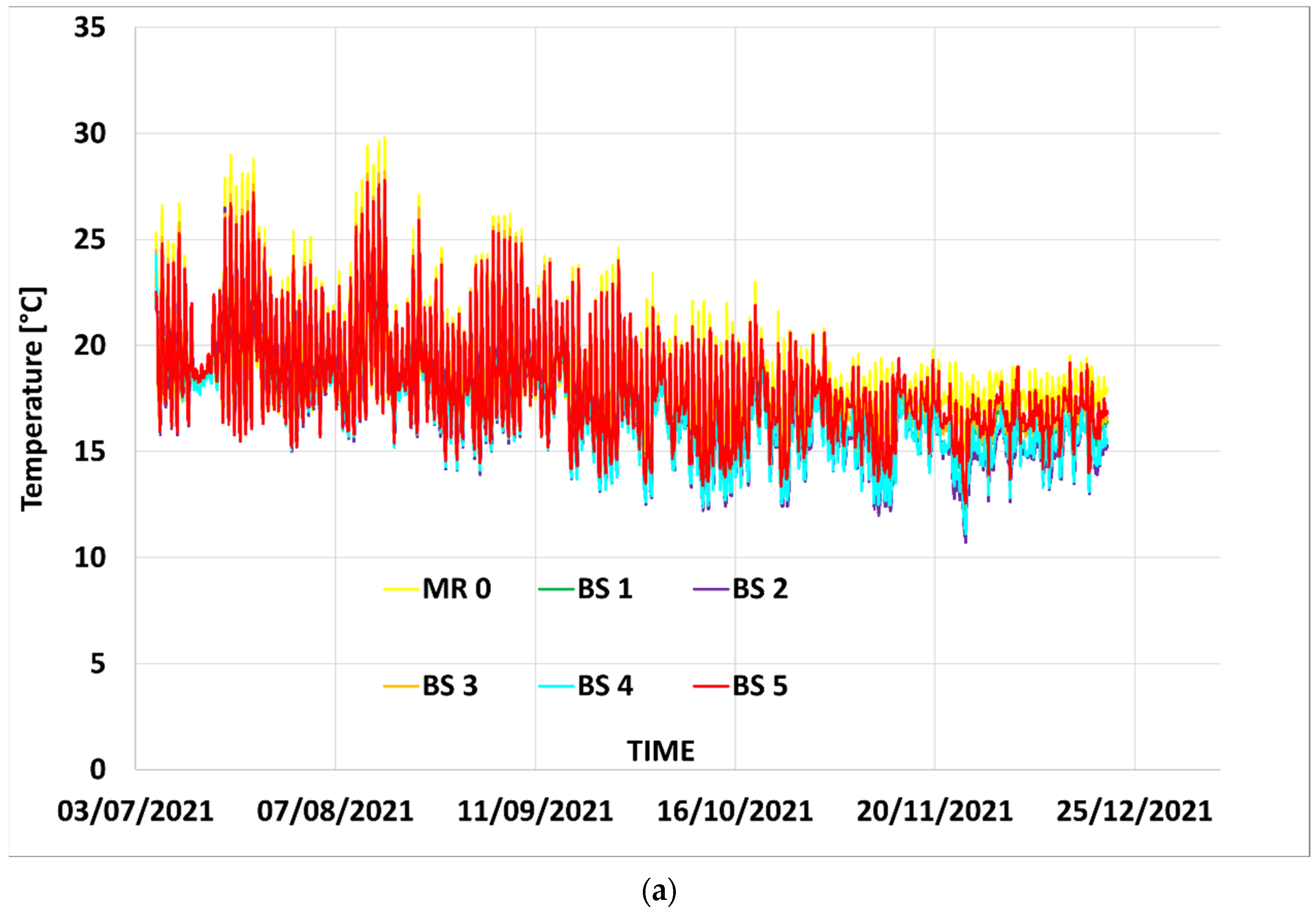
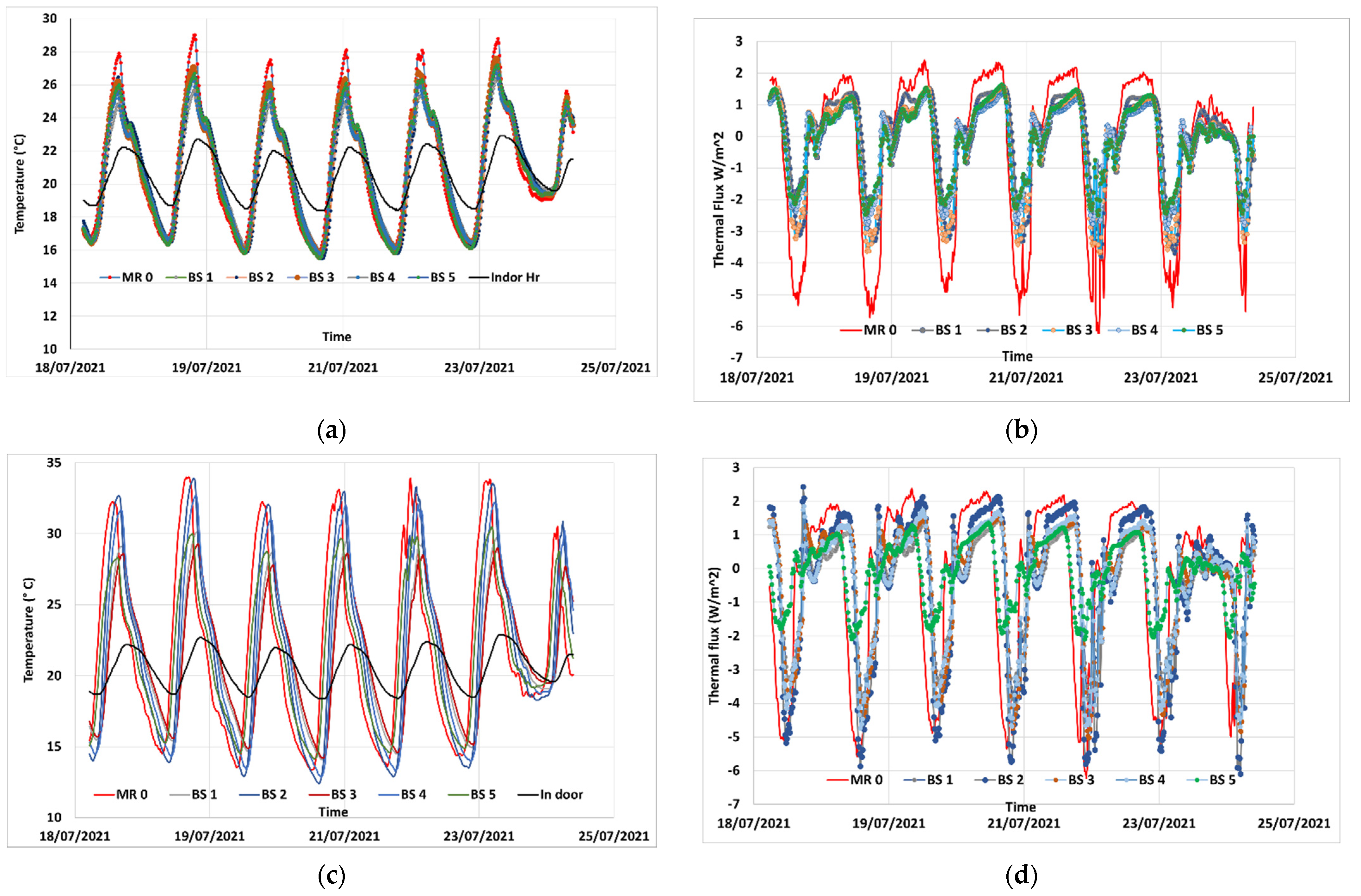
Figure 4a,b illustrates temperature measurements inside the panels of the roof, over the period of this study.
At this level of observation, the temperatures of all panels fluctuate similarly, achieving minimum and maximum values, on the same moments. Despite this similarity, one could observe that, some bio-based panels show systematically higher temperature values of all measured data, while some others show systematically, lower temperatures. This might indicate higher/lower thermal inertia of concerned insulators. Indeed, the temperatures on the center of panels, for the same conditions on the outer and inner skin of the envelope, depend on thermal conductivity, specific heat and density, all impacted by humidity and the amount of water vapor in the panels.
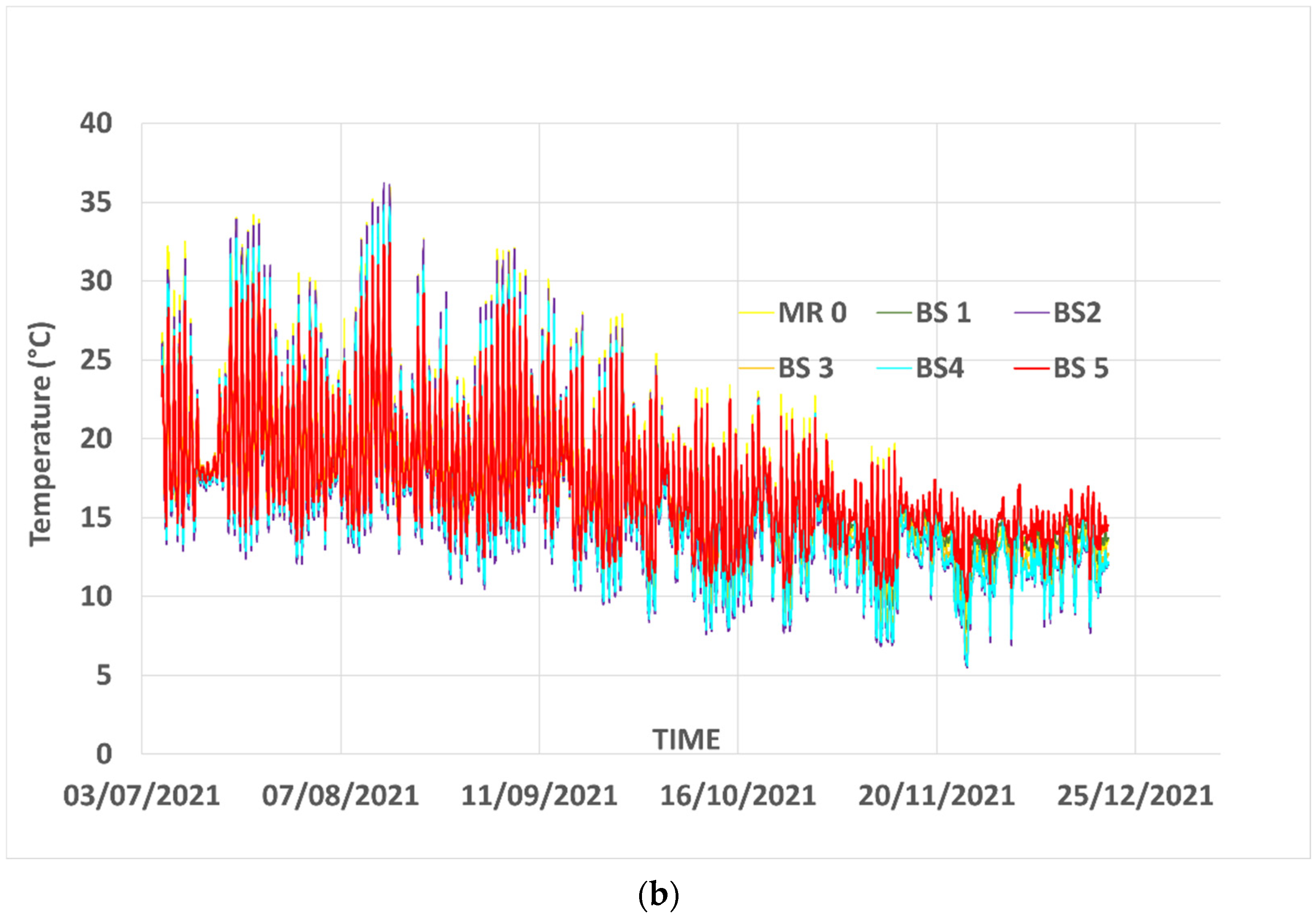
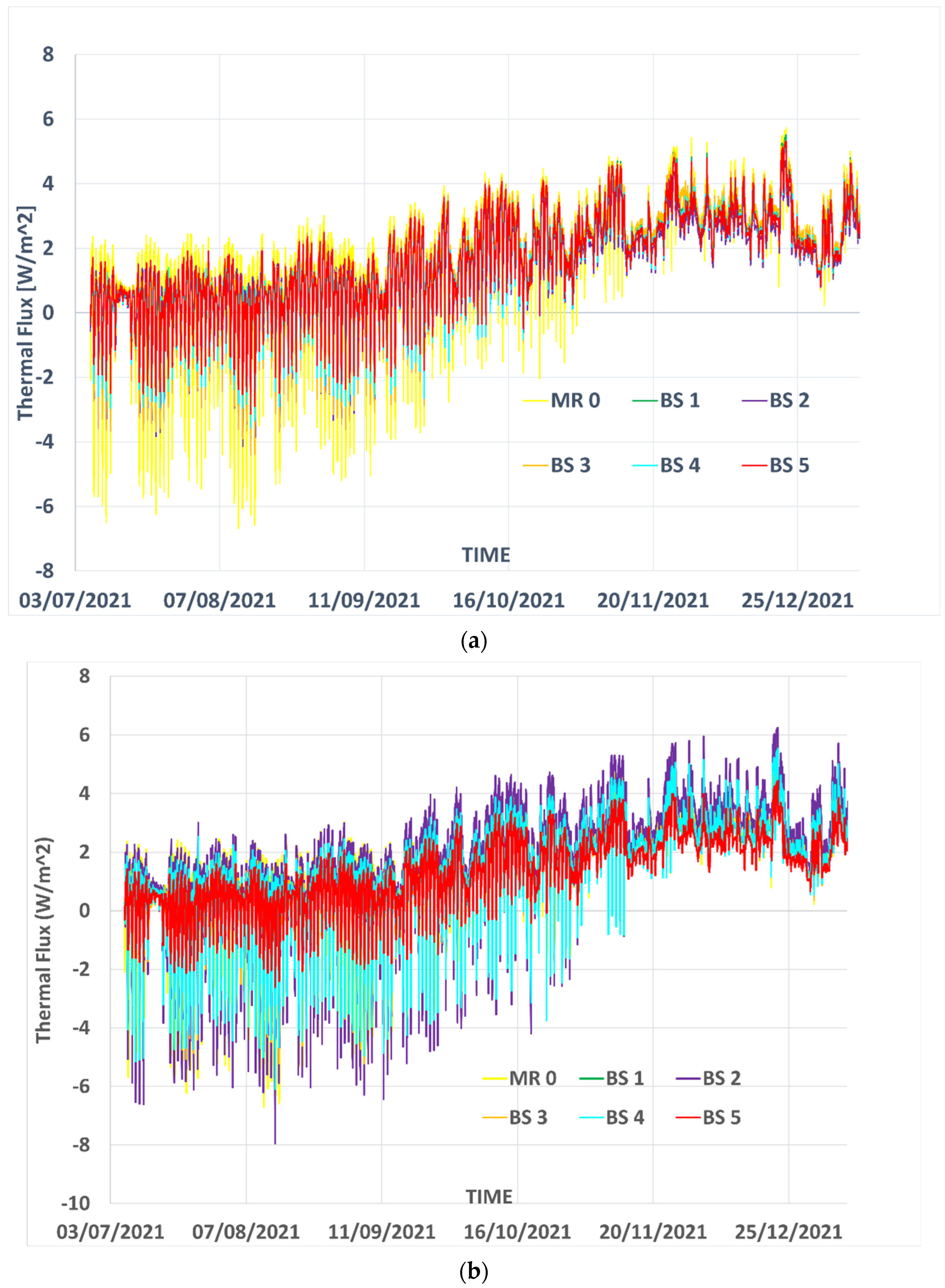
Figure 5a,b illustrates the evolution of moisture content in the panels as measured by probes situated in the center of each panel, between two insulation layers constituting each panel. One could easily distinguish in these graphics that the four last weeks of observations (from the end of November on), that coincide with the period of indoor heating, are characterized firstly by lowest values of relative humidity in each panel and, secondly, by a moderated amplitude of variations of humidity. The mineral insulant panels (MR0) manifest the highest amplitude of relative humidity variation during the summer and autumn season, independently of the presence or not of the vapor barrier, and one of the lowest values of relative humidity during the winter season.
It is important to point out that this variation of humidity could impact, at various extensions, the above-mentioned thermal characteristics (thermal conductivity and specific heat) that will also evolve with the relative humidity. For example, the thermal diffusivity being equal to the ratio of thermal conductivity (l) with the product of bulk mass and specific heat ( ρ · C p ), i.e., ( a = λ / ρ · C p ) its evolution with relative humidity could be non-monotonic, even if each of the physical parameters λ ,   ρ ,   C p of a porous medium are known to monotonically increase when the relative humidity increase. It is unlikely that the thermal effusivity (that to some extent better describes the thermal inertia) should increase monotonically when the relative humidity increases. One could expect that during winter seasons, when the relative humidity of the panel decreases, the thermal conductivity decreases too, leading to higher thermal resistance values. These remarks are recalled further in the discussion of results.
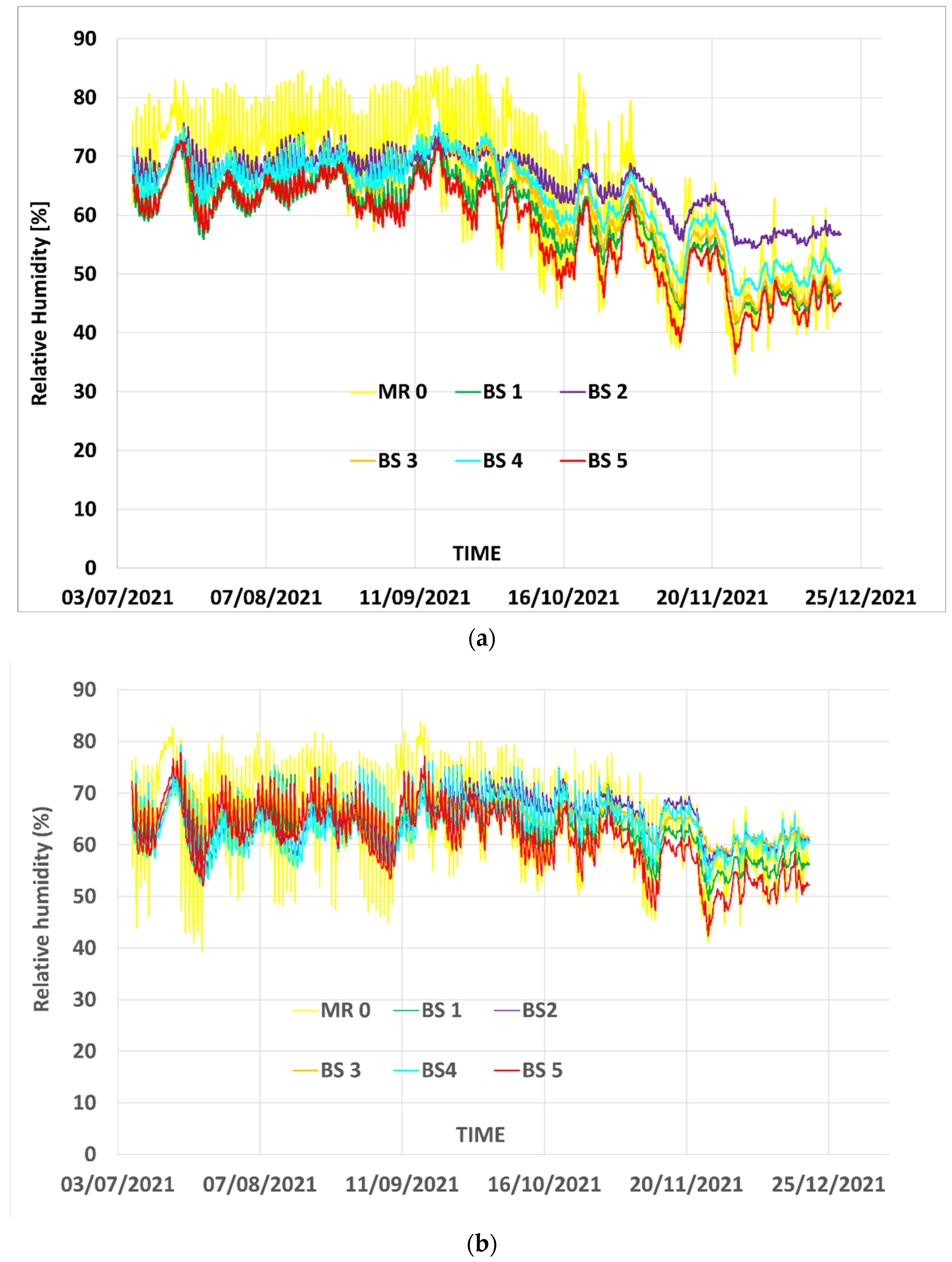
Figure 6a,b depicts the thermal flux on each roof panel during the considered period.
Since the variation of outdoor and indoor conditions (air temperature and humidity) are identical for all panels, the thermal flux measured in each bio-based panel could already be a good indicator of the thermal efficiency of each panel. Indeed, as long as the temperatures on the two sides of the panels are identical all the time, the measured thermal flux depends only on the state of the insulators and on its thermal properties.
The results of Figure 6a,b confirm that despite the different relative humidity differences previously depicted in Figure 5a,b, the thermal response of panels in terms of thermal flux is globally similar. More careful observations show that for both conditions, (with or without vapor barrier, respectively up-right and up-left sides of the pitched roof) some insulators, in particular the BS6, show remarkably lower in- or out-flow, while the bench insulator, in both conditions, has most often the highest values of the heat flow. Qualitatively, this is a strong indication of very good thermal insulation properties of the tested bio-based panels as compared to the mineral bench panels.
From data of up-right pitch roof panels, where a vapor barrier is used, one distinguishes that the in-flux in mineral reference panel is higher than in all other tested bio-based panels (Figure 6a). This is more visible during the summer and autumn, before the heating system of the building is turned on. One could speculate that this amplified response during summer and autumn could be explained by the differences in hygroscopic properties of insulations and strong thermo-hygric coupling mechanisms governing the process of vapor and heat diffusion in porous media.

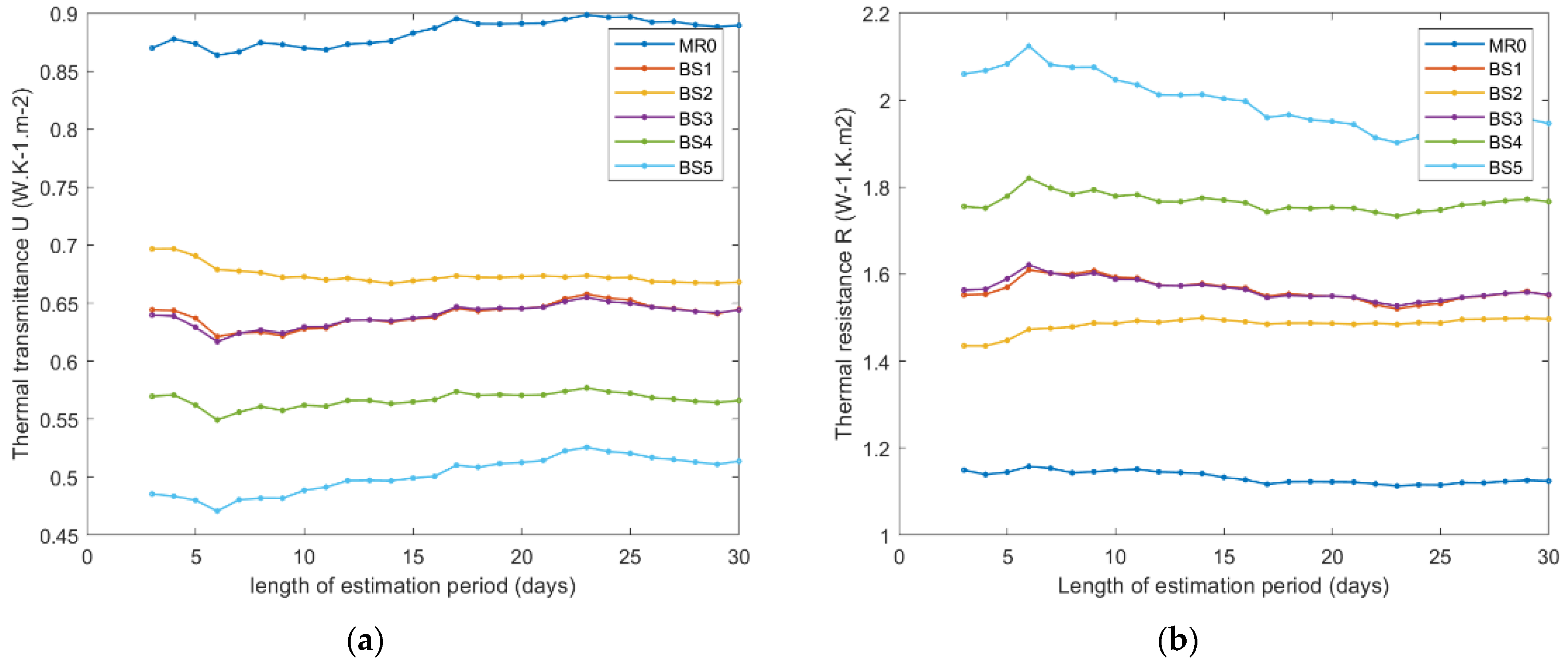
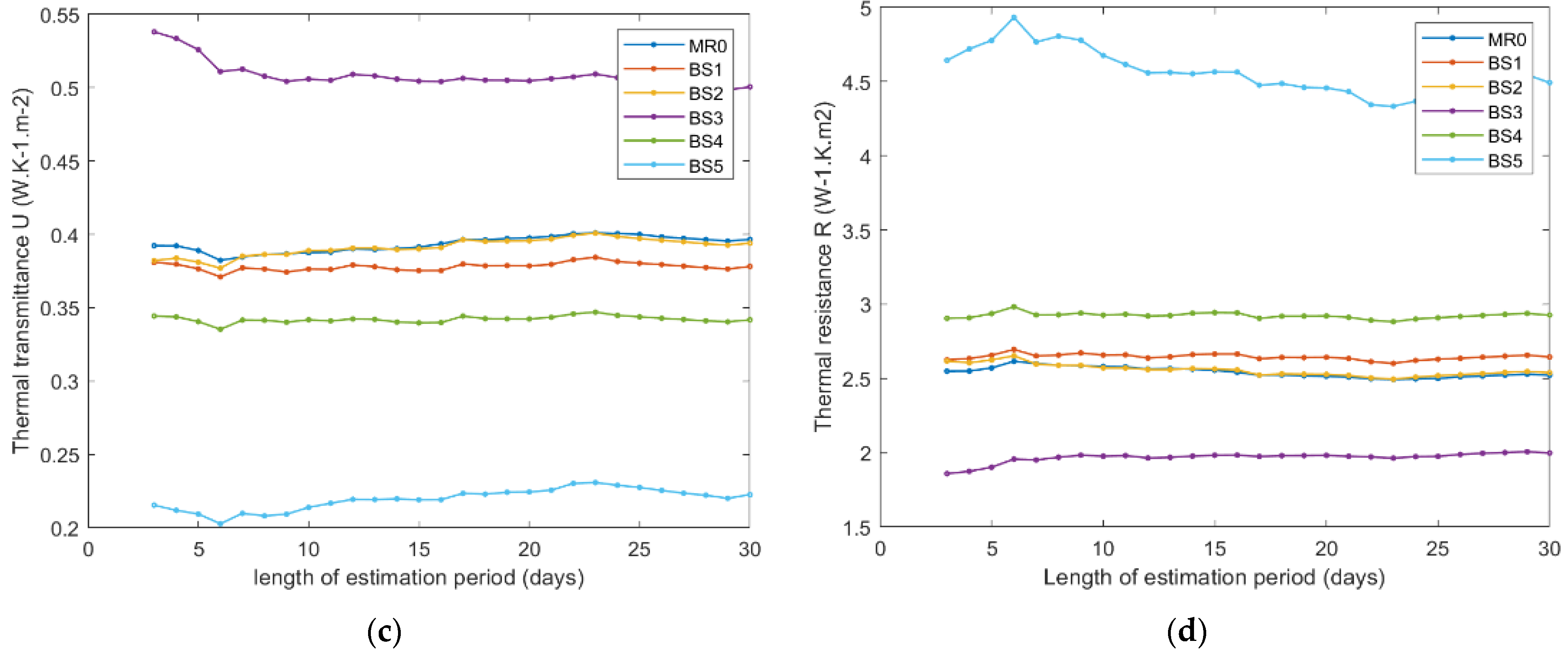
3.2. Estimated Thermal Transmittance Value U by HFM Method

As already discussed, the thermal properties, namely the thermal conductivity, is susceptible to evolve with moisture content in the insulators. For that reason, the thermal transmittance/resistance was estimated over two periods: firstly, during the first month of observation (summer season), where in-door heating and ventilation are off, and then during the last month (winter season) of observation when the heating system was on. We applied the methodology described in Section 2.2.1 in order to obtain the estimated values for each insulator panel, for various lengths of time series data (Figure 7a–d for the summer season, and Figure 8a–d for winter season). The thermal transmittance and thermal resistance, being the inverse of each other, the graphics of one of these quantities are sufficient. However, since in practice, some people are more friendly with one of these two parameters, both are presented in the figures, but the commentaries are limited to one of them.
The estimated values of transmittance/resistance and associated statistics are presented in the Table 1 and Table 2, respectively, for vapor barrier-protected insulator panels (right hand pitched roof) and without vapor barrier (left hand pitched roof panels).
The HFM method for estimation of thermal transmittance and thermal resistance, despite its simplicity in use, should be applied on a long time series in order to produce sufficiently accurate estimations [31,32,35]. However, for in-field measurements, the longtime observations are subject of environmental conditions variations, namely the variation of the air humidity (and consequently the insulators panel humidity), which in turn could trigger the evolution of thermal properties of the building component itself. Due to these variations of hydric conditions and eventually evolution of thermal properties as a consequence, the values in Table 1 and Table 2 should be considered as average estimators of nonconstant thermal properties over the observation periods.

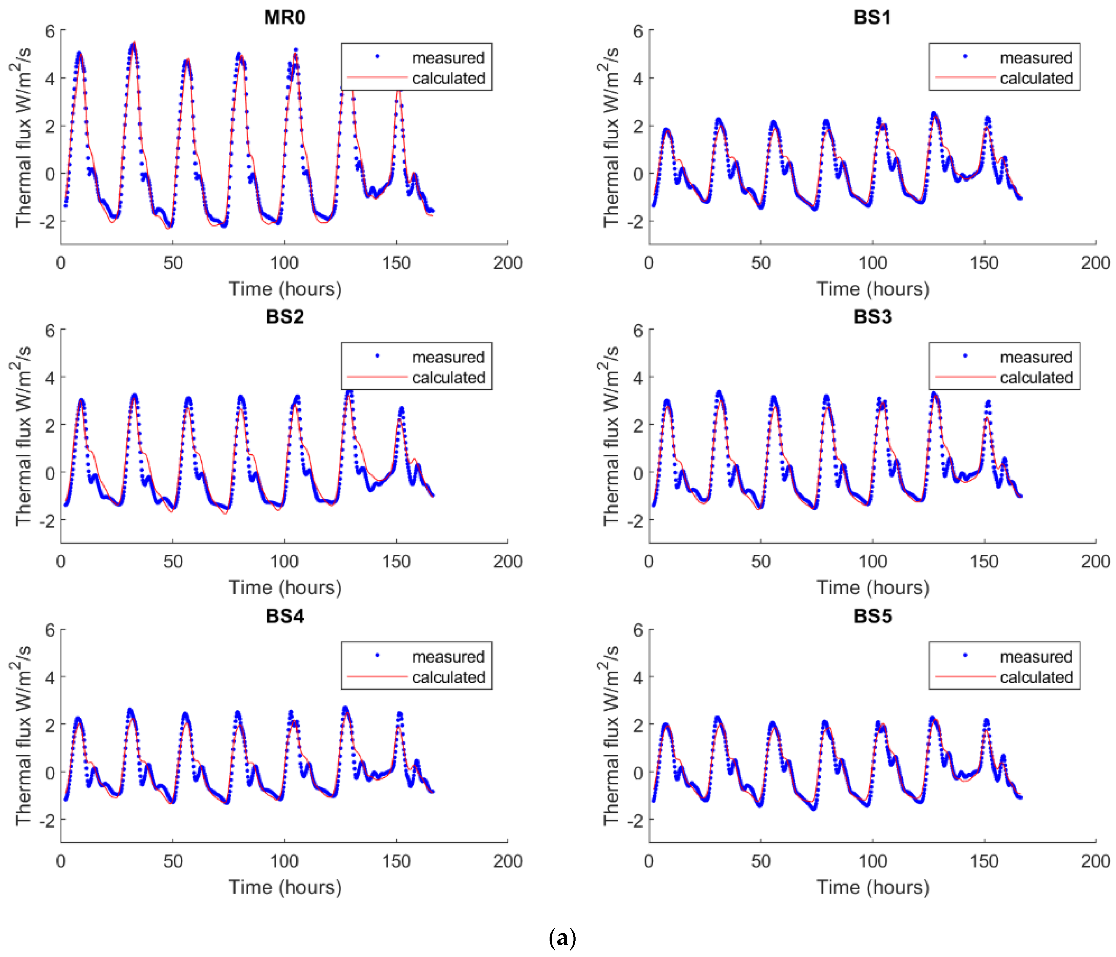
3.3. Estimated Thermal Resistance R and Thermal Effusivity from Inverse Analysis

In parallel with the HFM method, and in order to make a more accurate estimation of the thermal properties, the inversion procedure described in Section 2.2.2 is used here, to obtain, for each panel of the roof, the estimators of the thermal resistance and the associated effective effusivity. The first inversion analysis is performed over one week, chosen at the beginning of the observation period (heating system is off). Figure 9a,b shows the temperature records and measured thermal flux, used for the inversion process for the panels with vapor barrier. During this period, the humidity on various panels evolves between 40% and 80% for the panels without vapor barriers, and between 57% and 82% for the panels with vapor barriers.
Table 3 groups the results of estimated values of thermal resistance and effusivity of panels issued from the solution of the parameter-identification problem. The 95% confidence intervals bounds for estimated values of parameters are also given along with the MSE values, these last ones are an indicator of the quality of the inversion procedure.
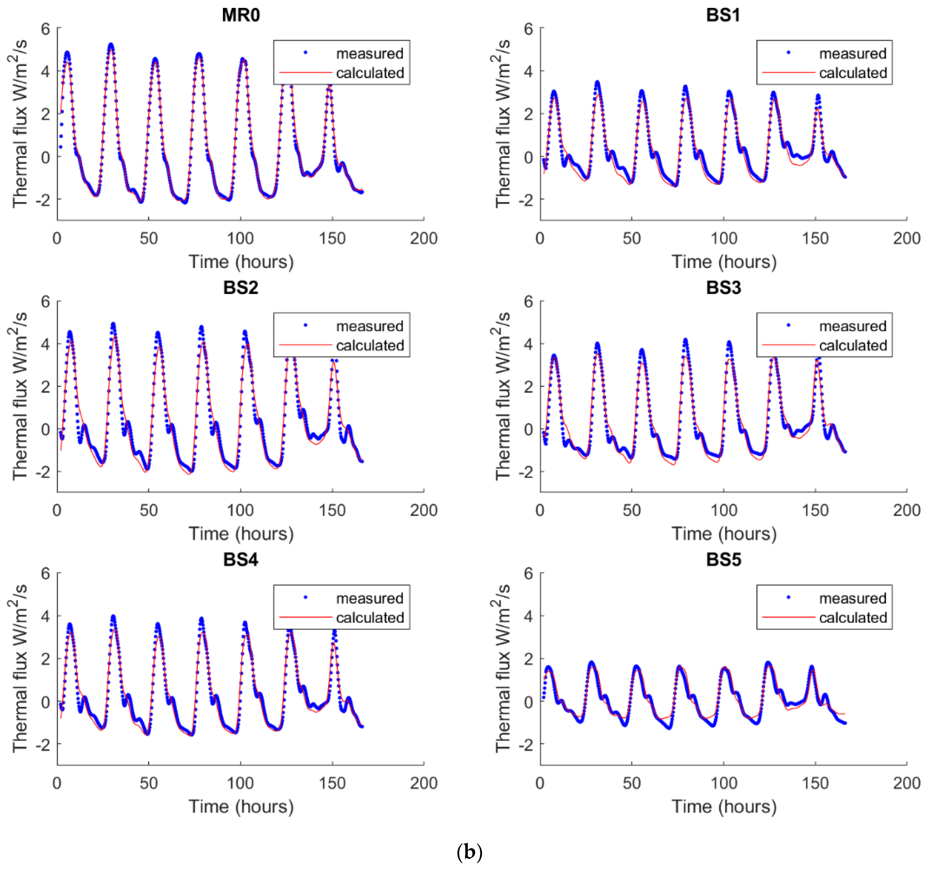
Figure 10 shows the predicted thermal flux, calculated using for the direct problem of the quadrupole model (Equation (6)) with identified thermal parameters (R and b) and measured thermal flux for each panel. A very good general accord is observed between measured and calculated data.
Using the same procedure and following the same objectives, the inversion is performed also for one week in the winter season when the heating system is on. Results of this inversion are indicated respectively in Table 4 and Figure 11a,b.

3.4. Assessment of the Risk for Water Condensation in Panels

The data for relative humidity variation in Figure 5a,b shows a high level of humidity during the summer and autumn season before the heating is turned on. While daily and seasonal variations of humidity in bio-based panels are clearly smaller than those of mineral-based panels, confirming their reputation as humidity regulators, the possibility of water condensation in the panels should be checked in order to avoid any consequence on human and structure health.
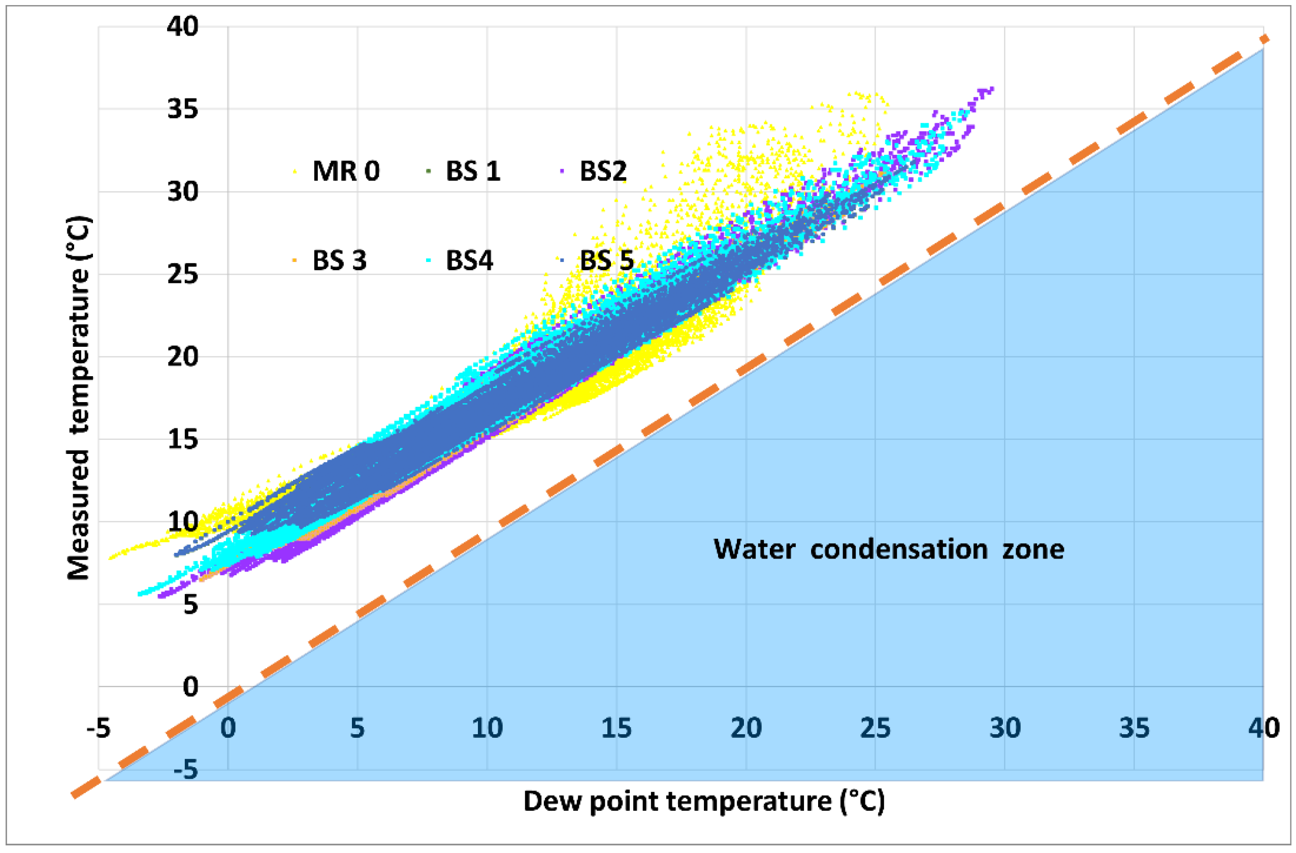
To assess the risk of water condensation in the panels, the dew point temperature is calculated and presented at any time and for each panel (Figure 12). In the center of insulations, the measured temperature is higher than the dew point temperature, indicating that there is no condensation risk in these points of the roof. However, these last findings should not be overinterpreted. They really confirm the impossibility of water condensation in the middle (half-thickness) of each insulating panel, but do not demonstrate the absolute impossibility of condensation everywhere on the roof. In fact, the measured points, considered for results presented in the Figure 12, are most likely, not the most vulnerable ones in respect to water condensation risk, at least, not all the time.

4. Discussion

The assessment of thermal properties of panels, their seasonal variations, as well as those of relative humidity on the center of panels, are strongly dependent on the quality of time series data collected by the measurements system and on the model used for these analyses. While some indications are already given on resolution and sensitivity of devices guarantying the quality of collected data (see Section 2.2), here we firstly discuss the choice of the approaches and models for infield thermal performances assessment of double-skin envelope with various types of insulant panels before responding to the questions formulated in the beginning of the paper.

4.1. On the Choice of Models and Approaches for Infield Thermal Properties Estimation of Double-Skin Steel Envelop

The normative model from the standard ISO 9869-1:2014 is based on the HFM method and in the form presented here is called the “average model without storage factor” [23,31,32,33]. This is a model, simple enough to be used in practice, yet robust and with acceptable accuracy for many engineering problems [31]. Equations (1) and (2) (without summation) are true for a steady state situation. The theoretical “average model” could be seen as an extension/adaptation of the steady-state equation by replacing the difference of the temperature and flux of steady state, with their respective mean values for the transient state problem [34]. This extension is based on assumption that in an infinitely long time series, the calculated mean values of temperature difference on the wall surfaces, on one hand, and the mean thermal flux, on the other hand, are almost in phase, i.e., the lag of time between the solicitation in the surface and thermal flux, in mean values vanished, because of the fact that the cumulated storage term becomes smaller as compared to the transmitted one. Since the time series used in infield measurements are always limited in time, the results provided by the HFM method and “average model” could only be considered as a quick estimation of the thermal transmittance (respectively, thermal resistance) of each insulator panel, that tends to the true values when the length of observed series tends to the infinity. For these finite (in time) estimations to be valid, a triple checking convergence of calculated values is required [31,32,35]: the length of the time series records should be superior of 3 days (for most of materials used in building construction); the variation of estimated values using measures over the last day U D and the before last day U D 1 varies less then 5%; and finally, the variation between estimated value U D and the values using only 2/3 of the observations U 2 / 3 D should also be less than 5%. All these conditions are satisfied in the case of data used in this paper, assuming one month time-series observation (Figure 8a–d and Figure 9a–d). Some authors that performed detailed comparison of various models used in the physics of buildings have estimated the error of this model to be up to 8%, when used in accordance with the above-mentioned constraints [20]. The use of this method without particular constraints (other than long series) would lead to errors up 12% [34]. These error estimations are obtained using a comparison with exact solutions, but there exists no theoretical tool to estimate the confidence bounds, which often is seen as an additional drawback of the average model [33].
The need for an alternative approach or thermal properties estimation, in the case of our application, is justified not only by these known concerns about the accuracy of the “average model”, but also by the fact that in long time series required for the use of this model, moderated variations of relative humidity (necessary to guaranty almost constant thermal properties) are not any more satisfied.
Different from a previous work from these authors, where a finite difference method was used to resolve the direct problem, here the quadrupole method is used. The finite difference method for solving the coupled equations of heat and moisture diffusion is not only a higher time-consuming method as compared with quadrupole method, but its use also requires hydric parameters (see Appendix A) to be known, which is not the case here. Besides that, in the problem treated here, we do not need the profiles of temperature distribution in every point along the envelope (that are furnished by the finite differences method): for the inverse problem, only the values of temperatures on two faces of the envelope are needed.
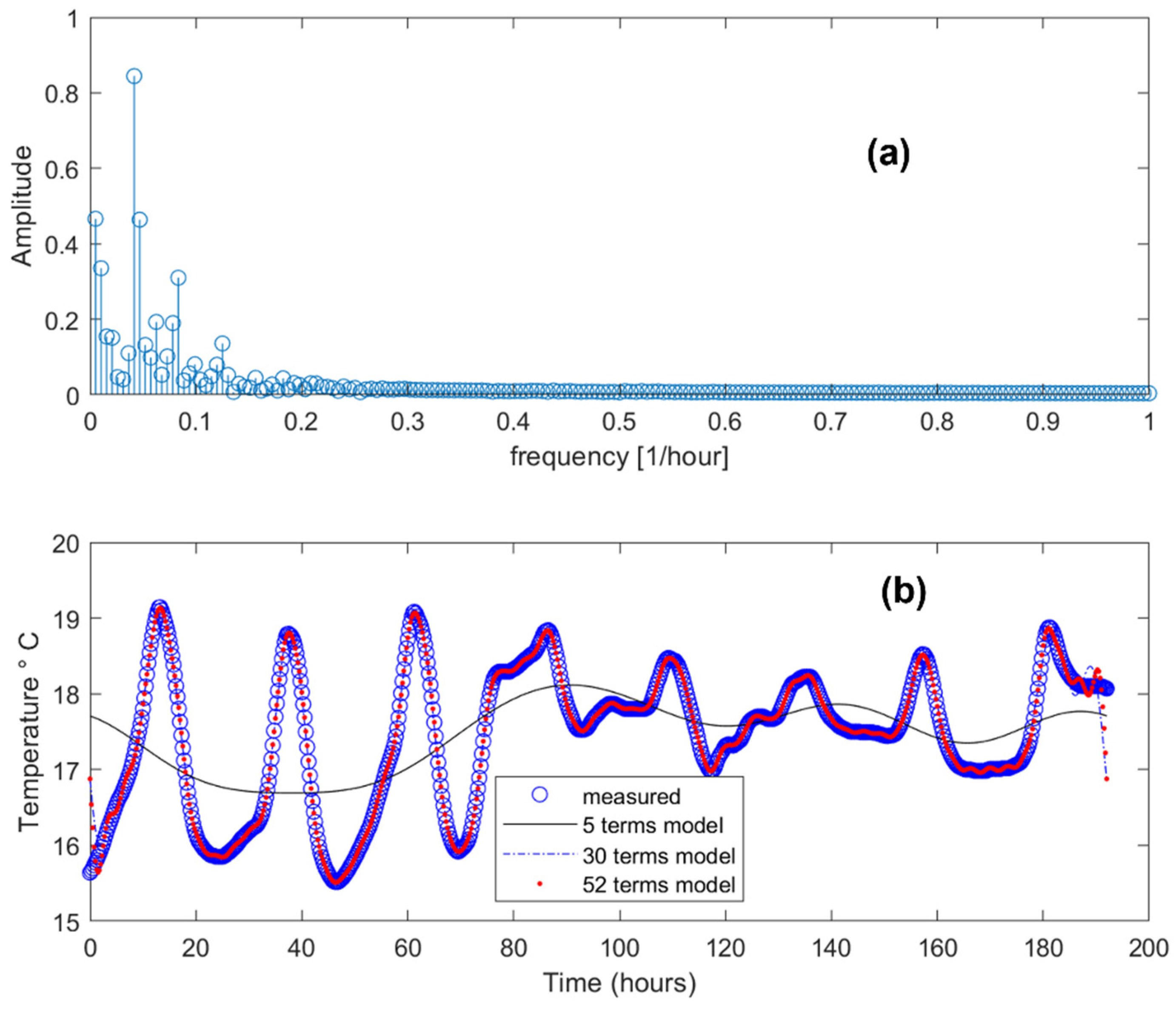
The quadrupole model used here to solve the direct heat diffusion problem is not a new model. What is new here is its use for the infield inversion data problem, i.e., for a transient problem with discrete data on uncontrolled boundary conditions. Despite the theoretical elegance of the model, its use in practice is conditioned by the capacity to easily calculate Laplace transform temperatures (see Equation (6)), and the inverse Laplace transform of flux calculated in the Laplace space. To overcome the first difficulty, the recorded temperatures on the inner and outer faces of the wall are firstly modeled using a sufficient number of Fourier series terms. The principle of the modeling of recorded temperatures using Fourier series, and the selection of the number of terms to be used in modeling, are illustrated by an example in Figure 13 (the data of the BS1 temperature sensor issued from graphic 9.a. are used for this example). The frequency-domain representation of data is presented in Figure 13a while Figure 13b represents the modeling of these data in time-domain using various numbers of terms of Fourier series. Even though there is no remarkable differences among models with 30 and 52 terms of Fourier series, in our analyses, 52 terms are used for modeling of input data.
The Pentaur and GullfibR models [23,31,34], the most used in dynamic thermal modeling of buildings, despite the similitudes, are different from the quadrupole model used here. Basically, the above-cited models use the fundamental solution of unit thermal charge in terms of Fourier series, to establish the transfer functions and obtain the flux response as function of temperatures on opposed surfaces of the envelope. The Pentaur model could be seen as an extension of the GullfibR model counting also for the information that one could have from the measured flux on the wall of both surfaces, if such data are accessible, and can be characterized as a statistical ARX model [23].
An alternative approach to resolve 1D, the direct diffusion problem, is to obtain the direct solution in the frequencies-domain [33]. The advantages to solve the problem on frequencies domain instead on time-domain, are discussed in [35]. However, as discussed in this same reference, despite the strong theoretical bases, the solution obtained needs to be adapted with some empirical transfer functions, to be useful in practice [33].
Whatever the strategy for direct problem solution may be, all solutions are affected by the initial distribution of temperatures in the wall which is, generally, unknown. The Pentaur and GullfibR models resolve this difficulty by defining an influence time tinf that precedes an instant of evaluation ti, such that all measured temperatures in interval [titinf; ti] should be included (multiplied by some coefficient to be defined) in the prediction of the thermal flux at instant ti, [20,23,38]. In this work, there is no way to introduce an influence time straightforward in predictions of direct problem, so the direct results, at the first instants of calculations are impacted from the initial distribution of temperature and these could be unrealistic to be compared with measured data. In order to overcome these errors, without any modification of the direct problem solution, we just ignore ncut first prediction results in the inverse analysis problem (Equation (3)), i.e., the minimization is not performed over all the data used for results prediction, but only on the free-from-initial-temperature-distribution results. As pointed out in [33], the initial state distribution affects the predictions only during a time of the same order as the characteristic diffusion time (depending on diffusivity and the thickness of the wall). For an expected thermal diffusivity k comprised in interval 10−8 m2 s−1 to 10−7 m2 s−1, and for the wall thickness e = 22 cm, the characteristic diffusion time (including a factor corrector as suggested in [39]) is estimated following Equation (7):
τ = e 2 π 2 · k ~ 0.22 2 π 2 · ( 10 8   t o   10 7   ) s   ~ ( 0.576   d a y s   t o   5.76   d a y s )
The estimation of Equation (7) gives the time after which, the predicted results are not any more affected by the initial distribution of temperature depending on the properties of the tested system. In analyses performed in this study, from posterior verifications of thermal properties, a length of 1.5 days was cut from predictions of the direct problem during the inverse problem procedure.
The low bound of characteristic diffusion time (Equation (7)) is a theoretical and practical justification of the sampling rate of recorded data (four samples/hour, or time sampling equal to 15 min). The sampling step-time of data is much inferior to the characteristic thermal diffusion and so, the sampling rate is quite sufficient for inverse thermal analyses performed here.

4.2. On the Performance of Bio-Based Panels Compared to Bench Panels

The results from the HFM method and parameter identification by inverse method are concordant and confirm the high thermal resistance of bio-based panels as compared to the mineral ones, justifying their suitability for use with a double-skin steel envelope. This confirmation is valid for all conditions of use of these panels (with or without vapor barrier).
It is useful to recall here that all analyses performed in this paper utilize the indoor temperatures and the recorded data (temperatures and thermal flux) inside panels (in half thickness of the wall). Due to the (approximately) symmetry of the envelope structure (see Figure 1d), one could estimate that the thermal properties of the outside half-thickness of the envelope are roughly the same as those of the half-inner thickness estimated in Table 1, Table 2, Table 3 and Table 4. The attention is drawn here in the fact that even in the case of perfect symmetry structure of two halves of thickness of the envelop, the thermal behavior/properties of the half-outside and half-inside are only approximately the same, because of the differences on their respective hydric states that are generally not identical.
The results in Table 1 and Table 2 show that the panels of bio-based insulants (BS1 to BS5), when no vapor barrier is used, have an overall thermal resistance comprised between 1.8 and 4.3 K W−1 m2, in the summer conditions and between 2.5 and 2.9 K W−1 m2 during the winter season. When the vapor barriers are used, these values are estimated between 1.6 and 2 K W−1 m2 during the summer season with very small variation from these values during the winter season. At the same time, the thermal resistance of the benchmark mineral panel without vapor barrier is estimated to be equal to 2.6 K W−1 m2 during the summer season and 2.4 K W−1 m2 during the winter season. Likewise, when a vapor barrier is used with the benchmark mineral insulator, the thermal resistance is estimated to be equal to 1.2 K W −1m2, with very small variation from one season to the other.
These values confirm that, from the point of view of thermal resistance, the constructive system, that makes use of bio-based insulators, is at least as better as the one that uses the mineral bench insulator (more often it is even better). In all monitored cases, except one (BS3 on unprotected conditions during the summer season), the bio-based insulators represent higher thermal resistance than the benchmark panels of mineral insulators.
These estimations are corroborated in all points by the inverse analyses (Table 3 and Table 4, Figure 10a,b and Figure 11a,b, for the summer and winter season, respectively). More rigorous than the HFM method, the parameter identification procedure from inverse analyses confirms the excellent thermal behavior of bio-based insulators used in this constructive system. Following results from the inverse analyses (Table 3 and Table 4), in all cases, the bio-based insulator panels have a thermal resistance either very close to that of the benchmark mineral insulator (MR0) or higher (sometime even much higher than MR0). A remarkable fact is that in all cases, the estimated values of thermal resistance from the HFM method are outside the 95% confidence bounds estimated by the inversion procedure, confirming the reserves of other authors in respect to the accuracy of the average method.

4.3. On the Hydric State in Insulants, Seasonal Variations of Humidity and Thermal Properties of Envelop

The dew point temperature analyses (Figure 12) show that there is no risk of water condensation in the panel. However, a more careful check of this point, namely by observations and measures, in other points of panels (and not only in their middle thickness) are necessary. Indeed, because of the gradient of the temperature and vapor pressure along the thickness of the insulating materials, other points on the building envelope could be more favorable to condensation than the middle of the panels. In particular, attention should be paid, and measurements should be performed on the interfaces between outside (inside) steel skin and the insulating materials, where the risk for water condensation could be higher. Although the recorded data are insufficient to quantify the evolution of moisture content in the panels and its impact on thermal properties evolution, some ideas, on the sensitivity of thermal properties of the bio-based insulators to the humidity fluctuation, could be given from inverse analyses results and comparison between winter/summer results. Indeed, it is shown that, during the winter season, once the heating system is on, the humidity in the panels decreases progressively and its fluctuations are almost invisibles (see the last weeks of measured data in Figure 5a,b, from the end of November). During this same time span, the thermal flux increased (Figure 6a,b). Of course, a port of flux increase during this period should be attributed to the increasing differences between in-room (heated) temperature and outside temperature as the winter season progresses. However, the inverse analyses (Table 4, Figure 12a,b) show that, at least, another part of the flux increase during the above-cited period should be attributed to the thermal resistance decrease: thermal resistance of all insulators has a decreasing tendance during the winter season, more pronounced for the panels used in conjunction with a vapor barrier. Otherwise, the estimated effusivity in the winter season is higher than in the summer season. This seems contradictory with the fact that all the factors intervening in the definition of effusivity ( b = λ · ρ · C p ) should decrease when the vapor content of the insulator decrease. This apparent contradiction between theoretical arguments and observation just demonstrates the role crucial of the air cavity in the walls (Figure 1d) and/or the role of the vapor barrier (when this barrier is used). While the thermal effusivity of the insulant itself should decrease during the winter period (or dry indoor air period), in the same period, the humidity of the outside air (and the cavity) increases, and so does the air cavity effusivity. This increment seems significant to compensate for the decrease in (dried) insulation, leading to an overall increase in the effusivity of the panels.

4.4. On the Role of Vapor Barrier on the Thermal Behavior of the Envelop

It is easy to see the role of the vapor barrier as regulator-of-humidity: in the panels equipped with the vapor barriers, this protection occupies a part of the air-cavity, replacing the air. This explains the double effect of the vapor-screen protection: firstly, due to its presence, the vapor barrier leads to higher thermal conductivity (lower thermal resistance); secondly, and this is the most significant role, due to its inner structure, the vapor barrier controls the circulation/conservation of the humidity on the insulant space. The presence of the vapor barrier modifies the retention curve of system vapor barrier–insulation on the upper values of the relative humidity (C zone absorption in the definition of [1]) making it possible that, finally, overall thermal properties of all insulants (benchmark mineral insulant MR0 and all the other tested bio-based insulators) varies very little, regardless the conditions (summer or winter).
The vapor barrier regulates the humidity (and makes uniform the thermal properties over seasons) by procuring a higher overall effusivity and a lower thermal resistance (see Table 3 and Table 4). This manifests with a more pronounced de-phasing thermal response of panels without vapor barrier compared to the evolution of the indoor temperature (Figure 10a,b, compared to Figure 9c,d). As it is shown theoretically by frequency-domain models [35], this dephasing is directly linked to thermal capacity, itself in our study impacted by the humidity evolution. The lag between the maximum (minimum) values of temperatures in the middle of each panel and the indoor temperature is almost the same for all vapor-protected panels (limited to about 30 min), while the most pronounced differences are observed in non-protected panels with a lag from 30 min to almost 2.5 h. Since there is no heating for the periods indicated in Figure 9a–d, the variation of the temperature in the panels is the consequence of outdoor temperature evolution (not presented and analyzed here), with the variations of indoor response as a final consequence. The higher the amplitude of the temperature variations and the faster these variations, the smaller the thermal inertia of the panel insulant. Certainly, the benchmark mineral insulators stand out as the one with the lowest thermal inertia (Figure 9c). For the panels with vapor barrier, wherein the variations of humidity are less important (regulated humidity), all insulants including the bench mineral insulator, have a similar response (same inertia in thermal response, Figure 9a) regardless of the season.

5. Conclusions

This study presented the work performed to measure and analyze the infield physical variables in the envelope of a demonstrator building, with the objective to check the usability of some bio-based insulants with the double-skin steel constructive system. For that, temperatures, relative humidity and thermal fluxes are recorded every 15 min in the center of five types of bio-based insulating panels as well as in mineral-based insulating panels, distributed in double-skin steel claddings and in the pitched roofs of the demonstrator building. The analyses and the comparative study are performed over data recorded from July 2021 to December 2021 on the roof panels only.
For all panels, the in-field thermal parameters estimations are performed by two methods: the HFM method following the ISO 9869-1:2014 standard in combination with the “average model” and a more complex and precise inverse thermal resistance and effusivity identification procedure. Both approaches lead to similar results, confirming that the thermal properties of bio-based insulant panels, as compared to those of classical mineral-based panels, are equivalent or even better, regardless of the seasonal conditions or the presence (or not) of vapor barriers. So, from the point of view of their thermal resistance, the use of such bio-based insulating panels in double-skin steel buildings is appropriate.
Confirming their regulators-of-humidity reputation, the bio-based insulating materials tested here manifest a higher hygric inertia as compared to the reference insulations. This higher hygric inertia leads toa better effective thermal performance when used with a vapor barrier in an acoustic solution (perforated profile/liner tray) in roofing. The measured data in the insulation indicates no risk of condensation on the measurement points.
The use of vapor barriers in that constructive system regulates the humidity as expected, ultimately procuring similar thermal properties of a given insulant whatever the environmental conditions and season may be. This is at least true in the range of the local environmental condition tested here. Unlikely, when vapor barriers are absent in the constructive system, a significant seasonal variation of thermal properties of all insulant panels is observed: when switching from summer to winter conditions, generally the thermal resistance increases and thermal effusivity decreases. The dephasing of temperatures on the panels in respect to air temperature variation outside, observed in panels without vapor barrier, is a direct indication of the role of the vapor barrier as regulator of thermal properties through its impact on humidity regulation.
The generalization of these conclusions and their confirmation call for analyses over all periods of observations (the observations are going on for two other years). The extension of these analyses on the wall panels will also elucidate the usability of these panels on the walls and the impact of wall orientations on their overall performances.

Supplementary Materials

The following supporting information can be downloaded at: https://www.mdpi.com/article/10.3390/su141710797/s1, The Excel file contain all recorded data from pitched panels.

Author Contributions

Conceptualization, D.H., D.I. and T.R.; methodology, D.H. and B.I.; software, D.H.; validation, D.I., T.R. and A.R.; investigation, D.H.; resources, T.R. and D.I.; data curation D.H. and B.I.; writing—original draft preparation, D.H. and A.R.; writing—review and editing, A.R. and D.H.; supervision, D.H.; project administration, D.H. and D.I. All authors have read and agreed to the published version of the manuscript.

Funding

This research received no external funding. The APC was funded by the Erasmus+ project KA2—Higher education strategic partnerships no. 2018-1-RO01-KA203-049214, “Rehabilitation of the Built Environment in the Context of Smart City and Sustainable Development Concepts for Knowledge Transfer and Lifelong Learning”—“RE-BUILT”.

Institutional Review Board Statement

Not applicable.

Informed Consent Statement

Not applicable.

Data Availability Statement

All data, scripts and results are available on request.

Conflicts of Interest

The authors declare no conflict of interest.

Appendix A

The mathematical equations describing the coupled transfer of heat and moisture in a porous media and taking into account the phase change, could be found on several references cited in this paper [1,14,30]. The principal equations are described here after, without describing all details leading to the final equations. Interested readers could find all these details in the above-cited references.
The equations of enthalpy and mass conservation are written respectively as [1,30]:
H T · T t = · ( λ T ) h e a t   f l o w + h v · ( δ p ( ϕ p s a t ) ) h e a t   s o u r c e
w ϕ · ϕ t = · ( D ϕ ϕ   l i q u i d   t r a n s f e r t + δ p ( ϕ p s a t ) v a p o r d i f f u s i o n )
In these equations, ϕ [ ] is the relative humidity (Hr), t [ s ] the time, T [ ° C ] the temperature, λ [ W · m 1 · K 1 ] thermal conductivity, P s a t   [ Pa ] the saturation vapor pressure, H [ J · mol 1 ] the total enthalpy, D ϕ [ m 2 · s 1 ] the liquid transfer coefficient, δ p [ ] the coefficient of vapor diffusion, h v   [ J · Kg 1 ] the evaporation enthalpy and w   [ ] the moisture content. In Equations (A1) and (A2), all properties could be the function of temperature and moisture content.
For the weak coupling or for the almost steady hygroscopic state, the second term of the right-hand equation could be neglected:
ρ C p · T t = · ( λ T ) h e a t   f l o w + h v · ( δ p ( ϕ p s a t ) ) h e a t   s o u r c e = 0
By considering the thermal conductivity constant within a fixed range of humidity, the right hand of equations simply represents the Laplacian operator, and the heat transfer equation becomes:
ρ C p · T t = λ Δ T
Unlike Equation (A1), Equation (A4) is linear and analytical solutions for simple configuration are available. In the particular case when the transfer problem could be considered 1D (this is the case, for example, of a plan wall with uniform thermal conditions in each face), Equation (A4) is further simplified to:
ρ C p · T t = λ 2 T x 2
A Laplace transform of Equation (A5) with appropriate boundary conditions leads to the quadrupole model [30]. Since, in reality, the conditions of constant moisture are not strictly met, very often the simplification consists of considering the thermal properties being a piecewise constant function of the moisture such that within a given range of humidity, one could use Equations (A4) and (A5).

References

  1. Korjenic, A.; Petránek, V.; Zach, J.; Hroudová, J. Development and performance evaluation of natural thermal-insulation materials composed of renewable resources. Energy Build. 2011, 43, 2518–2523. [Google Scholar] [CrossRef]
  2. Marjaba, G.E.; Chidiac, S.E. Sustainability and resiliency metrics for buildings—Critical review. Build. Environ. 2016, 101, 116–125. [Google Scholar] [CrossRef]
  3. Amziane, S.; Sonebi, M. Overview on Biobased Building Material Made with Plant Aggregate. RILEM Tech. Lett. 2016, 1, 31–38. [Google Scholar] [CrossRef]
  4. Bouasker, M.; NBelayachi, N.; DHoxha, D.; Al-Mukhtar, M. Physical Characterization of Natural Straw Fibers as Aggregates for Construction Materials Applications. Materials 2014, 7, 3034–3048. [Google Scholar] [CrossRef]
  5. Ed-Dariy, Y.; Lamdouar, N.; Cherradi, T.; Rotaru, A.; Barbu, M.; Mihai, P. The Influence of the Curing Conditions on the Behavior of Jute Fibers Reinforced Concrete Cylinders. Period. Polytech. Civ. Eng. 2021, 65, 1162–1173. [Google Scholar] [CrossRef]
  6. Islam, S.; Bhat, G. Environmentally-friendly thermal and acoustic insulation materials from recycled textiles. J. Environ. Manag. 2019, 251, 109536. [Google Scholar] [CrossRef]
  7. Pittau, F.; Iannaccone, G.; Lumia, G.; Habert, G. Towards a model for circular renovation of the existing building stock: A preliminary study on the potential for CO2 reduction of bio-based insulation materials. IOP Conf. Ser. Earth Environ. Sci. 2019, 323, 012176. [Google Scholar] [CrossRef]
  8. Schulte, M.; Lewandowski, I.; Pude, R.; Moll, L.; Völkering, G.; Kühn, U.; Kiesel, A.; Wagner, M. Environmental and Economic Performance of Bio-Based Insulation Materials: A Comparative Life Cycle Assessment. In Proceedings of the Miscanthus Conference “Bioökonomie—Aber Nicht Ohne Miscanthus”, Franzensbad, Czech Republic, 29–31 October 2019. [Google Scholar]
  9. Carslaw, H.S.; Jaeger, J.C. Conduction of Heat in Solids, 2nd ed.; Clarendon Pres: Oxford, UK, 1959. [Google Scholar]
  10. SCI. Steel Construction Institut. Available online: https://www.steel-sci.com/ (accessed on 12 July 2022).
  11. Pasanen, A.L.; Juutinen, T.; Jantunen, M.J.; Kalliokoski, P. Occurrence and moisture requirements of microbial growth in building materials. Int. Biodeterior. Biodegrad. 1992, 30, 273–283. [Google Scholar] [CrossRef]
  12. Viitanen, H.; Vinha, J.; Salminen, K.; Ojanen, T.; Peuhkuri, R.; Paajanen, L.; Lahdesmaki, K. Moisture and Bio-deterioration Risk of Building Materials and Structures. J. Build. Phys. 2010, 33, 201–224. [Google Scholar] [CrossRef]
  13. Jones, D.; Brischke, C. (Eds.) Protection of the bio-based material. In Performance of Bio-Based Building Materials; Woodhead Publishing: Sawston, UK, 2017; pp. 187–247. [Google Scholar]
  14. Maskell, D.; da Silva, C.F.; Mower, K.; Rana, C.; Dengel, A.; Ball, R.J.; Ansell, M.P.; Walker, P.J.; Shea, A. Properties of Bio-based Insulation Materials and Their Potential Impact on Indoor Air Quality. In Proceedings of the First International Conference on Bio-Based Building Materials, Clermont-Ferrand, France, 22–24 June 2015. [Google Scholar]
  15. Künzel, H.M. Simultaneous Heat and Moisture Transport in Building Components: One- and Two-Dimensional Calculation Using Simple Parameters; Fraunhofer IRB Verlag: Suttgart, Germany, 1995; ISBN 3-8167-4103-7. [Google Scholar]
  16. Zach, J.; Hroudová, J.; Brožovský, J.; Krejza, Z.; Gailius, E.A. Development of Thermal Insulating Materials on Natural Base for Thermal Insulation Systems. Procedia Eng. 2013, 57, 1288–1294. [Google Scholar] [CrossRef] [Green Version]
  17. Mouton, Y. (Ed.) Organic Materials for Sustainable Construction; Wiley & Sons Publishing House: London, UK, 2011. [Google Scholar]
  18. Rabbat, C.; Awad, S.; Villot, A.; Rollet, D.; Andres, Y. Sustainability of biomass-based insulation materials in buildings: Current status in France, end-of-life projections and energy recovery potentials. Renew. Sustain. Energy Rev. 2022, 156, 111962. [Google Scholar] [CrossRef]
  19. Choi, D.S.; Ko, M.J. Analysis of Convergence Characteristics of Average Method Regulated by ISO 9869-1 for Evaluating in Situ Thermal Resistance and Thermal Transmittance of Opaque Exterior Walls. Energies 2019, 12, 1989. [Google Scholar] [CrossRef]
  20. Larsen, S.F.; Hongn, M.; Castro, N.; González, S. Comparison of four in-situ methods for the determination of walls thermal resistance in free-running buildings with alternating heat flux in different seasons. Constr. Build. Mater. 2019, 224, 455–473. [Google Scholar] [CrossRef]
  21. Website of the PROFEEL Study Program. Available online: https://programmeprofeel.fr/ (accessed on 4 May 2022).
  22. Enveloppe Metallique. Available online: https://www.enveloppe-metallique.fr/ (accessed on 6 May 2022).
  23. Anderlind, G. Dynamic Thermal Models: Two Dynamic Models for Estimating Thermal Resistance and Heat Capacity from in Situ Measurements; Report A16; Swedish Council for Building Research: Stockholm, Sweden, 1996. [Google Scholar]
  24. Beck, J.V.; Blackwell, B.; Clair, C.R.S. Inverse Heat Conduction: Ill-Posed Problems; Wiley: Hoboken, NJ, USA, 1985. [Google Scholar]
  25. Duarte, R.; Flores-Colen, I.; de Brito, J.; Hawreen, A. Variability of in-situ testing in wall coating systems—Karsten tube and moisture meter techniques. J. Build. Eng. 2020, 27, 100998. [Google Scholar] [CrossRef]
  26. EN 15978:2011; Sustainability of Construction Works—Assessment of Environmental Performance of Buildings—Calculation Method. European Standards: Pilsen, Czech Republic, 2011.
  27. Tran Le, A.D.; Maalouf, C.; Mai, T.H.; Wurtz, E.; Collet, F. Transient hygrothermal behaviour of a hemp concrete building envelope. Energy Build. 2010, 42, 1797–1806. [Google Scholar] [CrossRef]
  28. François, A.; Ibos, L.; Meulemans, J. Estimation of the thermal resistance of a building wall with inverse techniques based on rapid active in situ measurements and white-box or ARX black-box models. Energy Build. 2020, 226, 110346. [Google Scholar] [CrossRef]
  29. Slaimia, M.; Belayachi, N.; Hoxha, D. In Situ Performance Assessment of a Bio-Sourced Insulation Material from an Inverse Analysis of Measurements on a Demonstrator Building. Adv. Eng. Forum 2017, 21, 460–467. [Google Scholar] [CrossRef]
  30. ISO 6946:2017; Building Components and Building Elements—Thermal Resistance and Thermal Transmittance—Calculation Methods. International Standards Organisation: Geneva, Switzerland, 2017.
  31. ISO 9869-1:2014; Thermal Insulation—Building Elements—In-Situ Measurement of Thermal Resistance and Thermal Transmittance, Part 1: Heat Flow Meter Method. International Standards Organisation: Geneva, Switzerland, 2014.
  32. Ficco, G.; Iannetta, F.; Ianniello, E.; Alfano, F.R.; Dell’Isola, M. U-value in situ measurement for energy diagnosis of existing buildings. Energy Build. 2015, 104, 108–121. [Google Scholar] [CrossRef]
  33. Courville, G.E.; Beck, J.V. Techniques for In Situ Determination of Thermal Resistance of Lightweight Board insulations. J. Heart Transf. 1989, 111, 274–280. [Google Scholar] [CrossRef]
  34. Lindfors, A.; Christoffersson, A.; Roberts, R.; Anderlind, G. Model based frequency domain estimation of thermal properties of building insulations. J. Therm. Insul. Bldg. Envs. 1995, 18, 229–260. [Google Scholar] [CrossRef]
  35. Shi, X.; Gong, G.; Peng, P.; Liu, Y. Investigation of a new kind of in-situ measurement method of thermal resistance of building envelope. Energy Build. 2022, 258, 111803. [Google Scholar] [CrossRef]
  36. Dowding, K.J.; Beck, J.V.; Blackwell, B.F. Estimating Temperature Dependent Thermal Properties. J. Thermophys. Heat Transf. 1999, 13, 328–336. [Google Scholar] [CrossRef]
  37. Abate, J.; Whitt, W. A Unified Framework for Numerically Inverting Laplace Transforms. INFORMS J. Comput. 2006, 18, 408–421. [Google Scholar] [CrossRef]
  38. Horváth, G.; Horváth, I.; Telek, M. High order concentrated matrix-exponential distributions. Stoch. Models 2019, 36, 176–192. [Google Scholar] [CrossRef]
  39. Aryasova, O.V.; Khazan, Y.M. Characteristic time of thermal and diffusion relaxation. Геофизический Журнал 2015, 37, 99–104. [Google Scholar] [CrossRef]
Figure 1. (a) Exploded view of demonstrator; (b) insulator setup between inner and outer steel profiled sheets; (c) view of the pitch roof in construction phase; (d) typical sketch of double-skin wall with an example of bio-based insulation panels layout.
Sustainability 14 10797 g001
Figure 2. Placement of insulating bio-based panels on different walls and pitch roofs of the demonstrator.
Sustainability 14 10797 g002
Figure 3. Devices used for the measurement system: (a) in-wall sensors for temperature and moisture content measurements; (b) on-wall (inner and outer) sensors for air temperature and humidity measurements; (c) CAPTEC® fluxmeters for in-wall thermal flux measurements; (d) HP01 fluxmeters for in-wall thermal flux on rear panels.
Sustainability 14 10797 g003aSustainability 14 10797 g003b
Figure 4. Temperatures recorded by in-wall sensors in the various panels: (a) the up-right roof panels; (b) up-left roof panels.
Sustainability 14 10797 g004aSustainability 14 10797 g004b
Figure 5. Relative humidity recorded by in-wall sensors in various panels: (a) the up-right side pitch roof panels; (b) the up-left side pitch roof panels.
Sustainability 14 10797 g005
Figure 6. Thermal flux recorded by in-wall fluxmeters in roof panels: (a) up-right side pitch roof panels; (b) up-left side pitch roof panels.
Sustainability 14 10797 g006
Figure 7. Estimated thermal transmittance/resistance for the summer season as a function of the length of observation period: (a,b) panels with vapor barrier panels; (c,d) panels without vapor barrier.
Sustainability 14 10797 g007aSustainability 14 10797 g007b
Figure 8. Estimated thermal transmittance/resistance for the winter season as a function of the length of observation period: (a,b) panels with vapor barrier panels; (c,d) panels without vapor barrier.
Sustainability 14 10797 g008
Figure 9. Input data for identification parameters problem during the summer season: (a,b) panels with vapor barriers; (c,d) panels without vapor barrier.
Sustainability 14 10797 g009
Figure 10. Measured and numerical predicted thermal flux during one week of the summer season using the identified thermal parameters: (a) panels with vapor barrier (up-right pitch roof); (b) panels without vapor barrier (up-left pitch roof).
Sustainability 14 10797 g010aSustainability 14 10797 g010b
Figure 11. (a) Measured and numerical predicted thermal flux during one week of the winter season using the identified thermal parameters in panels with vapor barrier (up-left pitch wall). (b) Measured and numerical predicted thermal flux during one week of the winter season using the identified thermal parameters in panels without vapor barrier.
Sustainability 14 10797 g011
Figure 12. Calculated dew point and measured temperature in the center of panels.
Sustainability 14 10797 g012
Figure 13. Example of treatment of input temperatures data: (a) frequencies presentation of temperature in BS1; (b) time-domain signal modeling with various number of Fourier series terms.
Sustainability 14 10797 g013
Table 1. Thermal transmittance and thermal resistance estimated using HFM and ISO 9869-1:2014 recommendations for panels equipped with a vapor barrier.
Insulator
Panel
Thermal Transmittance
(W K−1 m−2)
Thermal Resistance
(K W−1 m2)
MeanMaxMinStdMeanMaxMinStd
MR 00.8830.8980.8640.0111.1321.1581.1130.014Summer
season
BS 10.6400.6580.6210.0101.5631.6101.5200.025
BS 20.6740.6970.6670.0081.4841.4991.4350.017
BS 30.6390.6550.6170.0101.5651.6211.5270.024
BS 40.5660.5770.5490.0061.7661.8211.7330.019
BS 50.5020.5260.4710.0161.9942.1241.9020.063
MR 00.8710.8930.8420.0201.1481.1881.1200.027Winter
season
BS 10.7760.7970.7320.0141.2881.3651.2550.023
BS 20.5100.5230.4890.0081.9602.0431.9130.030
BS 30.7870.7980.7450.0131.2711.3421.2530.022
BS 40.5870.5920.5670.0051.7041.7631.6890.015
BS 50.7910.8130.7530.0141.2651.3281.2300.023
Table 2. Thermal transmittance and thermal resistance estimated using HFM and ISO 9869-1:2014 recommendations for panel without a vapor barrier.
Insulator
Panel
Thermal Transmittance
(W K−1 m−2)
Thermal Resistance
(K W−1 m2)
MeanMaxMinStdMeanMaxMinStd
MR 00.3930.4010.3820.0052.5422.6162.4940.04Summer
season
BS 10.3780.3840.3710.0032.6452.6952.6020.02
BS 20.3910.4010.3770.0062.5562.6532.4950.04
BS 30.5080.5380.4980.0091.9682.0061.8590.03
BS 40.3420.3470.3350.0022.9242.9832.8820.02
BS 50.2190.2310.2030.0074.5614.9324.3330.15
MR 00.4320.4350.4250.0032.3132.3562.2980.02Winter
season
BS 10.4070.4090.4020.0022.4562.4862.4430.01
BS 20.4020.4070.3970.0032.4852.5202.4580.02
BS 30.3570.3610.3490.0022.8002.8642.7730.02
BS 40.3400.3430.3390.0012.9382.9502.9170.01
BS 50.3990.4060.3950.0022.5052.5312.4650.02
Table 3. Estimation of thermal resistance and effusivity of insulator panels for the summer season using the parameter identification inverse problem.
Insulator
Panel
Thermal Resistance
(K W−1 m2)
Effusivity
(W K−1 m−2 s1/2)
MSE of Fitting
Estimated95% Lower Bound95% Upper BoundEstimated95% Lower Bound95% Upper Bound
MR 01.1941.1751.21348.12945.48850.7710.182Panels with vapor barrier
BS 11.7821.7301.83438.06535.90240.2270.117
BS 21.6471.5941.70047.42145.05149.790.242
BS 31.6421.6041.68026.50123.18429.8180.145
BS 42.0321.9672.09735.62433.63337.6140.128
BS 52.2942.2392.34930.70929.21632.2020.078
MR 02.8162.7922.84130.35729.74430.970.049Panels without vapor barrier
BS 13.5063.4313.58130.67229.92331.4220.117
BS 22.7132.6612.76613.82411.13916.510.234
BS 32.7922.7112.87251.25950.36752.1510.135
BS 43.1513.0723.22934.25733.37835.1360.107
BS 57.0886.8037.37319.83619.28620.3870.064
Table 4. Estimation of thermal resistance and effusivity of insulator panels for the winter season using the parameter identification inverse problem.
Insulator
Panel
Thermal Resistance
(K W−1 m2)
Effusivity
(W K−1 m−2 s1/2)
MSE of Fitting
Estimated95% Lower Bound95% Upper BoundEstimated95% Lower Bound95% Upper Bound
MR 00.9400.9330.94661.08255.1667.0040.070Panels with vapor barrier
BS 11.3631.3541.37292.49789.69295.3020.074
BS 21.9531.9431.96477.76375.94179.5860.038
BS 31.3031.2971.31084.89582.5287.2710.040
BS 41.7151.7061.72376.26974.51878.0200.035
BS 51.2801.2691.29153.6448.44258.8390.108
MR 02.3392.3252.35331.80529.84833.7630.057Panels without vapor barrier
BS 12.9452.9292.96247.77146.78748.7540.046
BS 22.5102.4942.52630.90628.60333.2090.086
BS 32.7802.7682.79363.82563.05864.5920.029
BS 42.4752.4612.48952.19950.89953.5000.046
BS 52.5362.5172.55514.14410.15018.1380.059
Publisher’s Note: MDPI stays neutral with regard to jurisdictional claims in published maps and institutional affiliations.

