

Time History Analyses of a Masonry Structure for a Sustainable Technical Assessment According to Romanian Design Codes


Abstract
:1. Introduction
2. Materials and Methods
- -
- seismic risk class Rs I, if R3 < 35%;
- -
- seismic risk class Rs II, if 35% ≤ R3 < 65%;
- -
- seismic risk class Rs III, if 65% ≤ R3 < 90%;
- -
- seismic risk class Rs IV, if R3 ≥ 90% [22].
3. Modeling of the Structure
3.1. Finite Element Model Description
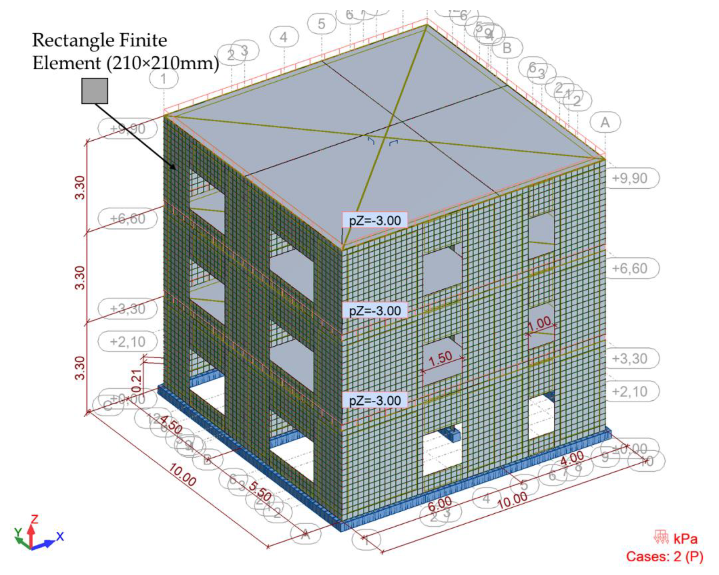
3.1.1. 2D Shells Linear Modeling
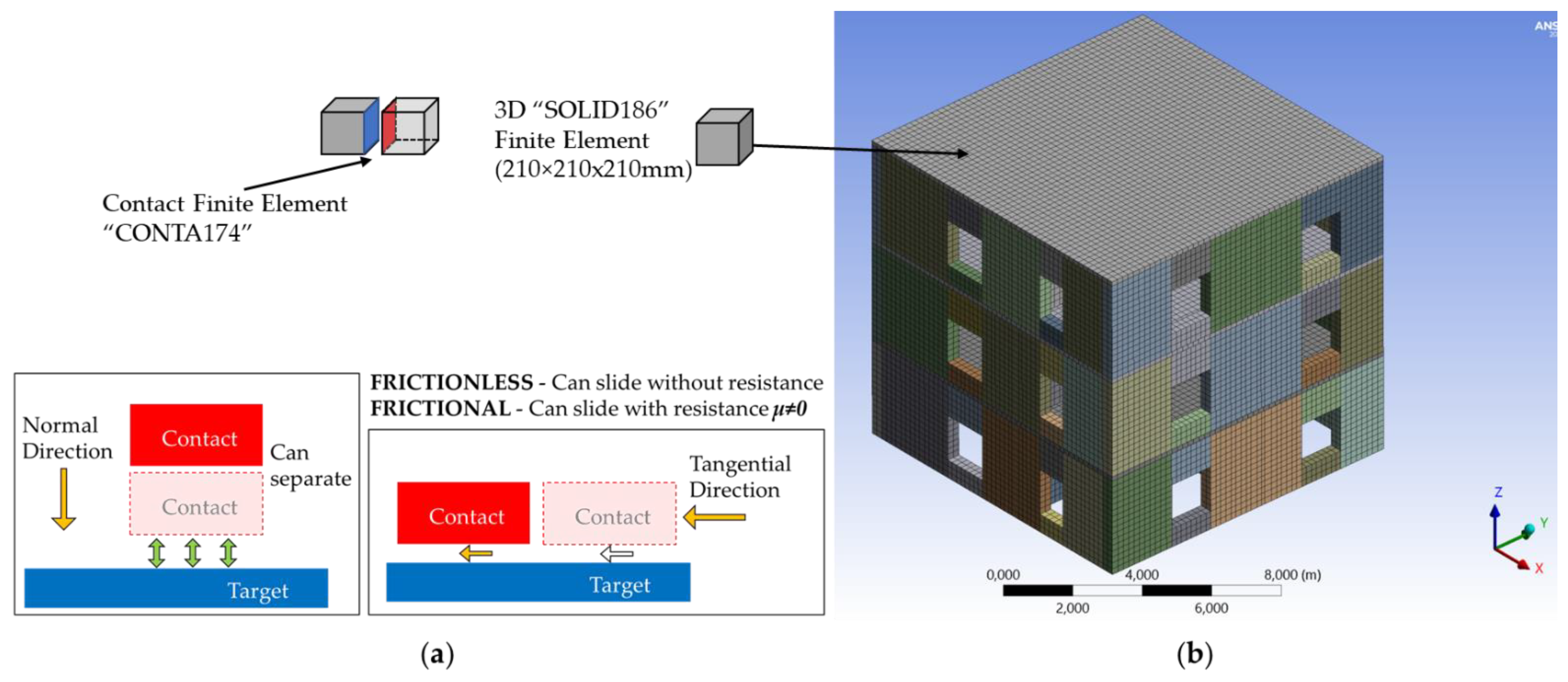
3.1.2. 3D solid non-linear modeling
3.2. Finite Element Loads Description
4. Results and Discussion
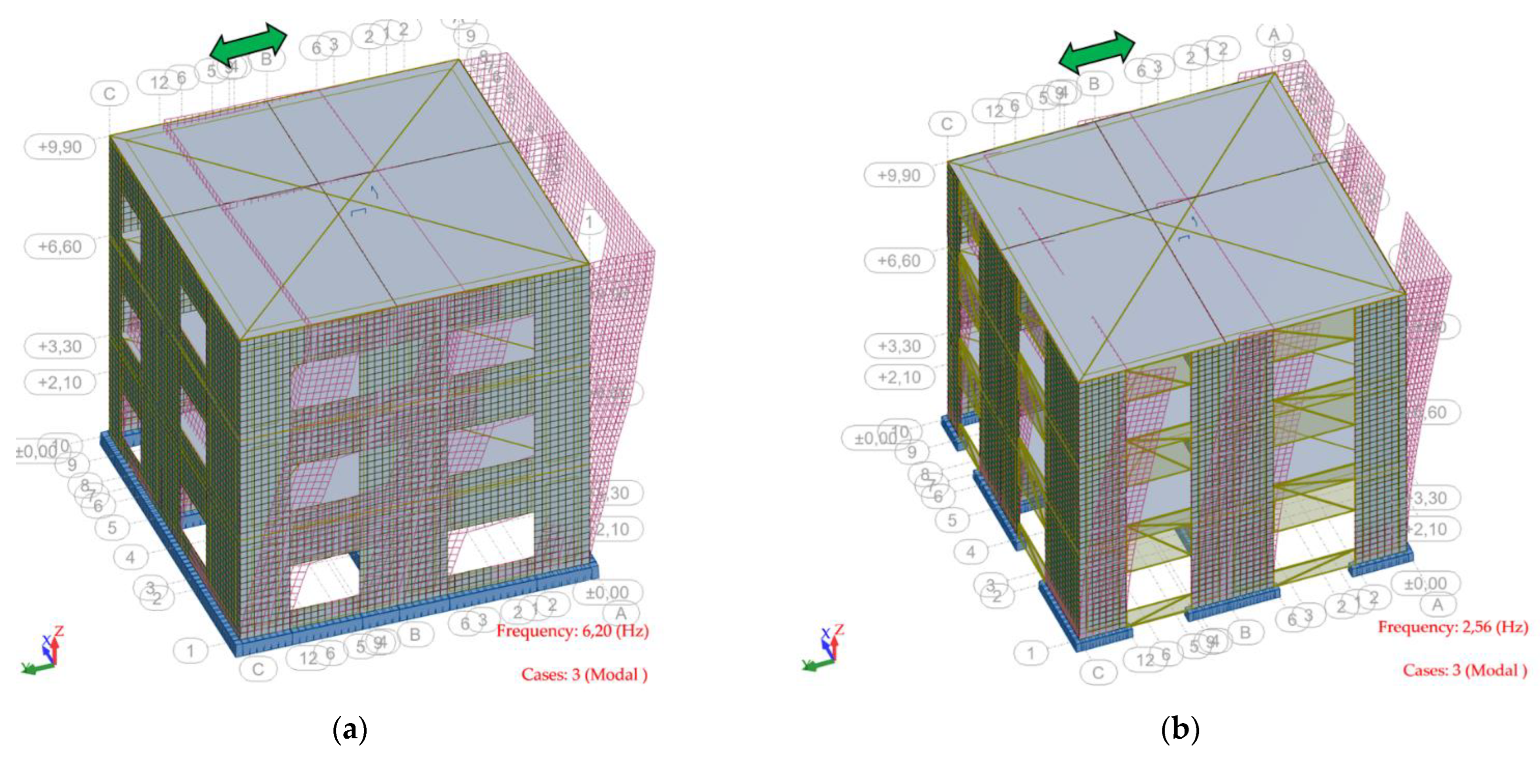
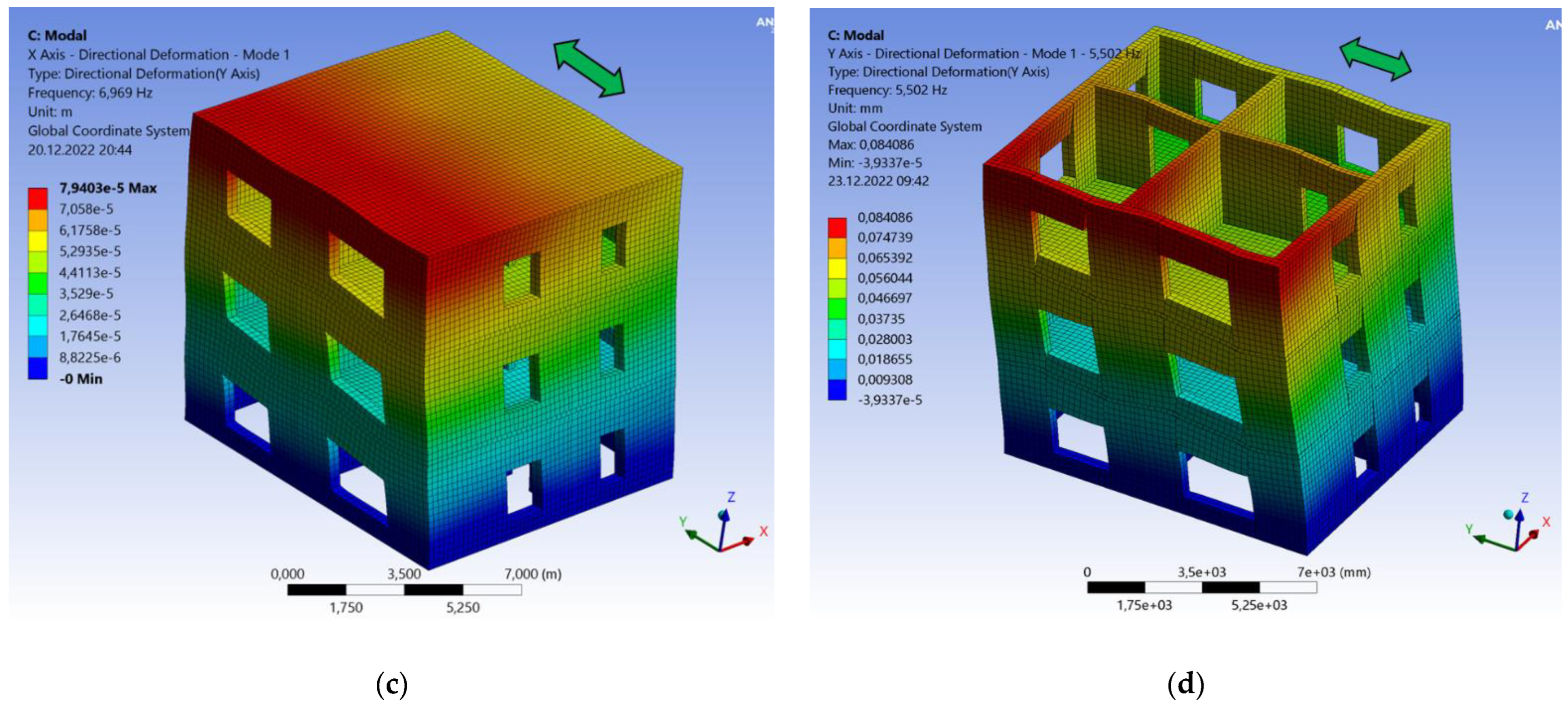
4.1. Modal Analysis Results
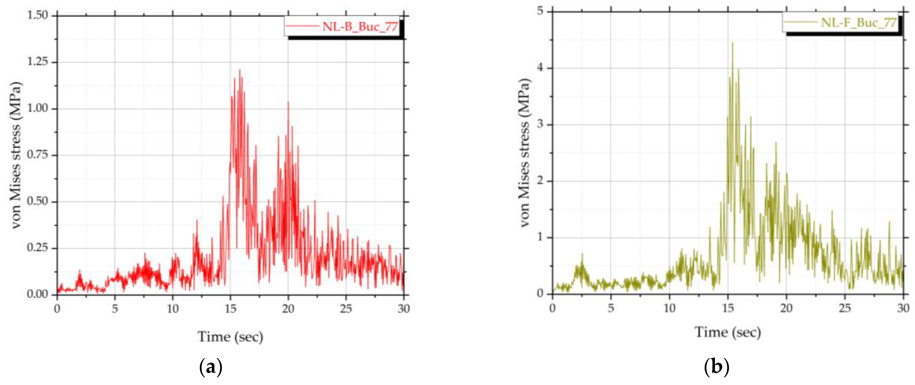
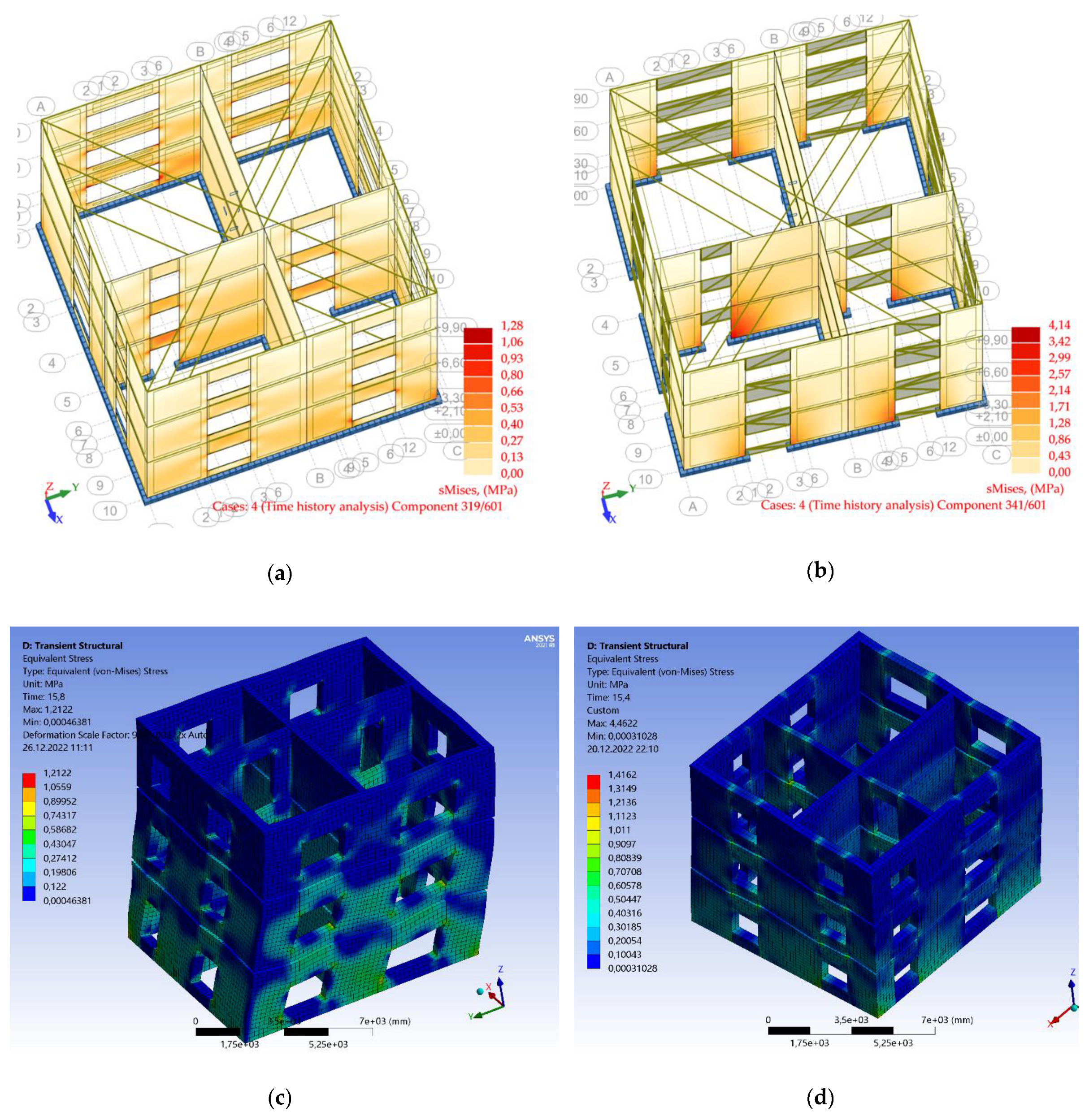
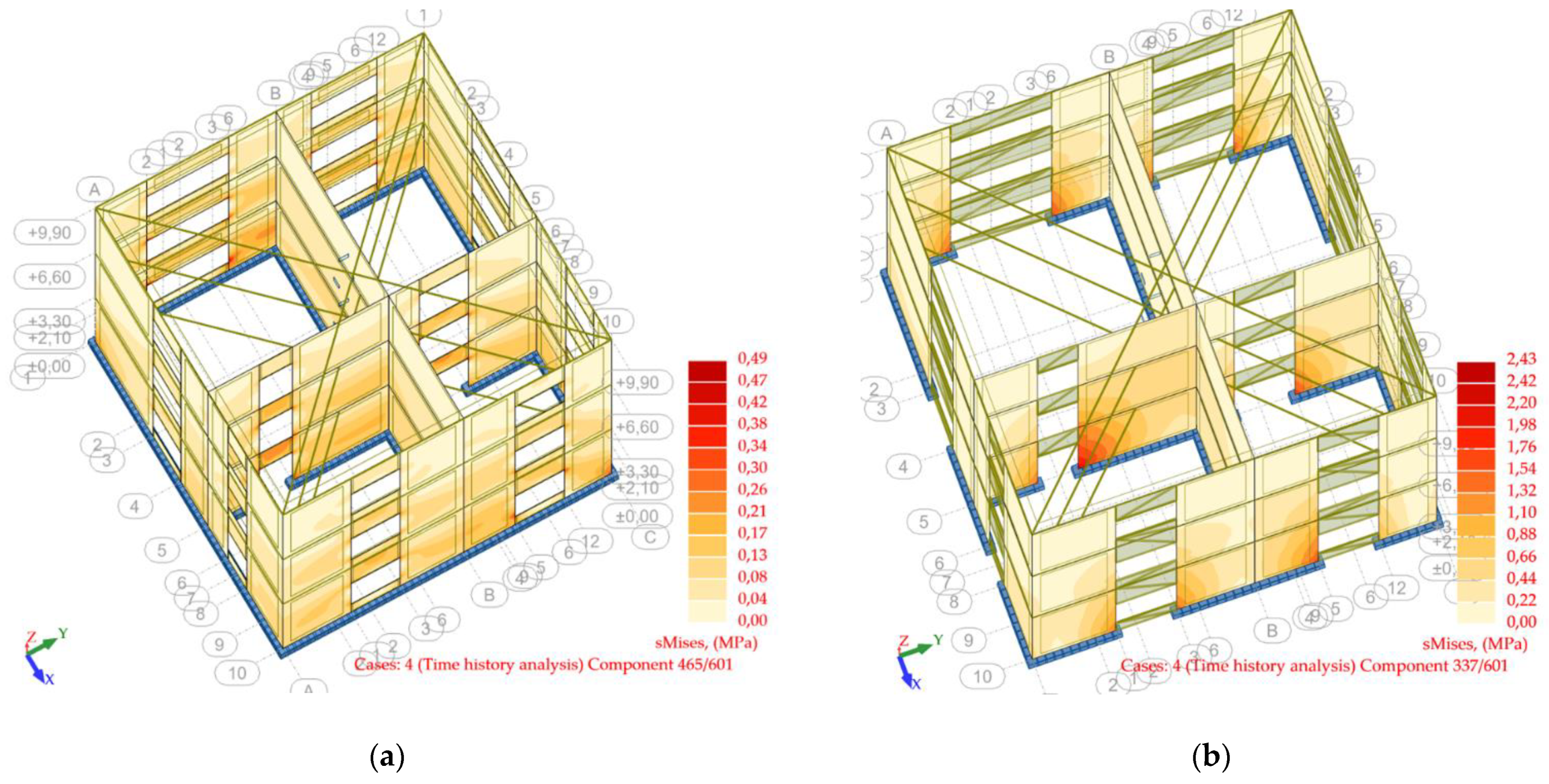
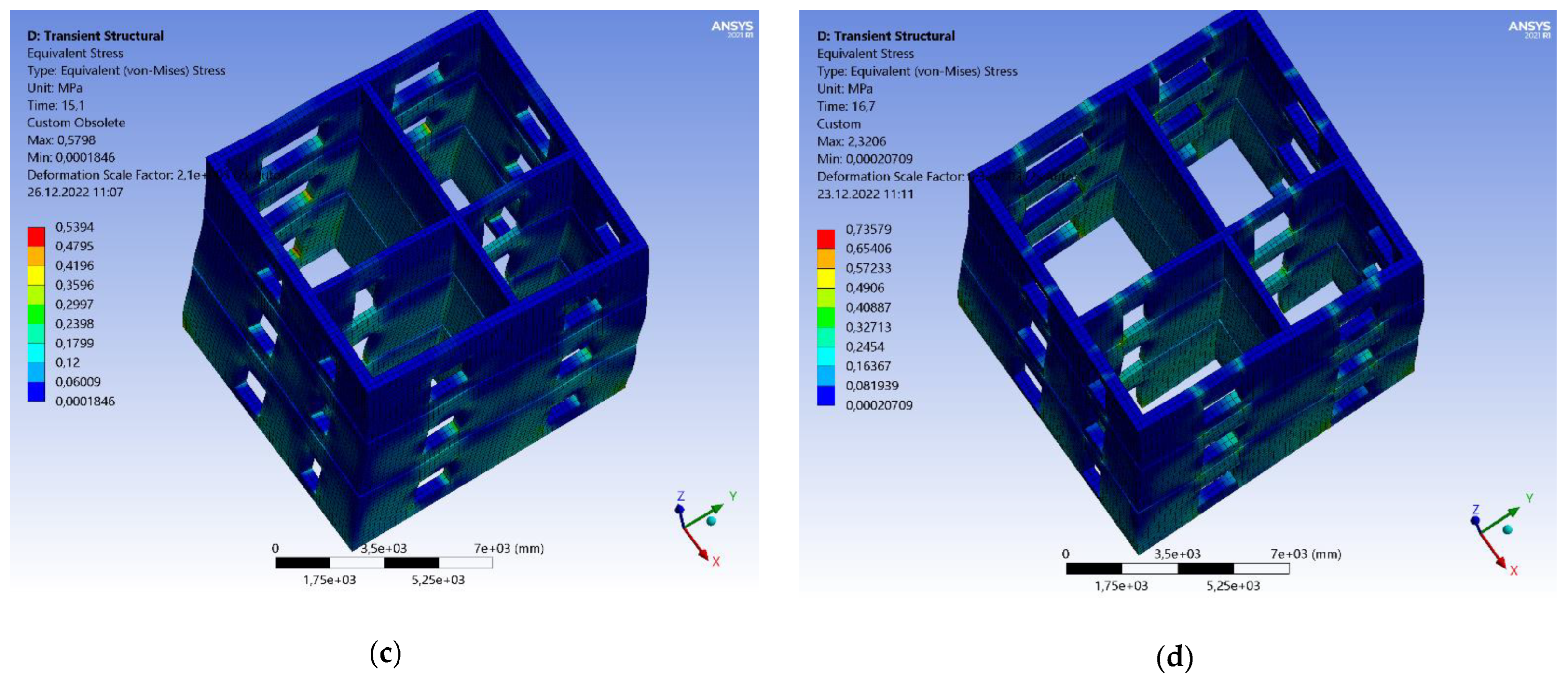
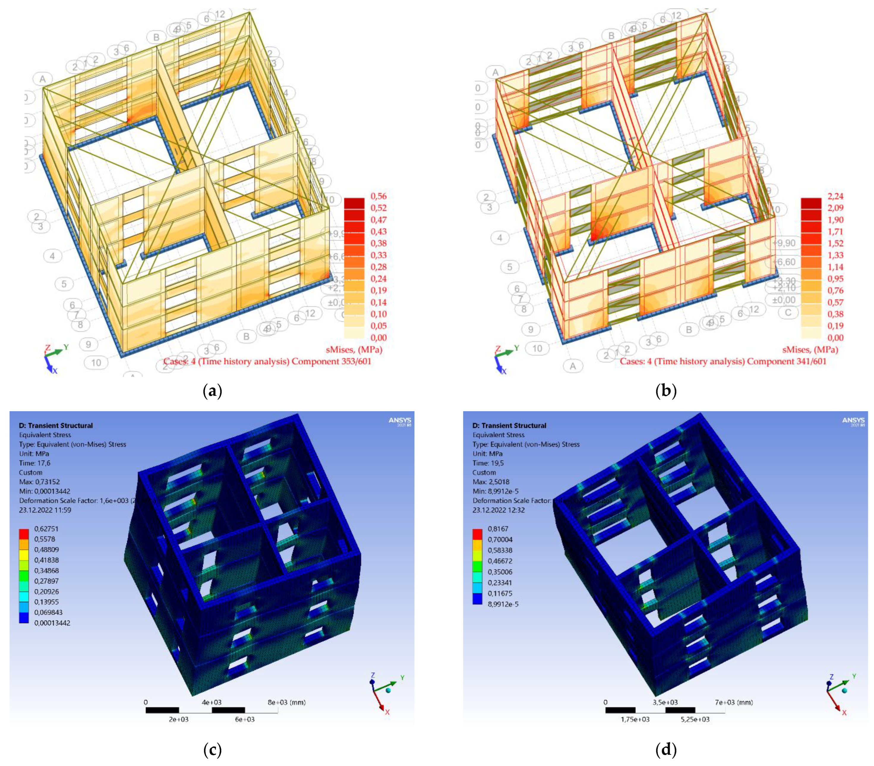
4.2. Time History Analysis Results in Terms of Stresses
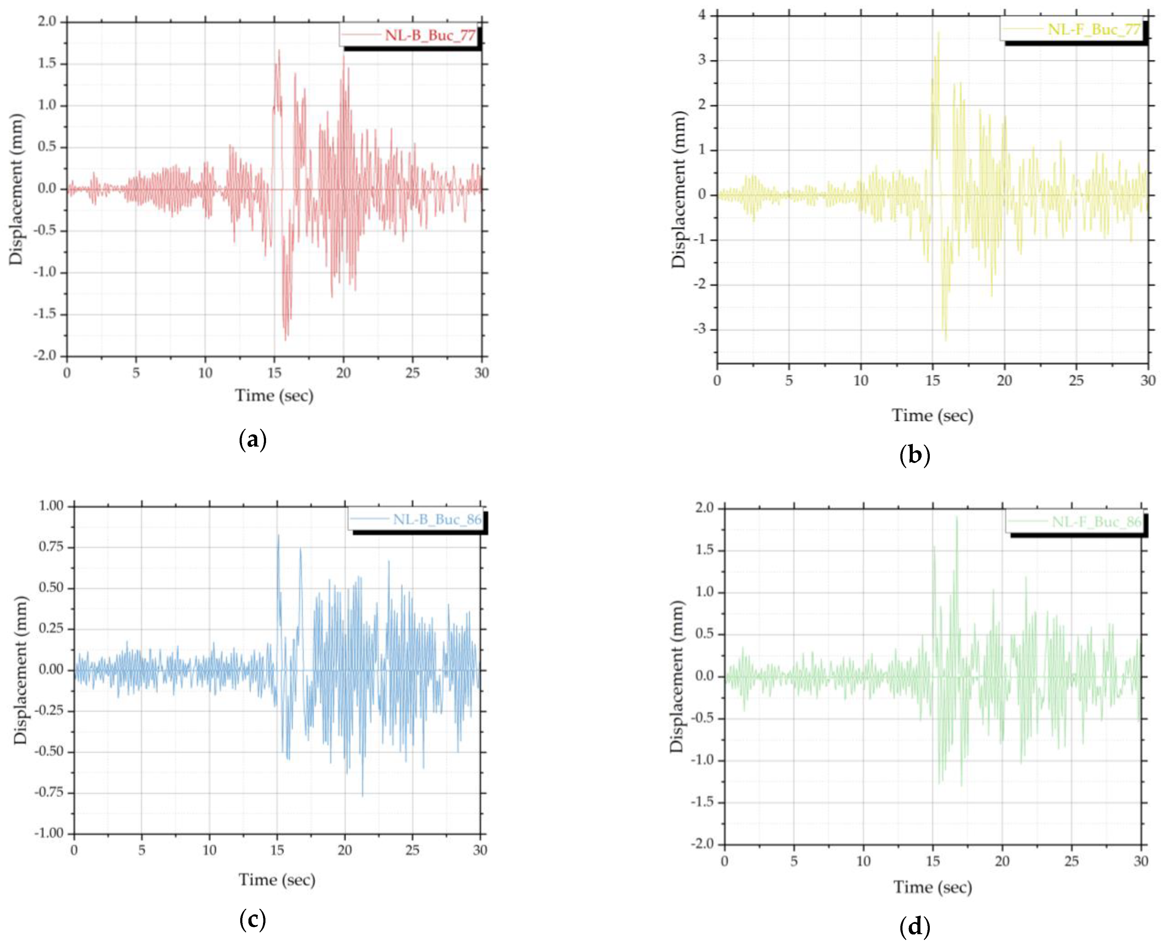
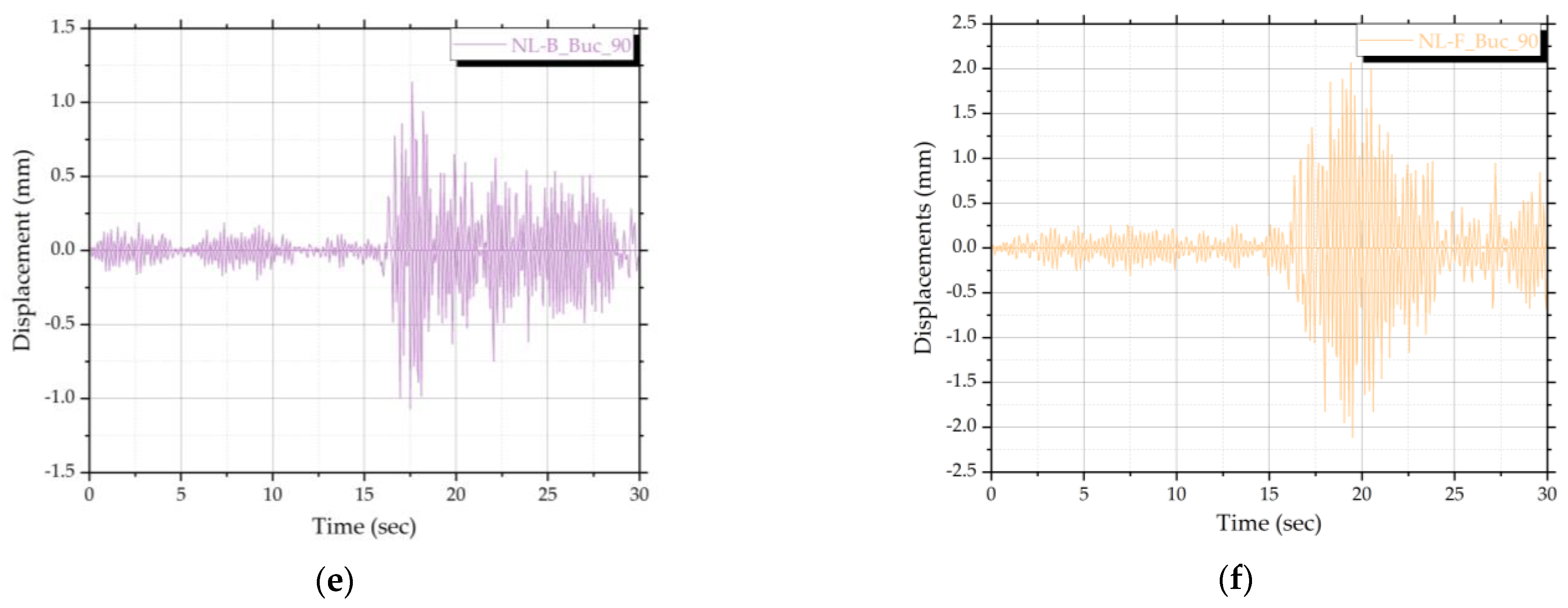
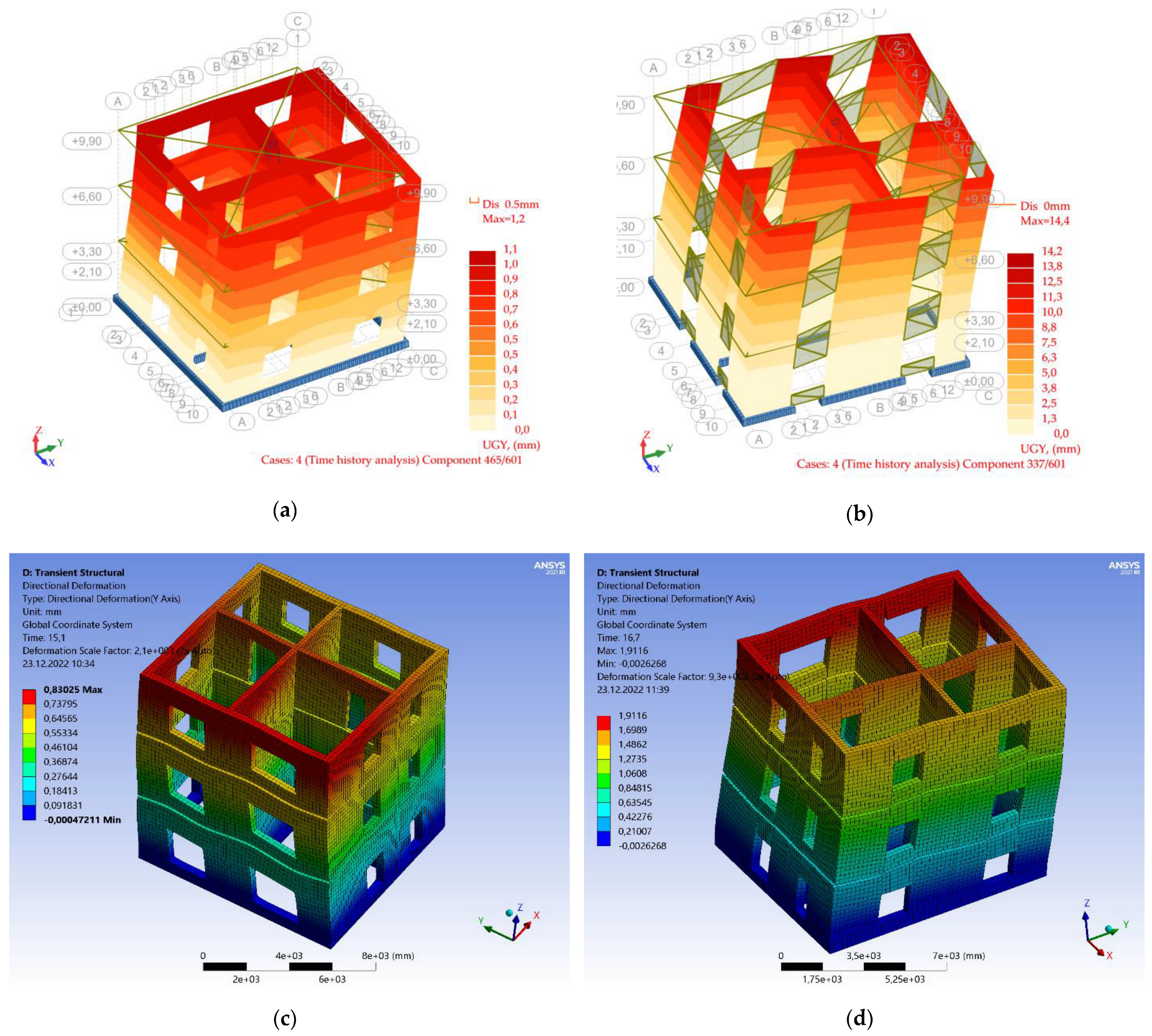
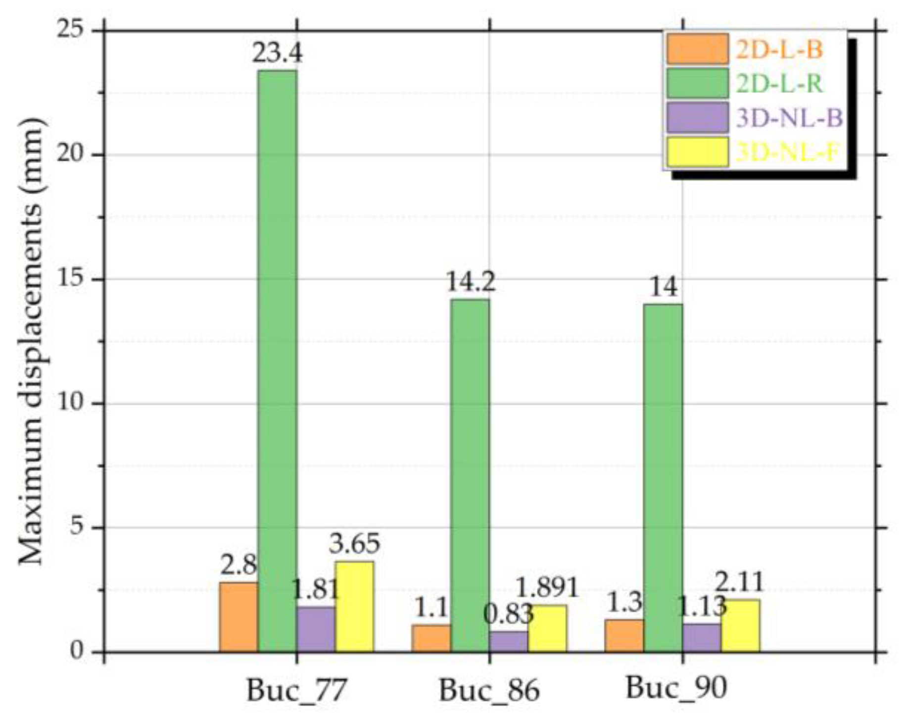
4.3. Time History Analysis Results in Terms of Displacements
5. Conclusions
Author Contributions
Funding
Institutional Review Board Statement
Informed Consent Statement
Data Availability Statement
Conflicts of Interest
References
- Jenkins, R.; Barton, J. Environmental Regulation in the New Global Economy: The Impact of Industry and Competitiveness; Edward Elgar Publishing: Cheltenham, UK, 2002. [Google Scholar]
- KMB Energy Engineering Company Unveils 6 Fundamental Principles of Sustainable Building Design. Available online: https://www.kmbdg.com/news/energy-engineering-company-sustainable-building-design/ (accessed on 26 December 2022).
- Almeida, C.P.; Ramos, A.F.; Silva, J.M. Sustainability Assessment of Building Rehabilitation Actions in Old Urban Centres. Sustain. Cities Soc. 2018, 36, 378–385. [Google Scholar] [CrossRef]
- Almssad, A.; Almusaed, A.; Homod, R.Z. Masonry in the Context of Sustainable Buildings: A Review of the Brick Role in Architecture. Sustainability 2022, 14, 4734. [Google Scholar] [CrossRef]
- Ministerul Dezvoltării, Lucrărilor Publice și Administrației. Masonry Structures Design Code—CR 6—2013. 2013. Available online: https://www.mdlpa.ro/userfiles/reglementari/Domeniul_V/V_9_3_CR_6_2013.pdf (accessed on 30 January 2023).
- Cattari, S.; Beyer, K. Influence of Spandrel Modelling on the Seismic Assessment of Existing Masonry Buildings. In Proceedings of the Tenth Pacific Conference on Earthquake Engineering Building an Earthquake-Resilient Pacific, Sydney, Australia, 6–8 November 2015. [Google Scholar]
- FEMA 356; Pre-Standard and Commentary for the Seismic Rehabilitation of Buildings. American Society of Civil Engineers: Reston, VA, USA, 2000.
- Cattari, S.; Lagomarsino, S. A Strength Criterion for the Flexural Behaviour of Spandrel in Un-Reinforced Masonry Walls. In Proceedings of the 14th World Conference on Earthquake Engineering, Beijing, China, 12–17 October 2008. [Google Scholar]
- Beyer, K.; Mangalathu, S. Review of Strength Models for Masonry Spandrels. Bull. Earthq. Eng. 2012, 11, 521–542. [Google Scholar] [CrossRef]
- Beyer, K.; Dazio, A. Quasi-Static Cyclic Tests on Masonry Spandrels. Earthq. Spectra 2012, 28, 907–929. [Google Scholar] [CrossRef]
- Beyer, K. Peak and Residual Strengths of Brick Masonry Spandrels. Eng. Struct. 2012, 41, 533–547. [Google Scholar] [CrossRef]
- Dazio, A.; Beyer, K. Seismic Behaviour of Different Types of Masonry Spandrels. In Proceedings of the 4th European Conference on Earthquake Engineering, Ohrid, Macedonia, 30 August–3 September 2010. [Google Scholar]
- Ahmad, N.; Ali, M. Displacement-Based Seismic Assessment of Masonry Buildings for Global and Local Failure Mechanisms. Cogent Eng. 2017, 4, 1414576. [Google Scholar] [CrossRef]
- Guerrini, G.; Graziotti, F.; Penna, A.; Magenes, G. Improved Evaluation of Inelastic Displacement Demands for Short- Period Masonry Structures. Earthq. Eng. Struct. Dyn. 2017, 46, 1411–1430. [Google Scholar] [CrossRef]
- Esposito, R.; Messali, F.; Ravenshorst, G.; Schipper, R.; Rots, J. Seismic Assessment of a Lab-Tested Two-Storey Unreinforced Masonry Dutch Terraced House. Bull. Earthq. Eng. 2019, 17, 4601–4623. [Google Scholar] [CrossRef]
- Kim, G.-W.; Song, J.-K.; Jung, S.-J.; Song, Y.-H.; Yoon, T.-H. Lateral Load Distribution Factor for Modal Pushover Analysis. In Proceedings of the Council on Tall Buildings and Urban Habitat, Seoul, Republic of Korea, 10–13 October 2004. [Google Scholar]
- Rostami, A.; Poursha, M. A Lateral Load Distribution for the Static Analysis of Base-Isolated Building Frames under the Effect of Far-Fault and near-Fault Ground Motions. Structures 2021, 34, 2384–2405. [Google Scholar] [CrossRef]
- Quagliarini, E.; Maracchini, G.; Clementi, F. Uses and Limits of the Equivalent Frame Model on Existing Unreinforced Masonry Buildings for Assessing Their Seismic Risk: A Review. J. Build. Eng. 2017, 10, 166–182. [Google Scholar] [CrossRef]
- Dumitraş, M.; Cobîrzan, N.; Dumitraş, D. Considerations Regarding the Analysis of Masonry Walls to Horizontal Loads Using Equivalent Frame Method Building. Bull. Polytech. Inst. Jassy Constr. Archit. Sect. 2013, 59, 41. [Google Scholar]
- Gusella, F.; Orlando, M.; Thiele, K. Evaluation of Rack Connection Mechanical Properties by Means of the Component Method. J. Constr. Steel Res. 2018, 149, 207–224. [Google Scholar] [CrossRef]
- Kasaeian, S.; Usefi, N.; Ronagh, H.; Dareshiry, S. Seismic Performance of CFS Strap-Braced Walls Using Capacity-Based Design Approach. J. Constr. Steel Res. 2020, 174, 106317. [Google Scholar] [CrossRef]
- Soveja, L.; Budescu, M.; Gosav, I. Modelling Methods for Unreinforced Masonry Structures. Bull. Polytech. Inst. Jassy Constr. Archit. Sect. 2013, 59, 19. [Google Scholar]
- Taranu, G. Strengthening of Masonry Arches and Vaults at Historical Monuments/Consolidarea Arcelor si Boltilor din Zidarie la Monumentele Istorice; Loghin, C., Ed.; Politehnium: Iasi, Romania, 2021; ISBN 978-973-621-497-4. [Google Scholar]
- Pleşu, R.; Ţăranu, G.; Covatariu, D.; Grădinariu, I.-D. Strengthening and Rehabilitation Conventional Methods for Masonry Structures. Bul. Inst. Politeh. Sect. Constr. Arhit. 2011, 57, 165. [Google Scholar]
- Venghiac, V.M.; Olariu, C.P.; Budescu, M. Structural Rehabilitation Analyses for a Romanian Cultural Heritage Building Located in Seismic Area. Adv. Eng. Forum 2017, 21, 196–203. [Google Scholar] [CrossRef]
- Pleşu, R.; Taranu, G.; Budescu, M. FEM Analyses of a 1:2 Scale Historical Unreinforced Masonry Building. In Proceedings of the Computational Civil Engineering—CCE2013, International Symposium, Iasi, Romania, 24 May 2013. [Google Scholar]
- Ple, R. Contributii Privind Metodele de Reabilitare a Structurilor din Zidarie/ Contributions Regarding the Rehabilitation Methods of Masonry Structures. Ph.D. Thesis, The “Gheorghe Asachi” Technical University of Iasi, Iasi, Romania, 2013. [Google Scholar]
- Taranu, G.; Toma, I.-O.; Taranu, N. Shake Table Test of a 1:2 Scale Historical Unreinforced Masonry Building. In Proceedings of the 1st Croatian Conference on Earthquake ENgineering, 1 CroCEE, Zagreb, Croatia, 22–24 March 2021. [Google Scholar]
- Ministerul Dezvoltării, Lucrărilor Publice și Administrației. Code for Earthquake Design P100-3/2019 Provisions for the Seismic Assessment of Existing Buildings 2019. Available online: https://www.mdlpa.ro/userfiles/reglementari/Domeniul_I/P100partea%20a%20iiia.pdf (accessed on 14 January 2023).
- Ansys|Engineering Simulation Software. Available online: https://www.ansys.com/ (accessed on 19 October 2021).
- Robot Structural Analysis Professional. Available online: https://www.autodesk.com/products/robot-structural-analysis/overview (accessed on 13 January 2022).
- Ansys Contact Types and Explanations. Available online: https://www.mechead.com/contact-types-and-behaviours-in-ansys/ (accessed on 14 January 2023).
- Casapulla, C.; Portioli, F.; Maione, A.; Landolfo, R. A Macro-Block Model for in-Plane Loaded Masonry Walls with Non-Associative Coulomb Friction. Meccanica 2013, 48, 2107–2126. [Google Scholar] [CrossRef]
- Sassu, M.; Andreini, M.; Casapulla, C.; de Falco, A. Archaeological Consolidation of UNESCO Masonry Structures in Oman: The Sumhuram Citadel of Khor Rori and the Al Balid Fortress. Int. J. Arch. Herit. 2012, 7, 339–374. [Google Scholar] [CrossRef]
- Casapulla, C.; Argiento, L.U.; Maione, A.; Speranza, E. Upgraded Formulations for the Onset of Local Mechanisms in Multi-Storey Masonry Buildings Using Limit Analysis. Structures 2021, 31, 380–394. [Google Scholar] [CrossRef]
- Casapulla, C.; Portioli, F. Experimental and Analytical Investigation on the Frictional Contact Behavior of 3D Masonry Block Assemblages. Constr. Build. Mater. 2015, 78, 126–143. [Google Scholar] [CrossRef]
- Hafner, I.; Lazarević, D.; Kišiček, T.; Stepinac, M. Post-Earthquake Assessment of a Historical Masonry Building after the Zagreb Earthquake–Case Study. Buildings 2022, 12, 323. [Google Scholar] [CrossRef]
- Croce, P.; Landi, F.; Puccini, B.; Martino, M.; Maneo, A. Parametric HBIM Procedure for the Structural Evaluation of Heritage Masonry Buildings. Buildings 2022, 12, 194. [Google Scholar] [CrossRef]
- Manzini, C.F.; Ottonelli, D.; Degli Abbati, S.; Marano, C.; Cordasco, E.A. Modelling the Seismic Response of a 2-Storey URM Benchmark Case Study: Comparison among Different Equivalent Frame Models. Bull. Earthq. Eng. 2022, 20, 2045–2084. [Google Scholar] [CrossRef]
- Croce, P.; Landi, F.; Formichi, P.; Beconcini, M.L.; Puccini, B.; Zotti, V. Non-Linear Methods for the Assessment of Seismic Vulnerability of Masonry Historical Buildings. In Protection of Historical Constructions; Lecture Notes in Civil Engineering; Springer: Cham, Switzerland, 2022; Volume 209. [Google Scholar]
- Asad, M.; Zahra, T.; Thamboo, J.; Song, M. Finite Element Modelling of Reinforced Masonry Walls under Axial Compression. Eng. Struct. 2022, 252, 113594. [Google Scholar] [CrossRef]
- Cannizzaro, F.; Castellazzi, G.; Grillanda, N.; Pantò, B.; Petracca, M. Modelling the Nonlinear Static Response of a 2-Storey URM Benchmark Case Study: Comparison among Different Modelling Strategies Using Two- and Three-Dimensional Elements. Bull. Earthq. Eng. 2022, 20, 2085–2114. [Google Scholar] [CrossRef]
- Beconcini, M.L.; Formichi, P.; Giresini, L.; Landi, F.; Puccini, B.; Croce, P. Modeling Approaches for the Assessment of Seismic Vulnerability of Masonry Structures: The E-PUSH Program. Buildings 2022, 12, 346. [Google Scholar] [CrossRef]
- Cattari, S.; Calderoni, B.; Caliò, I.; Camata, G.; de Miranda, S.; Magenes, G.; Milani, G.; Saetta, A. Nonlinear Modeling of the Seismic Response of Masonry Structures: Critical Review and Open Issues towards Engineering Practice. Bull. Earthq. Eng. 2022, 20, 1939–1997. [Google Scholar] [CrossRef]
- D’Altri, A.M.; Cannizzaro, F.; Petracca, M.; Talledo, D.A. Nonlinear Modelling of the Seismic Response of Masonry Structures: Calibration Strategies. Bull. Earthq. Eng. 2022, 20, 1999–2043. [Google Scholar] [CrossRef]
- EN 1991-1-1; European Committee for Standardization Eurocode 1: Actions on Structures—Part 1-1: General Actions—Densities, Self-Weight, Imposed Loads for Buildings. European Committee for Standardization: Brussels, Belgium, 2002.
- INFP Bridging the Gap between Seismology and Earthquake Engineering: From the Seismicity of Romania towards a Refined Implementation of Seismic Action EN 1998-1 (2004) in Earthquake Resistant Design of Buildings (BIGSEES Project). Available online: http://bigsees.infp.ro/ (accessed on 26 December 2022).
- FEMA 450; Building Seismic Safety Council of the National Institute of Building Sciences NEHRP. Recommended Provisions for Seismic Regulations for New Buildings and Other Structures, Part 1-15. Building Seismic Safety Council of the National Institute of Building Sciences NEHRP: Washington, DC, USA, 2003.
- Chopra, A.K. Dynamics of Structures, 3rd ed.; Pearson Education: Noida, India, 2006. [Google Scholar]
- Ministerul Dezvoltării, Lucrărilor Publice și Administrației. Romania P100-1/2013: Seismic Design Code—Part I: Design Rules for Buildings (in Romanian). 2013. Available online: https://www.mdlpa.ro/userfiles/reglementari/Domeniul_I/I_22_P100_1_2013.pdf (accessed on 26 January 2023). (In Romanian).
- Hartmann, F.; Katz, C. Structural Analysis with Finite Elements; Springer: Berlin, Germany, 2007. [Google Scholar]


| No. | Earthquake–Magnitude | LatN | LongE | h(km) | Date | Mw |
|---|---|---|---|---|---|---|
| 1 | Vrancea M= 7.2 | 45.34 | 26.30 | 109 | 1977.03.04 | 7.5 |
| 2 | Vrancea M = 7.0 | 45.53 | 26.47 | 133 | 1986.08.30 | 7.3 |
| 3 | Vrancea M = 6.7 | 45.82 | 26.90 | 91 | 1990.05.30 | 7.0 |
| 4 | Vrancea M = 6.1 | 45.83 | 26.89 | 79 | 1990.05.31 | 6.4 |
| 5 | Vrancea M = 6.0 | 45.79 | 26.71 | 100 | 2004.10.27 | 6.0 |
| Recorded Seismic Action | 2D Shell Linear | 3D Solids Non-Linear | ||
|---|---|---|---|---|
| Bonded | Rigid Links | Bonded | Frictionless | |
| Bucharest 1977 | 2D-L-B_Buc_77 | 2D-L-R_Buc_77 | 3D-NL-B_Buc_77 | 3D-NL-F_Buc_77 |
| Bucharest 1986 | 2D-L-B_Buc_86 | 2D-L-R_Buc_86 | 3D-NL-B_Buc_86 | 3D-NL-F_Buc_86 |
| Bucharest 1990 | 2D-L-B_Buc_90 | 2D-L-R_Buc_90 | 3D-NL-B_Buc_90 | 3D-NL-F_Buc_90 |
| Concrete Class C16/20 | Density (kg/m3) | 2000 | |
| Young’s Modulus (MPa) | 29,000 | ||
| Masonry homogeneous material | Density (kg/m3) | ||
| Isotropic elasticity | Derive from Young’s modulus and Poisson’s ratio | ||
| Young’s modulus (MPa) | 2310 | ||
| Poisson’s ratio (MPa) | 0.15 | ||
| Bulk modulus (MPa) | 1100 | ||
| Shear modulus (MPa) | 1004 | ||
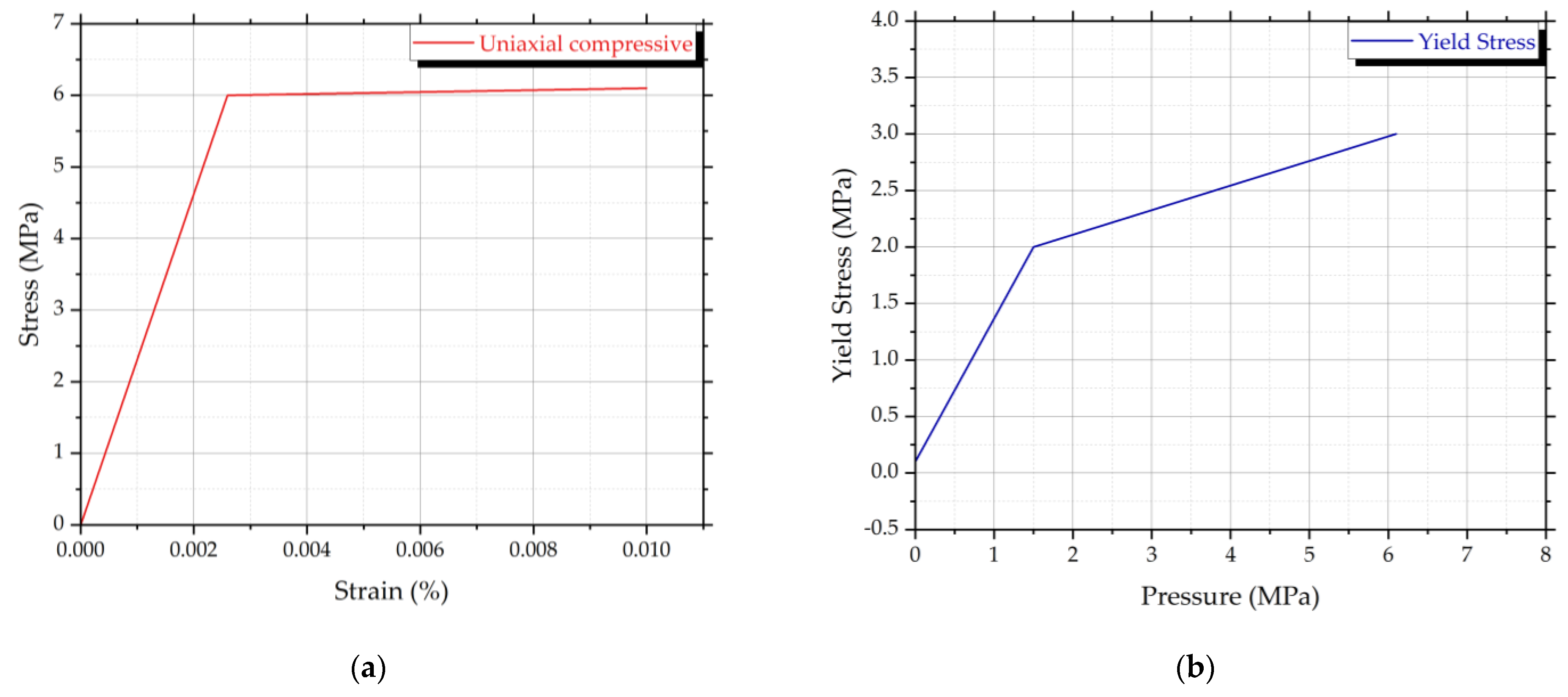
| Uniaxial test data | Compressive stress–strain curve | Figure 9a | |
| Drucker–Prager strength piecewise | Yield stress–pressure curve | Figure 9b | |
| Tensile pressure failure | Maximum tensile pressure (MPa) | −0.1 | |
| Crack softening failure | Flow rule | No Bulking | |
| Fracture energy Gf (J/m2) | 10 | ||
| Load Type | Load Name | Characteristic Load Value |
|---|---|---|
| Permanent | Self-weight:
| 18 kN/m3 25 kN/m3 0.40 kN/m2 |
| Levelling layer + Finishing | 1.40 kN/m2 | |
| Partition walls | 1.25 kN/m2 | |
| Variable | Live load: people, furniture | 1.50 kN/m2 |
| Earthquake Year | Peak Acceleration [m/s2] | Total Duration [sec] | No. of Points | Spaced Interval | Damping [%] |
|---|---|---|---|---|---|
| 1977 | 1.94927 | 40.14 | 2008 | 0.02 | 5 |
| 1986 | 0.66900 | 47.98 | 9596 | 0.005 | 5 |
| 1990 | 9.58 × 10⁻³ | 52.9 | 9870 | 0.005 | 5 |
| Numerical Model | Mode | Period [s] | Frequency [Hz] | Modal Participating Mass Ratio on X Direction | Modal Participating Mass Ratio on Y Direction |
|---|---|---|---|---|---|
| 2D-L-B | 1 | 0.16 | 6.20 | 0.001 | 0.7698 |
| 2D-L-R | 1 | 0.39 | 2.56 | 0.002 | 0.6514 |
| 3D-NL-B | 1 | 0.14 | 6.969 | 0.00073 | 0.746 |
| 3D-NL-F | 1 | 0.18 | 5.502 | 0.0014 | 0.722 |
| Pier | Load Combo | Nd kN | VEd kN | Md kNm | Vf1 kN | Vf2min kN | VRd kN | R3i |
|---|---|---|---|---|---|---|---|---|
| T1 | GSY | −238.7 | 34.359 | 37.585 | 107.16 | 52.842 | 52.842 | 1.5379 |
| T2 | GSY | −452.4 | 93.901 | 138.04 | 265.2 | 96.811 | 96.811 | 1.031 |
| T3 | GSY | −245.6 | 49.703 | 50.712 | 109.63 | 53.534 | 53.534 | 1.0771 |
| T4 | GSY | −153.2 | 17.391 | 20.931 | 69.314 | 34.631 | 34.631 | 1.9913 |
| T5 | GSY | −495.3 | 89.91 | 161.86 | 457.98 | 137.61 | 137.61 | 1.5305 |
| T6 | GSY | −202.1 | 34.27 | 37.309 | 116.44 | 46.587 | 46.587 | 1.3594 |
| T7 | GSY | −223 | 25.557 | 21.418 | 135.22 | 60.908 | 60.908 | 2.3833 |
| T8 | GSY | −466 | 75.102 | 125.63 | 411.98 | 155.35 | 155.35 | 2.0686 |
| T9 | GSY | −168.7 | 25.315 | 41.653 | 80.205 | 45.253 | 45.253 | 1.7876 |
| L1 | GSX | −469.8 | 59.736 | 74.211 | 454.55 | 162.64 | 162.64 | 2.7226 |
| L2 | GSX | −329.7 | 46.359 | 50.011 | 208.57 | 83.695 | 83.695 | 1.8054 |
| L3 | GSX | −166 | 27.966 | 36.663 | 79.114 | 44.942 | 44.942 | 1.607 |
| L4 | GSX | −174.2 | 14.891 | 17.522 | 76.726 | 36.715 | 36.715 | 2.4656 |
| L5 | GSX | −556.4 | 96.921 | 167.61 | 582.77 | 155.11 | 155.11 | 1.6004 |
| L6 | GSX | −147.2 | 23.479 | 20.519 | 67.093 | 34.009 | 34.009 | 1.4485 |
| L7 | GSX | −346.1 | 32.393 | 30.262 | 246.15 | 100.83 | 100.83 | 3.1127 |
| L8 | GSX | −426.1 | 56.702 | 82.537 | 318.6 | 124.67 | 124.67 | 2.1988 |
| L9 | GSX | −117.8 | 10.223 | 17.933 | 40.442 | 32.131 | 32.131 | 3.1429 |
| R3T = 1.53427 | R3 =1.53427 | Risk class RsIV | ||||||
| R3L = 2.101445 | ||||||||
| Pier | Load Combo | Nd kN | VEd kN | Md kNm | Vf1 kN | Vf2min kN | VRd kN | R3i |
|---|---|---|---|---|---|---|---|---|
| T1 | GSY | −239.3 | 35.572 | 38.29 | 107.38 | 52.903 | 52.903 | 1.4872 |
| T2 | GSY | −451.2 | 95.285 | 141.27 | 264.69 | 96.691 | 96.691 | 1.0147 |
| T3 | GSY | −243.8 | 50.832 | 51.386 | 108.98 | 53.353 | 53.353 | 1.0496 |
| T4 | GSY | −152.8 | 16.283 | 20.013 | 69.159 | 34.588 | 34.588 | 2.1241 |
| T5 | GSY | −495.4 | 85.6 | 157.09 | 458.01 | 137.62 | 137.62 | 1.6067 |
| T6 | GSY | −204.2 | 32.553 | 35.895 | 117.4 | 46.807 | 46.807 | 1.4378 |
| T7 | GSY | −218 | 21.808 | 19.138 | 132.59 | 60.304 | 60.304 | 2.7651 |
| T8 | GSY | −464.7 | 67.786 | 117.47 | 411.07 | 155.16 | 155.16 | 2.2889 |
| T9 | GSY | −164.9 | 23.128 | 40.334 | 78.653 | 44.81 | 44.81 | 1.9374 |
| L1 | GSX | −467.3 | 55.545 | 71.296 | 452.52 | 162.23 | 162.23 | 2.9208 |
| L2 | GSX | −329.3 | 44.195 | 47.998 | 208.4 | 83.658 | 83.658 | 1.8929 |
| L3 | GSX | −166.7 | 26.761 | 35.973 | 79.404 | 45.025 | 45.025 | 1.6825 |
| L4 | GSX | −173.8 | 14.017 | 16.836 | 76.579 | 36.674 | 36.674 | 2.6162 |
| L5 | GSX | −556 | 93.282 | 163.70 | 582.47 | 155.06 | 155.06 | 1.6622 |
| L6 | GSX | −148.6 | 22.591 | 19.845 | 67.611 | 34.154 | 34.154 | 1.5118 |
| L7 | GSX | −345.3 | 31.125 | 29.199 | 245.69 | 100.73 | 100.73 | 3.2361 |
| L8 | GSX | −425.7 | 55.096 | 81.327 | 318.34 | 124.61 | 124.61 | 2.2618 |
| L9 | GSX | −117.1 | 9.9959 | 17.790 | 40.211 | 32.039 | 32.039 | 3.2052 |
| R3T = 1.59063 | R3 = 1.59063 | Risk class RsIV | ||||||
| R3L = 2.19556 | ||||||||
| Pier | Load Combo | Nd kN | VEd kN | Md kNm | Vf1 kN | Vf2min kN | VRd kN | R3i |
|---|---|---|---|---|---|---|---|---|
| T1 | GSY | −227.8 | 64.85 | 68.83 | 103.1 | 51.73 | 51.730 | 0.797 |
| T2 | GSY | −442.8 | 157.1 | 234.8 | 261.1 | 95.850 | 95.850 | 0.609 |
| T3 | GSY | −237.3 | 80.11 | 81.41 | 106.6 | 52.70 | 52.703 | 0.657 |
| T4 | GSY | −150.07 | 31.14 | 35.01 | 68.14 | 34.304 | 34.304 | 1.101 |
| T5 | GSY | −488.4 | 145 | 273.8 | 453.5 | 136.713 | 136.71 | 0.942 |
| T6 | GSY | −192.31 | 52.30 | 61.93 | 111.8 | 45.5482 | 45.548 | 0.870 |
| T7 | GSY | −188.20 | 44.64 | 49.54 | 116.6 | 56.5789 | 56.578 | 1.267 |
| T8 | GSY | −456.71 | 117.5 | 201.5 | 405.3 | 153.937 | 153.93 | 1.309 |
| T9 | GSY | −128.80 | 36.54 | 57.20 | 63.19 | 40.2977 | 40.297 | 1.102 |
| L1 | GSX | −435.52 | 99.49 | 147.8 | 427.0 | 157.184 | 157.18 | 1.579 |
| L2 | GSX | −323.76 | 68.95 | 79.58 | 205.5 | 83.0144 | 83.014 | 1.203 |
| L3 | GSX | −143.07 | 39.73 | 48.70 | 69.41 | 42.1377 | 42.137 | 1.060 |
| L4 | GSX | −169.05 | 24.08 | 28.51 | 74.94 | 36.2124 | 36.212 | 1.503 |
| L5 | GSX | −537.33 | 145.3 | 282.7 | 568.6 | 152.614 | 152.61 | 1.050 |
| L6 | GSX | −145.53 | 34.10 | 31.54 | 66.46 | 33.833 | 33.833 | 0.992 |
| L7 | GSX | −327.63 | 58.86 | 69.23 | 235.3 | 98.377 | 98.377 | 1.671 |
| L8 | GSX | −420.64 | 86.93 | 134.3 | 315.3 | 123.937 | 123.93 | 1.425 |
| L9 | GSX | −103.75 | 15.69 | 23.39 | 36.16 | 30.411 | 30.411 | 1.937 |
| R3T = 0.91535 | R3 = 0.91535 | Risk class RsIV | ||||||
| R3L = 1.32193 | ||||||||
| Pier | Load Combo | Nd kN | VEd kN | Md kNm | Vf1 kN | Vf2min kN | VRd kN | R3i |
|---|---|---|---|---|---|---|---|---|
| T1 | GSY | −71.72 | 36.943 | 58.725 | 36.735 | 11.731 | 11.731 | 0.3175 |
| T2 | GSY | −366.9 | 62.793 | 223.4 | 226.96 | 87.884 | 87.884 | 1.3996 |
| T3 | GSY | −90.54 | 30.765 | 63.959 | 45.733 | 14.811 | 14.811 | 0.4814 |
| T4 | GSY | −97.67 | 20.645 | 33.115 | 47.261 | 28.379 | 28.379 | 1.3746 |
| T5 | GSY | −456.1 | 101.59 | 315.91 | 431.85 | 132.42 | 132.42 | 1.3035 |
| T6 | GSY | −139.3 | 35.815 | 59.212 | 85.229 | 39.47 | 39.47 | 1.1021 |
| T7 | GSY | −192.1 | 25.259 | 43.538 | 118.76 | 57.084 | 57.084 | 2.26 |
| T8 | GSY | −420.8 | 71.91 | 199.61 | 379.24 | 148.35 | 148.35 | 2.063 |
| T9 | GSY | −122 | 17.755 | 45.817 | 60.147 | 39.384 | 39.384 | 2.2182 |
| L1 | GSX | −441.9 | 78.313 | 167.06 | 432.22 | 158.22 | 158.22 | 2.0203 |
| L2 | GSX | −297.6 | 42.773 | 77.403 | 191.92 | 79.922 | 79.922 | 1.8685 |
| L3 | GSX | −159.5 | 24.211 | 41.718 | 76.413 | 44.167 | 44.167 | 1.8242 |
| L4 | GSX | −126.5 | 17.853 | 27.705 | 59.131 | 31.774 | 31.774 | 1.7798 |
| L5 | GSX | −538.5 | 111.44 | 326.13 | 569.52 | 152.77 | 152.77 | 1.3709 |
| L6 | GSX | −104.8 | 18.262 | 26.619 | 50.284 | 29.255 | 29.255 | 1.602 |
| L7 | GSX | −315.3 | 42.122 | 76.665 | 227.98 | 96.707 | 96.707 | 2.2959 |
| L8 | GSX | −386 | 55.798 | 140.07 | 294.44 | 119.18 | 119.18 | 2.136 |
| L9 | GSX | −110.5 | 7.8918 | 17.913 | 38.235 | 31.248 | 31.248 | 3.9595 |
| R3T = 1.38674 | R3 = 1.38674 | Risk class RsIV | ||||||
| R3L = 1.86434 | ||||||||
| Pier | Load Combo | Nd kN | VEd kN | Md kNm | Vf1 kN | Vf2min kN | VRd kN | R3i |
|---|---|---|---|---|---|---|---|---|
| T1 | GSY | −93.45 | 44.607 | 71.304 | 47.1 | 15.287 | 15.287 | 0.3427 |
| T2 | GSY | −358.5 | 73.021 | 271.45 | 222.92 | 54.538 | 54.538 | 0.7469 |
| T3 | GSY | −46.33 | 38.515 | 76.594 | 24.175 | 7.5782 | 7.5782 | 0.1968 |
| T4 | GSY | −103.4 | 22.42 | 36.421 | 49.685 | 29.082 | 29.082 | 1.2971 |
| T5 | GSY | −448.3 | 109.8 | 356.52 | 426.48 | 131.38 | 131.38 | 1.1965 |
| T6 | GSY | −131.8 | 38.257 | 65.985 | 81.192 | 38.53 | 38.53 | 1.0071 |
| T7 | GSY | −168.6 | 22.474 | 47.338 | 105.74 | 53.992 | 53.992 | 2.4024 |
| T8 | GSY | −418.1 | 69.725 | 205.78 | 377.21 | 147.92 | 147.92 | 2.1215 |
| T9 | GSY | −129.1 | 16.011 | 47.72 | 63.308 | 40.332 | 40.332 | 2.5191 |
| L1 | GSX | −439.6 | 64.487 | 141.87 | 430.29 | 157.83 | 157.83 | 2.4475 |
| L2 | GSX | −294.3 | 36.795 | 66.837 | 190.12 | 79.514 | 79.514 | 2.161 |
| L3 | GSX | −157.8 | 20.946 | 37.999 | 75.678 | 43.955 | 43.955 | 2.0985 |
| L4 | GSX | −133.8 | 15.274 | 24.252 | 61.98 | 32.575 | 32.575 | 2.1328 |
| L5 | GSX | −543.4 | 97.423 | 286.85 | 573.19 | 153.41 | 153.41 | 1.5747 |
| L6 | GSX | −110 | 15.62 | 23.184 | 52.449 | 29.877 | 29.877 | 1.9128 |
| L7 | GSX | −314.6 | 35.6 | 65.57 | 227.51 | 96.6 | 96.6 | 2.7135 |
| L8 | GSX | −382.6 | 48.967 | 124.95 | 292.38 | 118.72 | 118.72 | 2.4245 |
| L9 | GSX | −111.6 | 6.8775 | 16.759 | 38.573 | 31.384 | 31.384 | 4.5632 |
| R3T = 1.19273 | R3 = 1.19273 | Risk class RsIV | ||||||
| R3L = 2.17513 | ||||||||
| Pier | Load Combo | Nd kN | VEd kN | Md kNm | Vf1 kN | Vf2min kN | VRd kN | R3i |
|---|---|---|---|---|---|---|---|---|
| T1 | GSY | 120.27 | 75.719 | 124.23 | 59.391 | 19.673 | 19.673 | 0.2598 |
| T2 | GSY | −322 | 123.94 | 465.17 | 204.68 | 52.679 | 52.679 | 0.425 |
| T3 | GSY | 92.971 | 69.868 | 129.72 | 46.873 | 15.208 | 15.208 | 0.2177 |
| T4 | GSY | −44.71 | 36.741 | 59.344 | 22.979 | 7.3131 | 7.3131 | 0.199 |
| T5 | GSY | −408.1 | 177.07 | 595.65 | 397.52 | 66.752 | 66.752 | 0.377 |
| T6 | GSY | −82.31 | 60.748 | 110.79 | 53.017 | 13.464 | 13.464 | 0.2216 |
| T7 | GSY | −108.5 | 31.906 | 84.892 | 70.484 | 17.743 | 17.743 | 0.5561 |
| T8 | GSY | −385.2 | 100.62 | 312.39 | 352.31 | 142.59 | 142.59 | 1.4171 |
| T9 | GSY | −15.58 | 20.313 | 67.073 | 8.3103 | 2.5481 | 2.5481 | 0.1254 |
| L1 | GSX | −424.3 | 123.72 | 275.11 | 417.83 | 155.36 | 155.36 | 1.2557 |
| L2 | GSX | −273.2 | 63.076 | 118.32 | 178.67 | 76.912 | 76.912 | 1.2194 |
| L3 | GSX | −120.5 | 34.279 | 57.096 | 59.506 | 39.19 | 39.19 | 1.1432 |
| L4 | GSX | −105.8 | 27.576 | 42.888 | 50.701 | 29.375 | 29.375 | 1.0652 |
| L5 | GSX | −505.1 | 166.37 | 523.93 | 543.81 | 146.85 | 146.85 | 0.8827 |
| L6 | GSX | −83.88 | 28.266 | 41.727 | 41.246 | 25.642 | 25.642 | 0.9072 |
| L7 | GSX | −295.6 | 71.656 | 138.11 | 215.92 | 93.963 | 93.963 | 1.3113 |
| L8 | GSX | −362.2 | 86.458 | 224.59 | 279.59 | 115.82 | 115.82 | 1.3396 |
| L9 | GSX | −98.56 | 13.039 | 23.952 | 34.55 | 29.751 | 29.751 | 2.2817 |
| R3T = 0.48495 | R3 = 0.48495 | Risk class RsII | ||||||
| R3L =1.16019 | ||||||||
| Pier | Load Combo | VEd kN | Vf1 kN | Vf2min kN | VRd kN | R3i | |
|---|---|---|---|---|---|---|---|
| T1 | GSY | 59.97 | 26.69 | 46.7 | 26.69 | 0.445 | |
| T2 | GSY | 134.97 | 57.5 | 74.1 | 57.5 | 0.426 | |
| T3 | GSY | 59.97 | 26.69 | 46.7 | 26.69 | 0.445 | |
| T4 | GSY | 53.43 | 17.42 | 30.3 | 17.42 | 0.326 | |
| T5 | GSY | 325 | 99.98 | 81.9 | 81.9 | 0.252 | |
| T6 | GSY | 95.61 | 28.78 | 39.1 | 28.78 | 0.301 | |
| T7 | GSY | 166.05 | 36.2 | 46.9 | 36.2 | 0.218 | |
| T8 | GSY | 364.28 | 94.36 | 81.6 | 81.6 | 0.224 | |
| T9 | GSY | 93.18 | 23.67 | 39.9 | 23.67 | 0.254 | |
| L1 | GSX | 418.93 | 108.23 | 86.3 | 86.3 | 0.206 | |
| L2 | GSX | 172.43 | 55.87 | 72.0 | 55.87 | 0.324 | |
| L3 | GSX | 77.61 | 23.67 | 39.9 | 23.67 | 0.305 | |
| L4 | GSX | 41.57 | 17.42 | 30.3 | 17.42 | 0.419 | |
| L5 | GSX | 324.12 | 127.91 | 92.7 | 92.7 | 0.286 | |
| L6 | GSX | 41.51 | 17.56 | 30.6 | 17.56 | 0.423 | |
| L7 | GSX | 144.37 | 53.85 | 57.2 | 53.85 | 0.373 | |
| L8 | GSX | 170.47 | 69.38 | 70.0 | 69.38 | 0.407 | |
| L9 | GSX | 21.67 | 12.22 | 28.7 | 12.22 | 0.564 | |
| R3T = 0.258 | R3 = 0.257 | Risk class RsI | |||||
| R3L =0.257 | |||||||
Disclaimer/Publisher’s Note: The statements, opinions and data contained in all publications are solely those of the individual author(s) and contributor(s) and not of MDPI and/or the editor(s). MDPI and/or the editor(s) disclaim responsibility for any injury to people or property resulting from any ideas, methods, instructions or products referred to in the content. |
© 2023 by the authors. Licensee MDPI, Basel, Switzerland. This article is an open access article distributed under the terms and conditions of the Creative Commons Attribution (CC BY) license (https://creativecommons.org/licenses/by/4.0/).
Share and Cite
Venghiac, V.-M.; Neagu, C.-P.; Taranu, G.; Rotaru, A. Time History Analyses of a Masonry Structure for a Sustainable Technical Assessment According to Romanian Design Codes. Sustainability 2023, 15, 2932. https://doi.org/10.3390/su15042932
Venghiac V-M, Neagu C-P, Taranu G, Rotaru A. Time History Analyses of a Masonry Structure for a Sustainable Technical Assessment According to Romanian Design Codes. Sustainability. 2023; 15(4):2932. https://doi.org/10.3390/su15042932
Chicago/Turabian StyleVenghiac, Vasile-Mircea, Cerasela-Panseluta Neagu, George Taranu, and Ancuta Rotaru. 2023. "Time History Analyses of a Masonry Structure for a Sustainable Technical Assessment According to Romanian Design Codes" Sustainability 15, no. 4: 2932. https://doi.org/10.3390/su15042932
APA StyleVenghiac, V.-M., Neagu, C.-P., Taranu, G., & Rotaru, A. (2023). Time History Analyses of a Masonry Structure for a Sustainable Technical Assessment According to Romanian Design Codes. Sustainability, 15(4), 2932. https://doi.org/10.3390/su15042932