SOS-Based Nonlinear Observer Design for Simultaneous State and Disturbance Estimation Designed for a PMSM Model

Abstract

In this study, a type of nonlinear observer design is studied for a class of nonlinear systems. For the construction of the nonlinear observer, SOS-based optimization tools are utilized, which for some nonlinear dynamical systems have the advantage of transforming the problem into a more tractable one. The general problem of nonlinear observer design is translated into an SOS polynomial optimization which can be turned into an SDP problem. For a study problem, simultaneous state and disturbance estimation is considered, a cascaded nonlinear observer using a certain parameterization is constructed, and computation techniques are discussed. Cascade nonlinear observer structure is a design strategy that decomposes the problem into its components resulting in dimension reduction. In this paper, SOS-based methods using the cascade design technique are represented, and a simultaneous state and disturbance signal online estimation algorithm is constructed. The method with its smaller components is given in detail, the efficacy of the method is demonstrated by means of numerical simulations performed in MATLAB, and the observer is designed using numerical optimization tools YALMIP, MOSEK, and PENLAB.

1. Introduction

In the era of smart grids and sustainability, renewable energy sources have become more popular, requiring certain advanced forecasting methods to estimate and monitor the operation to maximize the efficiency and stability of the overall system [1]. A PMSM (Permanent Magnet Synchronous Motor) is a type of electrical motor that is used in EVs, and some variations of it are used in energy harvesting, such as the ones used in wind and tidal sources [2,3,4]. These types of harvesting mechanisms require estimation algorithms to be used in a general control algorithm and system monitoring purposes [5]. In this paper, SOS (Sum of Squares) programming-based nonlinear observer design is considered. In addition to state estimation, disturbance estimation is also studied. The resulting nonlinear observer design is detailed, with an emphasis on the parameterization and the computational aspect of the terms.

Estimation methods have gained prominence with the advent of control methods and the need to maximize efficiency and guarantee the safety of operations in the face of disturbance signals [6]. There are estimation algorithms that are used in nonlinear system state estimation, some of which can be listed as EKF (Extended Kalman Filter) [7], UKF (Unscented Kalman Filter) [8], PF (Particle Filter) [9], MHE (Moving Horizon Estimator) [10,11], SMO (Sliding Mode Observer) [12], HGO (High Gain Observer) [13], Gain scheduling LTI-based observers [14], TS (Takagi–Sugeno) observers [15], adaptive observers [16], ESO (Extended State Observer) [17], and multiple model observers [18]. EKF tends to be the one that results in a systematic design procedure. Although EKF results in accurate estimation performance for non-problematic nonlinear systems depending on the noise and the initial condition terms that can affect the operation, some numerical problems can arise during the estimation process and the error signals might diverge, which requires some additional control algorithms to be implemented that monitor the health of the estimations and the stability of the error dynamics [19]. UKF and PF are variations of EKF whose main focus is to address the non-gaussian process and measurement noise terms that EKF tolerates to a certain extent [20]. In the presence of nonlinear dynamics, the usual assumptions that enable KF (Kalman Filter) to operate efficiently no longer hold, and the PDF of the noise terms evolves during the operation. PF mainly focuses on this aspect of the problem, and consistent construction of the estimated PDF (Probability Density Function) profile of the noise terms is performed in each sampling step which has a computational price that cannot be tolerated by high dimensional nonlinear dynamical systems [21]. MHE is a different type of estimation algorithm that does not depend on an observer design. Instead, MHE considers the problem of state estimation a type of estimation that can be formulated and solved by employing online solvers to produce an estimate which is computed to minimize some stated objective term. That type of approach, although different from the usual controller or observer design, has the advantage of resulting in a tractable observer design method. With the help of specific nonlinear optimization techniques, nonlinear state estimation can be performed quite efficiently. In systems where there are symmetrical structures or intrinsic information is known a priori, explicit MHE methods can be used, as in the case of explicit MPC (Model Predictive Control), where a controller is designed for each specified region in the state space, and explicit MHE results in a set of observers, each of which is valid in a stated region in the state space—a technique that bridges the area of online computational methods and classical controller design techniques [22,23]. SMO is a nonlinear observer algorithm as its controller counterpart; it employs discontinuous functions and high gains to dominate the terms that prevent the stability of the error dynamics. SMO, due to its structure, has the ability to tolerate the exogenous signals that may deteriorate the estimation accuracy, especially if the exogenous signals enter the system through the dynamics of the measured states [24]. HGO is an observer like in SMO; it utilizes discontinuous terms to eliminate the obstructing terms. HGO requires the dynamical system to have a triangular form that limits the systems to which it can be implemented but results in a straightforward design technique [25]. TS observers are another observer type that provides a systematic approach to constructing the observer. It directly uses the information on the state space region that the system operates and, using Luenberger Observer-like structure, proposes an adaptive observer that is parameterized. The terms are computed using the LMI (Linear Matrix Inequality) optimization methods that are used in constructing LTI controllers and observers. In a way, it attempts to reduce the nonlinear observer problem into a set of linear observer design problems. The method works especially well when the system allows expressing the premise variables that can be considered as the scheduling variables in terms of the measurement signals [26]. There are extensions of TS observer design that suggest expressing the system using the polynomial terms that can be exploited using SOS optimization tools, and for low dimensional problems, it offers a clear approach [27]. Adaptive observers are mainly constructed where there is an uncertain term that prevents conventional observer design techniques from being implemented, and the observer is required to account for this parameter uncertainty. As in the case of adaptive controller design, Barbalat’s Lemma and variations thereof are used to construct the observer that results in stable error dynamics [28].

Observer design mainly depends on the nonlinearity present in the system, which can be an isolated nonlinearity that can be circumvented by certain algebraic manipulations or a parameter-dependent nonlinearity that may require some adaptive scheme to be implemented [29]. In this paper, nonlinearity stemming from polynomial terms is considered where the general system does not include any discontinuous nonlinearity such as a switching term.

In this paper, the SOS-based optimization approach to constructing a nonlinear observer is represented. The approach can be summarized as turning the problem of observer design into designing a function that is used in the observer to inject a signal so that the estimation error dynamics are stable. The stability aspect in the design of the observer is different compared to the classical controller design since there is an external signal that affects the estimation process. Although this issue for some special problems can be circumvented, the observer design generally results in finding a dynamical system such that the error dynamics are input to a stable state where the disturbance signal in this context can be expressed as the estimated signal, which is derived in the following sections. Additionally, the true disturbance signal can also be accounted for by designing a system that renders the error dynamics input to a stable state where the estimation guarantees certain performance bounds.

This paper is organized as follows. In Section 2, the PMSM model is given. SOS programming is explained in Section 3. The observer design using SOS programming is detailed in Section 4. For the specific problem, observer design to estimate motor speed is given in Section 5, and load estimation is given in Section 6. The simulation results are presented in Section 7, and the overall assessment of the method is addressed in Section 8.

2. PMSM Model

In this study, a simplified PMSM model is used as the benchmark for testing the SOS based nonlinear observer algorithm. Detailed information on the PMSM model can be found in [30]. The model that is used is simplified to put the emphasis on the observer design and present the design procedure such that it is not excessively problem dependent. The PMSM dynamical equations are given as

$$\frac{d}{dt}{x}_1=p_1{x}_1+p_2{x}_3\sin \left(x_4\right)+p_3{u}_1$$

(1)

$$\frac{d}{dt}{x}_2=p_1{x}_2-p_2{x}_3\cos \left(x_4\right)+p_3{u}_2$$

(2)

$$\frac{d}{dt}{x}_3=p_4{x}_1\sin \left(x_4\right)-p_4{x}_2\cos \left(x_4\right)+p_5{x}_3-w$$

(3)

$$\frac{d}{dt}{x}_4=x_3$$

(4)

where $x_1$ and $x_2$ denote the currents in the alpha and beta axis, which are produced from the Clark and Park transformations that are generally carried out to simplify the control of electrical motors in the FOC scheme [31]. The motor rotor speed is denoted by $x_3$, and $x_4$ denotes the rotor position. The inputs to the system, $u_1$ and $u_2$, denote the stator voltage terms in the alpha and beta axis. The disturbance term is denoted by $w$, which represents the effect of load being applied during the operation, which deteriorates the control and observation performance. For the sake of brevity, the parameters are given by $\left\{p_1,\dots ,p_5\right\}$ that are related to the motor structure and materials. To facilitate the algebraic manipulations that are used to construct the observer, a variation of this model is obtained by defining new state terms as given by

$$x_5=\cos \left(x_4\right)$$

(5)

$$x_6=\sin \left(x_4\right)$$

(6)

This leads to the new set of state dynamics given by

$$\frac{d}{dt}{x}_1=p_1{x}_1+p_2{x}_3{x}_6+p_3{u}_1$$

(7)

$$\frac{d}{dt}{x}_2=p_1{x}_2-p_2{x}_3{x}_5+p_3{u}_2$$

(8)

$$\frac{d}{dt}{x}_3=p_4{x}_1{x}_6-p_4{x}_2{x}_5+p_5{x}_3-w$$

(9)

$$\frac{d}{dt}{x}_4=x_3$$

(10)

$$\frac{d}{dt}{x}_5=-x_3{x}_6$$

(11)

$$\frac{d}{dt}{x}_6=x_3{x}_5$$

(12)

Using this model, the observer is designed to estimate the states and the disturbance term where the measurement states are given as

$$y_1=x_1$$

(13)

$$y_2=x_2$$

(14)

where the currents are measured, which is generally done in the field of sensorless control.

3. SOS Optimization

In the study of polynomial construction for specified purposes, there are some constraints that are imposed on the decision object, which is a polynomial in this context. Positivity can be a constraint for the polynomial to be determined, and there is no straightforward condition that can be imposed on the coefficient of the polynomial to be computed [32]. Although this issue might be a certain consideration for some problems, the positivity constraint can be changed with a sufficient condition which is to express the polynomial as the sum of squared terms, which results in a tractable formulation [33]. Positivity of a polynomial is a reoccurring constraint for many control problems, such as Lyapunov function construction to produce a certificate of stability where the polynomial in question is required to be positive, and the derivative of the polynomial needs to be negative, which is also can be stated as an SOS optimization problem [34].

To present the idea of representing the positivity constraint with the SOS constraint, a polynomial in $x\in {ℝ}^n$, which is given by

$$p\left(x\right)>0$$

(15)

where this constraint can be changed with the following

$$p\left(x\right)\in {\mathsf{\Sigma }}_x$$

(16)

where ${\mathsf{\Sigma }}_x$ denotes a set of SOS polynomials in $x$. This can also be stated as

$$p\left(x\right)\in {\mathsf{\Sigma }}_x\to p\left(x\right)>0$$

(17)

where the SOS constraint is a sufficient condition, and this then can be turned into an SDP problem as

$$\begin{array}{c}p\left(x\right)=m\left(x\right)\left[Q\right]m^T\left(x\right)\\ Q=Q^T\ge 0\end{array}\to p\left(x\right)>0$$

(18)

where $m\left(x\right)$ denotes the monomials in $x$. Depending on the problem, these monomial terms can be constructed using the special information about the system in general so as to reduce the problem dimension. In the first constraint, the problem can be seen as linear programming, and the second constraint is an SDP constraint [35]. The problem of determining whether a given polynomial is positive can be formulated using the stated sufficiency condition as an SDP feasibility problem which can be solved in polynomial time [36].

4. SOS Based Nonlinear Observer Design

In this section, nonlinear observer designs using SOS optimization tools are given. To demonstrate the idea, first how SOS tools can be used to find a Lyapunov function to prove the stability of a given nonlinear dynamical system and then prove the ISS of a given system is formulated in the SOS optimization framework, which is necessary for constructing the observer design [37].

4.1. SOS Optimization Stability Constraints

For a given nonlinear dynamical system which is expressed as

$$\dot{x}=f\left(x\right)$$

(19)

To prove stability, a Lyapunov function which is denoted by $V\left(x\right)$ is required to be computed such that the following assumptions

$$\begin{array}{c}V\left(x\right)>0, x\ne 0\\ \frac{\partial V\left(x\right)}{\partial x}f\left(x\right)<0, x\ne 0\end{array}$$

(20)

hold, and those constraints can be stated as

$$\begin{array}{c}V\left(x\right)\in {\mathsf{\Sigma }}_x\\ -\frac{\partial V\left(x\right)}{\partial x}f\left(x\right)\in {\mathsf{\Sigma }}_x\end{array}$$

(21)

which is explicitly written as

$$\begin{array}{c}V\left(x\right)=m_1\left(x\right)\left[P\right]m_1^T\left(x\right)\\ -\frac{\partial V\left(x\right)}{\partial x}f\left(x\right)=m_2\left(x\right)\left[Q\right]m_2^T\left(x\right)\\ P=P^T\ge 0\\ Q=Q^T\ge 0\end{array}$$

(22)

where $m_1\left(x\right)$ and $m_2\left(x\right)$ denote the vector of monomials in the indeterminate of the given problem. The first two constraints are coefficient matching which can be formulated as a set of equality constraints. The last two constraints can be formulated as SDP, which results in an SDP feasibility problem.

4.2. SOS Optimization ISS Constraints

Another important problem in formulating the observer design is the constraint of input the state stability. Input to state stability is a property of a system with exogenous input being stable in the asymptotical sense when the exogenous signal is zero and the trajectories of the system being bounded by a norm-like function of the exogenous input [38]. Before the general formulation, a set of function sets are defined. The class $\mathcal{K}$ function set is defined as the set of scalar functions, each $\alpha :\left[0,\infty \right)\to \left[0,\infty \right)$ being strictly increasing and $\alpha \left(0\right)=0$. The class ${\mathcal{K}}_{\infty }$ function set is defined as the set of scalar functions, each $\alpha :\left[0,\infty \right)\to \left[0,\infty \right)$ being a class $\mathcal{K}$ function and $\alpha \left(s\right)\to \infty$ as $s\to \infty$. Class ${\mathcal{K}}_{\infty }$ functions are used in the definition of the ISS problem [39]. Therefore, to formulate the problem in the SOS optimization framework, another polynomial class is given, namely univariate real even polynomials that are given by

$$\alpha \left(s \right)={\displaystyle \sum }_{k=1}^N{c}_k{s}^{2k}$$

(23)

where each term is a monomial of a squared term. Furthermore, univariate real even polynomials satisfying the condition

$$s\frac{d\alpha \left(s\right)}{ds}\ge 0,\forall s\in ℝ$$

(24)

can be shown to be class ${\mathcal{K}}_{\infty }$ functions, where these new given constraints can be formulated as an SOS problem. With the help of this property, the following theorem is given.

Theorem 1.

The given system,

$$\dot{x}=f\left(x,w\right)$$

(25)

is ISS if there exist univariate real even polynomials${\alpha }_{min}, {\alpha }_{max}, \sigma , \alpha$and a polynomial$V$, as well as SOS polynomials$s_1, s_2, s_3, s_{\xi }$where$\xi \in \left\{{\alpha }_{min},{\alpha }_{max},\sigma ,\alpha \right\}$such that

$$V\left(x\right)-{\alpha }_{min}(\Vert x\Vert )=s_1\left(x\right),\forall \left(x,w\right)\in {ℝ}^n\times {ℝ}^p$$

(26)

$${\alpha }_{max}(\Vert x\Vert )-V\left(x\right)=s_2\left(x\right),\forall \left(x,w\right)\in {ℝ}^n\times {ℝ}^p$$

(27)

$$\dot{V}-\sigma (\Vert w\Vert )+\alpha (\Vert x\Vert )=-s_3\left(x,w\right),\forall \left(x,w\right)\in {ℝ}^n\times {ℝ}^p$$

(28)

$$\dot{V}=\frac{\partial V\left(x\right)}{\partial x}f\left(x,w\right)$$

(29)

and such that

$$s\frac{d\xi \left(s\right)}{ds}=s_{\xi }\left(s\right),\xi \in \left\{{\alpha }_{min},{\alpha }_{max},\sigma ,\alpha \right\},\forall s\in ℝ$$

(30)

Proof of Theorem 1.

The proof is given in [40]. □

The ISS problem formulated in the SOS optimization framework can help to construct nonlinear observers.

4.3. SOS Based Observer Design

Consider the system

$$\begin{gathered} \dot{x}=f\left(x\right)+g\left(x\right)u \\ y=Hx \end{gathered}$$

(31)

The observer is given as

$$\dot{\widehat{x}}=f\left(\widehat{x}\right)+g\left(\widehat{x}\right)u+R\left(\widehat{x},u,y\right)H\left[x-\widehat{x}\right]$$

(32)

where the error terms are defined as

$$e=x-\widehat{x}$$

(33)

and the error dynamics are

$$\dot{e}=\left[f\left(x\right)-f\left(\widehat{x}\right)\right]+\left[g\left(x\right)-g\left(\widehat{x}\right)\right]u-R\left(\widehat{x},u,y\right)H\left[e\right]$$

(34)

which can be written as

$$\dot{e}=\left[f\left(\widehat{x}+e\right)-f\left(\widehat{x}\right)\right]+\left[g\left(\widehat{x}+e\right)-g\left(\widehat{x}\right)\right]u-R\left(\widehat{x},u,H\left[\widehat{x}+e\right]\right)H\left[e\right]$$

(35)

and the resulting error dynamics can be implicitly expressed as

$$\dot{e}=f_2\left(e;\widehat{x},u\right)$$

(36)

where $f_2\left(\right)$ is obtained from the definitions of the $f,g$ and $R$ terms, where the expression $R\left(\widehat{x},u,y\right)$ must be designed such that the error dynamics are ISS.

5. Observer Design for Speed Estimation

The dynamics of the states measured are given as

$$\frac{d}{dt}{x}_1=p_1{x}_1+p_2{x}_3{x}_6+p_3{u}_1$$

(37)

$$\frac{d}{dt}{x}_2=p_1{x}_2-p_2{x}_3{x}_5+p_3{u}_2$$

(38)

for which the observer dynamics can be written as

$$\frac{d}{dt}{\widehat{x}}_1=p_1{\widehat{x}}_1+p_3{u}_1+R_1\left({\widehat{x}}_1\right)\left[x_1-{\widehat{x}}_1\right]$$

(39)

$$\frac{d}{dt}{\widehat{x}}_2=p_1{\widehat{x}}_2+p_3{u}_2+R_2\left({\widehat{x}}_2\right)\left[x_2-{\widehat{x}}_2\right]$$

(40)

The corresponding error dynamics are given as

$$\frac{d}{dt}{\tilde{x}}_1=p_1{\tilde{x}}_1+p_2{x}_3{x}_6-R_1\left({\widehat{x}}_1\right)\left[{\tilde{x}}_1\right]$$

(41)

$$\frac{d}{dt}{\tilde{x}}_2=p_1{\tilde{x}}_2-p_2{x}_3{x}_5-R_2\left({\widehat{x}}_2\right)\left[{\tilde{x}}_2\right]$$

(42)

where $R_1\left({\widehat{x}}_1\right) ,R_2\left({\widehat{x}}_2\right)$ are designed such that the given error dynamics

$$\frac{d}{dt}{\tilde{x}}_1=f_1\left({\tilde{x}}_1;{\widehat{x}}_1,x_3,x_6\right)$$

(43)

$$\frac{d}{dt}{\tilde{x}}_2=f_2\left({\tilde{x}}_2;{\widehat{x}}_2,x_3,x_5\right)$$

(44)

are inputs to a stable state. The expressions $R_1\left({\widehat{x}}_1\right),R_2 \left({\widehat{x}}_2\right)$ are determined as explained in the previous section. The problem can be transformed into an SOS feasibility optimization problem, and the coefficients of the injection functions are computed.

The observation algorithm produces the injection signals that lead to the online calculation of the $x_3{x}_5$ and $x_3{x}_6$ terms that can help to estimate the load disturbance signal in the secondary stage of the general observation algorithm.

6. Observer Design for Load Estimation

Using the cascade nonlinear observer scheme in the first stage of the observation algorithm, the $x_5$ and $x_6$ terms are estimated, and these two terms are then used in the second stage observer to estimate $w$ terms that perturb the process of estimation. The speed and load dynamics of the plant are given as

$$\frac{d}{dt}{x}_3=\left[p_4{x}_1{x}_6-p_4{x}_2{x}_5\right]+p_5{x}_3-w$$

(45)

$$\frac{d}{dt}w=0$$

(46)

where the dynamics of the load are assumed to be constant, and speed dynamics are affected by the load term. Using the dynamics of the speed and the load, the following estimator is suggested.

$$\frac{d}{dt}{\widehat{x}}_3=\left[p_4{x}_1{x}_6-p_4{x}_2{x}_5\right]+p_5{\widehat{x}}_3-\widehat{w}+R_{21}\left({\widehat{x}}_3,\widehat{w}\right)\left[x_3-{\widehat{x}}_3\right]$$

(47)

$$\frac{d}{dt}\widehat{w}=R_{22}\left({\widehat{x}}_3,\widehat{w}\right)\left[x_3-{\widehat{x}}_3\right]$$

(48)

where the $x_5$. and $x_6$ signals are assumed to be known due to the fact that in the previous stage of the observation, the algorithm is constructed such that $x_3{x}_5$ and $x_3{x}_6$ signals are estimated to a certain degree. The error dynamics are given as

$$\frac{d}{dt}{\tilde{x}}_3=p_5{\tilde{x}}_3-\tilde{w}-R_{21}\left({\widehat{x}}_3,\widehat{w}\right)\left[{\tilde{x}}_3\right]$$

(49)

$$\frac{d}{dt}\tilde{w}=-R_{22}\left({\widehat{x}}_3,\widehat{w}\right)\left[{\tilde{x}}_3\right]$$

(50)

where $R_{21}\left({\widehat{x}}_3,\widehat{w}\right),R_{22}\left({\widehat{x}}_3,\widehat{w}\right)$ are designed such that the given error dynamics

$$\frac{d}{dt}{\tilde{x}}_3=f_3\left({\tilde{x}}_3,\tilde{w};{\widehat{x}}_3,\widehat{w}\right)$$

(51)

$$\frac{d}{dt}\tilde{w}=f_4\left({\tilde{x}}_3,\tilde{w};{\widehat{x}}_3,\widehat{w}\right)$$

(52)

has inputs to state stability. The resulting observer has the ability to estimate the load signal online with specified robustness against the input voltage fluctuations and load deviations during the operation.

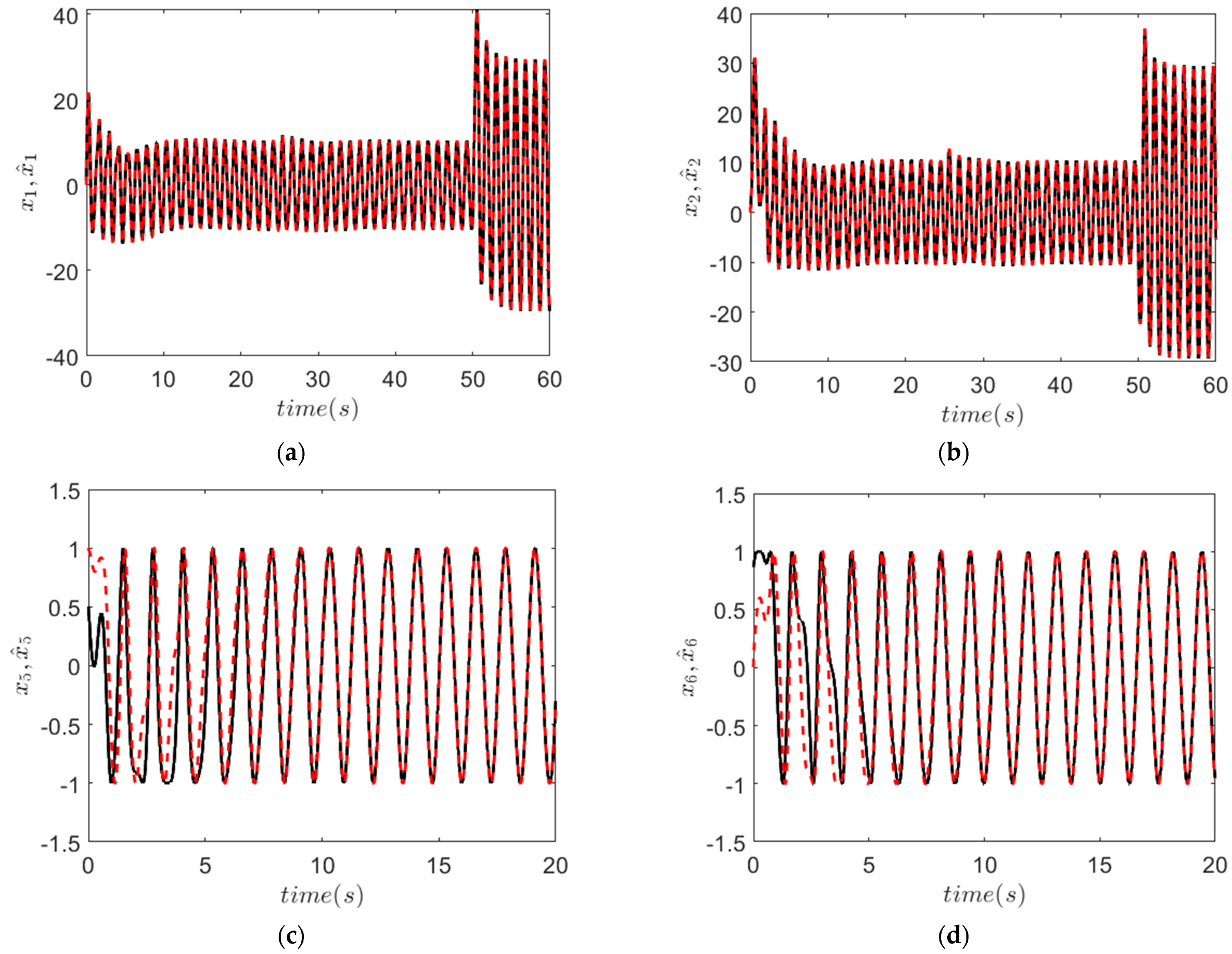
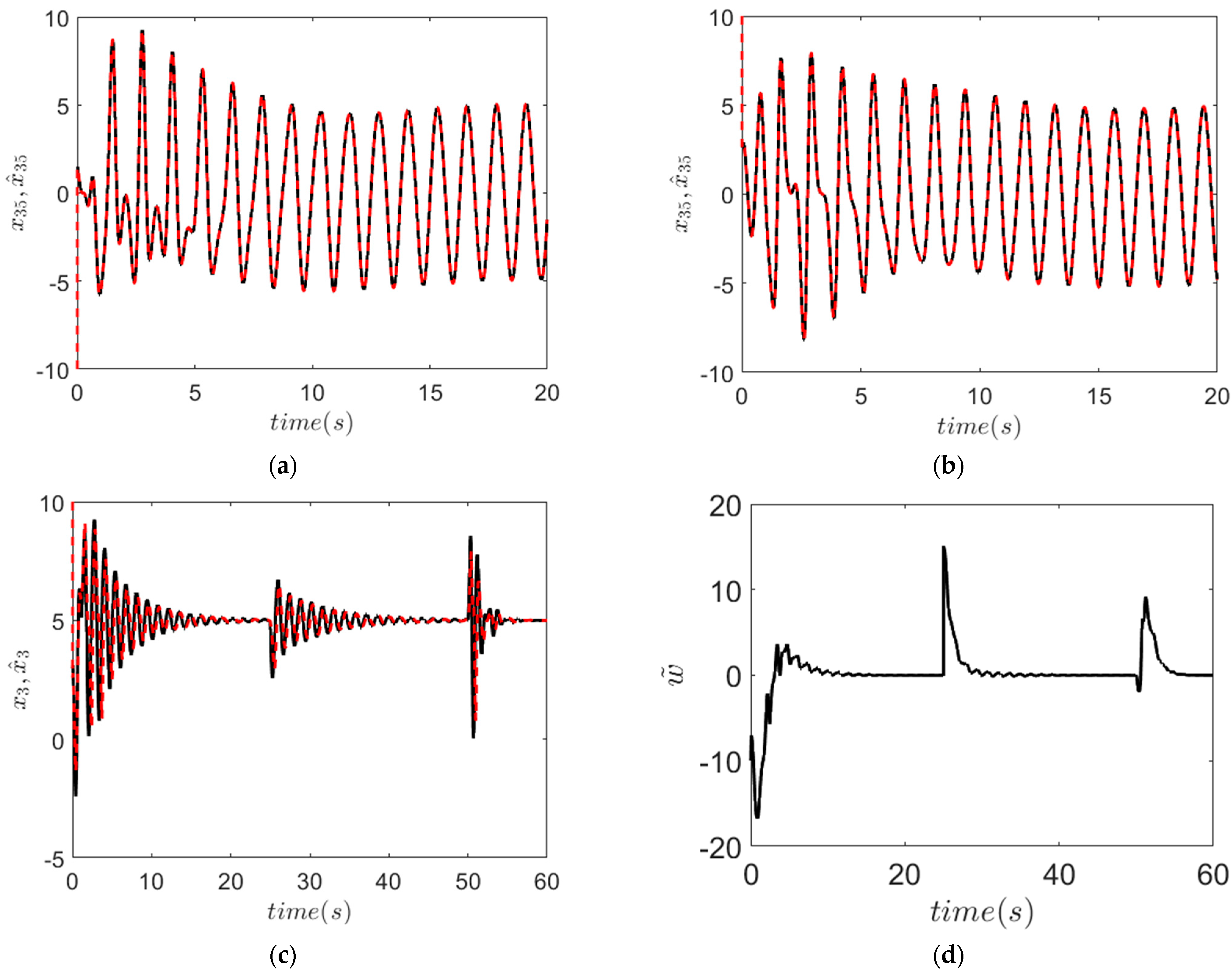
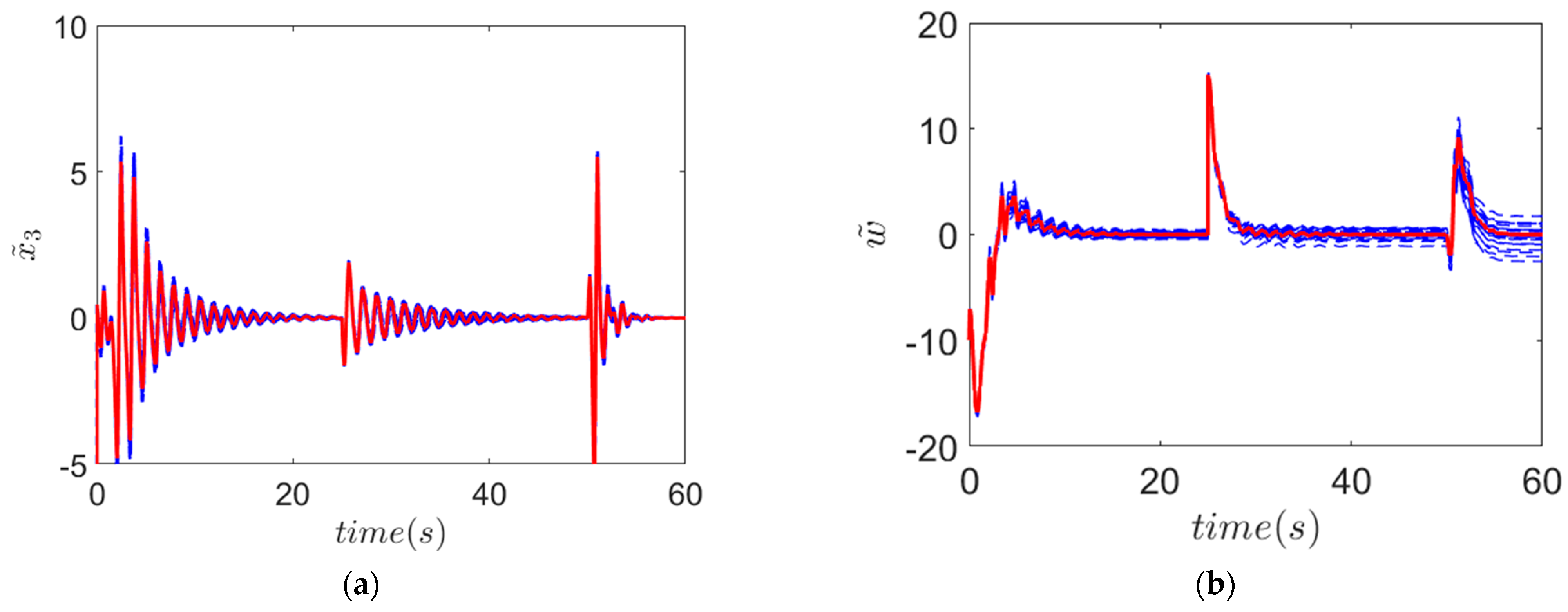
7. Numerical Simulations

For the PMSM model that is given in Section 2 and using the observer that is designed as detailed in Section 3, to analyze the performance of the nonlinear observer that is designed using numerical optimization tools YALMIP, MOSEK, and PENLAB, a set of numerical simulations are conducted using MATLAB [41,42,43]. The parameters of the PMSM model are given as $\left[p_1,p_2,p_3,p_4,p_5\right]=\left[-1,10,10,-1.5,-1\right]$. The speed estimator terms are given as

$$R_1\left({\widehat{x}}_1\right)=92.7+1.2{\left({\widehat{x}}_1\right)}^2$$

(53)

$$R_2\left({\widehat{x}}_2\right)=92.7+1.2{\left({\widehat{x}}_2\right)}^2$$

(54)

and the load-estimation-related terms are given as

$$R_{21}\left({\widehat{x}}_3,\widehat{w}\right)=1.16+0.53{\left({\widehat{x}}_3\right)}^2+0.53{\left(\widehat{w}\right)}^2$$

(55)

$$R_{22}\left({\widehat{x}}_3,\widehat{w}\right)=-8.7-1.2{\left({\widehat{x}}_3\right)}^2-1.2{\left(\widehat{w}\right)}^2$$

(56)

The resulting Lyapunov function for the estimation error dynamics is omitted due to space considerations. The simulation-related input and disturbance terms are given in

Table 1. Simulation input and disturbance terms during the operation.

Time (s)	Voltage Inputs	Load Term
0–25	$u_1=10\sin \left(2\pi \left[5\right]t\right)$ $u_2=10\sin \left(2\pi \left[5\right]t+\pi /2\right)$	$w=-10$
25–50	$u_1=10\sin \left(2\pi \left[5\right]t\right)$ $u_2=10\sin \left(2\pi \left[5\right]t+\pi /2\right)$	$w=5$
50–60	$u_1=20\sin \left(2\pi \left[5\right]t\right)$ $u_2=20\sin \left(2\pi \left[5\right]t+\pi /2\right)$	$w=5$

.

The state estimates that are produced by the first stage of the nonlinear observer are given in Figure 1, where the true $x_1,x_2$ states and $x_3,x_5$ states are estimated.

Using the $x_5,x_6$ estimates produced by the first stage of the nonlinear observer, $x_3$ and $w$ terms are estimated. In Figure 2, the estimation performance of $x_3{x}_5$ and $x_3{x}_6$ terms that are denoted by $x_{35}$ and $x_{36}$ are given. Using the $x_5$ and $x_6$ terms, the $x_3$ speed state is estimated, and it is given in Figure 2. Additionally, the load estimation error signal is given in Figure 2, which demonstrates the effect of load and input voltage fluctuations on the estimation and the capability of the observer to suppress the deteriorating effects of the changes.

In the second stage of the numerical simulations, the parameter uncertainty case is studied where parameters of the plant are perturbed, and the performance of the estimation algorithm, which is designed based on the nominal parameters given previously, is analyzed. As can be seen in Figure 3, the estimator is sufficient in dealing with the parameter uncertainty, where the parameters are perturbed up to 10% in the series of simulations. In general, the disturbance estimation is affected by the parameter uncertainty case, where the state estimation performance of the system stays unaffected.

8. Conclusions

In the paper, an SOS-optimization-based nonlinear observer design is studied. The final observer is designed to estimate the states and disturbance signals simultaneously. Considering a PMSM model, the design methodology is given in detail, and the performance of the observer is assessed using a numerical simulation. To reduce the general SOS optimization computation complexity and the problem dimension in general, exploiting the PMSM model structure, a cascaded nonlinear observer scheme is employed. In addition to that, since the measurements are a linear combination of the state vector, the general injection function is written as the function of the estimate terms, which also reduces the SOS optimization problem dimension. The given ISS problem formulation in terms of SOS optimization is another important step in formulating the general nonlinear observer design problem as an SOS feasibility problem which can be solved with the help of numerical optimization tools such as YALMIP, MOSEK, and PENLAB.

References

1. Park, I.; Kim, D.; Moon, J.; Kim, S.; Kang, Y.; Bae, S. Searching for New Technology Acceptance Model under Social Context: Analyzing the Determinants of Acceptance of Intelligent Information Technology in Digital Transformation and Implications for the Requisites of Digital Sustainability. Sustainability 2022, 14, 579. [Google Scholar] [CrossRef]
2. Wang, C.; Cao, D.; Qu, X.; Fan, C. An Improved Finite Control Set Model Predictive Current Control for a Two-Phase Hybrid Stepper Motor Fed by a Three-Phase VSI. Energies 2022, 15, 1222. [Google Scholar] [CrossRef]
3. Rasool, N.M.; Abbasoglu, S.; Hashemipour, M. Analysis and optimizes of hybrid wind and solar photovoltaic generation system for off-grid small village. J. Energy Syst. 2022, 6, 176–187. [Google Scholar] [CrossRef]
4. Thoppil, A.; Akbar, M.; Rambabu, D. Dynamic analysis of a tri-floater with vertical axis wind turbine supported at its centroid. J. Energy Syst. 2021, 5, 10–19. [Google Scholar] [CrossRef]
5. Lee, C.-Y.; Zhuo, G.-L.; Le, T.-A. A Robust Deep Neural Network for Rolling Element Fault Diagnosis under Various Operating and Noisy Conditions. Sensors 2022, 22, 4705. [Google Scholar] [CrossRef]
6. Liu, Y.; Fang, J.; Tan, K.; Huang, B.; He, W. Sliding Mode Observer with Adaptive Parameter Estimation for Sensorless Control of IPMSM. Energies 2020, 13, 5991. [Google Scholar] [CrossRef]
7. Kim, T.; Park, T.-H. Extended Kalman Filter (EKF) Design for Vehicle Position Tracking Using Reliability Function of Radar and Lidar. Sensors 2020, 20, 4126. [Google Scholar] [CrossRef]
8. Lv, M.; Li, X.; Li, Y.; Zhang, W.; Guo, R. UKF-Based State Estimation for Electrolytic Oxygen Generation System of Space Station. Appl. Sci. 2021, 11, 2021. [Google Scholar] [CrossRef]
9. Elfring, J.; Torta, E.; van de Molengraft, R. Particle Filters: A Hands-On Tutorial. Sensors 2021, 21, 438. [Google Scholar] [CrossRef]
10. Huang, Y.-S.; Sheriff, M.Z.; Bachawala, S.; Gonzalez, M.; Nagy, Z.K.; Reklaitis, G.V. Evaluation of a Combined MHE-NMPC Approach to Handle Plant-Model Mismatch in a Rotary Tablet Press. Processes 2021, 9, 1612. [Google Scholar] [CrossRef]
11. Aliskan, I. Adaptive Model Predictive Control for Wiener Nonlinear Systems. Iran. J. Sci. Technol. 2019, 43, 361–377. [Google Scholar] [CrossRef]
12. Sriram, C.; Somlal, J.; Goud, B.S.; Bajaj, M.; Elnaggar, M.F.; Kamel, S. Improved Deep Neural Network (IDNN) with SMO Algorithm for Enhancement of Third Zone Distance Relay under Power Swing Condition. Mathematics 2022, 10, 1944. [Google Scholar] [CrossRef]
13. Rodriguez-Mata, A.E.; Bustos-Terrones, Y.; Gonzalez-Huitrón, V.; Lopéz-Peréz, P.A.; Hernández-González, O.; Amabilis-Sosa, L.E. A Fractional High-Gain Nonlinear Observer Design—Application for Rivers Environmental Monitoring Model. Math. Comput. Appl. 2020, 25, 44. [Google Scholar] [CrossRef]
14. Butkus, M.; Levišauskas, D.; Galvanauskas, V. Simple Gain-Scheduled Control System for Dissolved Oxygen Control in Bioreactors. Processes 2021, 9, 1493. [Google Scholar] [CrossRef]
15. Jiao, Z.; Wu, J.; Chen, Z.; Wang, F.; Li, L.; Kong, Q.; Lin, F. Research on Takagi-Sugeno Fuzzy-Model-Based Vehicle Stability Control for Autonomous Vehicles. Actuators 2022, 11, 143. [Google Scholar] [CrossRef]
16. Lien, Y.-H.; Peng, C.-C.; Chen, Y.-H. Adaptive Observer-Based Fault Detection and Fault-Tolerant Control of Quadrotors under Rotor Failure Conditions. Appl. Sci. 2020, 10, 3503. [Google Scholar] [CrossRef]
17. Wang, Y.; Yu, H.; Che, Z.; Wang, Y.; Zeng, C. Extended State Observer-Based Predictive Speed Control for Permanent Magnet Linear Synchronous Motor. Processes 2019, 7, 618. [Google Scholar] [CrossRef]
18. Zhang, C.; Guo, C.; Zhang, D. Data Fusion Based on Adaptive Interacting Multiple Model for GPS/INS Integrated Navigation System. Appl. Sci. 2018, 8, 1682. [Google Scholar] [CrossRef]
19. Coelho, M.; Bousson, K.; Ahmed, K. An Improved Extended Kalman Filter for Radar Tracking of Satellite Trajectories. Designs 2021, 5, 54. [Google Scholar] [CrossRef]
20. Ran, C.; Cheng, X. A Direct and Non-Singular UKF Approach Using Euler Angle Kinematics for Integrated Navigation Systems. Sensors 2016, 16, 1415. [Google Scholar] [CrossRef] [Green Version]
21. Peng, C.-C. Nonlinear Integral Type Observer Design for State Estimation and Unknown Input Reconstruction. Appl. Sci. 2017, 7, 67. [Google Scholar] [CrossRef]
22. Charitopoulos, V.M.; Papageorgiou, L.G.; Dua, V. Multi Set-Point Explicit Model Predictive Control for Nonlinear Process Systems. Processes 2021, 9, 1156. [Google Scholar] [CrossRef]
23. Ali, I.A.; Elshafei, A.L. Model predictive control stabilization of a power system including a wind power plant. J. Energy Syst. 2022, 6, 188–208. [Google Scholar] [CrossRef]
24. Chan, J.C.L.; Lee, T.H. Sliding Mode Observer-Based Fault-Tolerant Secondary Control of Microgrids. Electronics 2020, 9, 1417. [Google Scholar] [CrossRef]
25. Wang, P.; Zhang, C.; Zhu, L.; Wang, C. High-Gain Observer-Based Sliding-Mode Dynamic Surface Control for Particleboard Glue Mixing and Dosing System. Algorithms 2018, 11, 166. [Google Scholar] [CrossRef]
26. Silva, S.N.; Lopes, F.F.; Valderrama, C.; Fernandes, M.A.C. Proposal of Takagi–Sugeno Fuzzy-PI Controller Hardware. Sensors 2020, 20, 1996. [Google Scholar] [CrossRef]
27. Ellouze, A.; Kahouli, O.; Ksantini, M.; Rebhi, A.; Hnaien, N.; Delmotte, F. Continuous Stability TS Fuzzy Systems Novel Frame Controlled by a Discrete Approach and Based on SOS Methodology. Mathematics 2021, 9, 3129. [Google Scholar] [CrossRef]
28. Ahmed, H.; Benbouzid, M. Adaptive Observer-Based Grid-Synchronization and Sequence Extraction Techniques for Renewable Energy Systems: A Comparative Analysis. Appl. Sci. 2021, 11, 653. [Google Scholar] [CrossRef]
29. He, F.; Cao, D.; Wu, J.; Li, J. Event-Triggered, Adaptive, Exponentially Asymptotic Tracking Control of Stochastic Nonlinear Systems. Symmetry 2022, 14, 451. [Google Scholar] [CrossRef]
30. Hoai, H.-K.; Chen, S.-C.; Than, H. Realization of the Sensorless Permanent Magnet Synchronous Motor Drive Control System with an Intelligent Controller. Electronics 2020, 9, 365. [Google Scholar] [CrossRef] [Green Version]
31. Furmanik, M.; Gorel, L.; Konvičný, D.; Rafajdus, P. Comparative Study and Overview of Field-Oriented Control Techniques for Six-Phase PMSMs. Appl. Sci. 2021, 11, 7841. [Google Scholar] [CrossRef]
32. Matthew, M.P. Full-State Feedback of Delayed Systems using SOS: A New Theory of Duality. IFAC Proc. Vol. 2013, 46, 24–29. [Google Scholar] [CrossRef]
33. Wang, T.-C.; Lall, S.; Chiou, T.-Y. Polynomial Method for PLL Controller Optimization. Sensors 2011, 11, 6575–6592. [Google Scholar] [CrossRef]
34. Alessandri, A. Lyapunov Functions for State Observers of Dynamic Systems Using Hamilton–Jacobi Inequalities. Mathematics 2020, 8, 202. [Google Scholar] [CrossRef]
35. Pitarch, J.L.; Sala, A.; de Prada, C. A Systematic Grey-Box Modeling Methodology via Data Reconciliation and SOS Constrained Regression. Processes 2019, 7, 170. [Google Scholar] [CrossRef]
36. Chiu, C.-H.; Peng, Y.-F. Design of Takagi-Sugeno Fuzzy Control Scheme for Real World System Control. Sustainability 2019, 11, 3855. [Google Scholar] [CrossRef]
37. Pylorof, D.; Bakolas, E.; Chan, K.S. Design of Robust Lyapunov-Based Observers for Nonlinear Systems with Sum-of-Squares Programming. IEEE Control Syst. Lett. 2020, 4, 283–288. [Google Scholar] [CrossRef]
38. Clarke, F.H.; Ledyaev, Y.S.; Sontag, E.D.; Subbotin, A.I. Asymptotic controllability implies feedback stabilization. IEEE Trans. Autom. Control 1997, 42, 1394–1407. [Google Scholar] [CrossRef]
39. Xue, Y.; Zhao, P. Input-to-State Stability and Stabilization of Nonlinear Impulsive Positive Systems. Mathematics 2021, 9, 1663. [Google Scholar] [CrossRef]
40. Ichihara, H. Sum of squares based input-to-state stability analysis of polynomial nonlinear systems. SICE J. Control. Meas. Syst. Integr. 2012, 5, 218–225. [Google Scholar] [CrossRef]
41. Löfberg, J. YALMIP: A toolbox for modeling and optimization in MATLAB. In Proceedings of the 2004 IEEE International Symposium on Computer Aided Control Systems Design, Taipei, Taiwan, 2–4 September 2004. [Google Scholar]
42. ApS, M. Mosek optimization toolbox for matlab. In User’s Guide and Reference Manual; Version 4; MOSEK: Copenhagen, Denmark, 2019. [Google Scholar]
43. Fiala, J.; Kocvara, M.; Stingl, M. PENLAB: A MATLAB solver for nonlinear semidefinite optimization. arXiv 2013, arXiv:1311.5240. [Google Scholar]
Figure 1. Estimation performances: black line for true signal, red line for estimated signal. (a) x 1 estimation, (b) x 2 estimation, (c) x 5 estimation, (d) x 5 estimation.
Sustainability 14 10650 g001
Figure 2. Estimation performances: black line for true signal, red line for estimated signal. (a) x 35 estimation, (b) x 36 estimation, (c) x 3 estimation, (d) w error signal.
Sustainability 14 10650 g002
Figure 3. Estimation performances: blue lines for perturbed parameters, red line for true parameters. (a) x 3 estimation, (b) w error signal.
Sustainability 14 10650 g003